EUROPEAN ORGANIZATION FOR NUCLEAR RESEARCH

CERN-EP/2001-052

3 July 2001

Angular Analysis of the Muon Pair Asymmetry at LEP 1

The OPAL Collaboration

Data on muon pair production obtained by the OPAL collaboration at centre of mass energies near the Z peak are analysed. Small angular mismatches between the directions of the two muons are used to assess the effects of initial state photon radiation and initial-final-state radiation interference on the forward-backward asymmetry of muon pairs. The dependence of the asymmetry on the invariant mass of the pair is measured in a model-independent way. Effective vector and axial-vector couplings of the Z boson are determined and compared to the Standard Model expectations.

To be published in Phys. Lett. B

G. Abbiendi², C. Ainsley⁵, P.F. Åkesson³, G. Alexander²², J. Allison¹⁶, G. Anagnostou¹, K.J. Anderson⁹, S. Arcelli¹⁷, S. Asai²³, D. Axen²⁷, G. Azuelos^18,a, I. Bailey²⁶, E. Barberio⁸, R.J. Barlow¹⁶, R.J. Batley⁵, T. Behnke²⁵, K.W. Bell²⁰, P.J. Bell¹, G. Bella²², A. Bellerive⁹, S. Bethke³², O. Biebel³², I.J. Bloodworth¹, O. Boeriu¹⁰, P. Bock¹¹, J. Böhme²⁵, D. Bonacorsi², M. Boutemeur³¹, S. Braibant⁸, L. Brigliadori², R.M. Brown²⁰, H.J. Burckhart⁸, J. Cammin³, R.K. Carnegie⁶, B. Caron²⁸, A.A. Carter¹³, J.R. Carter⁵, C.Y. Chang¹⁷, D.G. Charlton^1,b, P.E.L. Clarke¹⁵, E. Clay¹⁵, I. Cohen²², J. Couchman¹⁵, A. Csilling^8,i, M. Cuffiani², S. Dado²¹, G.M. Dallavalle², S. Dallison¹⁶, A. De Roeck⁸, E.A. De Wolf⁸, P. Dervan¹⁵, K. Desch²⁵, B. Dienes³⁰, M.S. Dixit^6,a, M. Donkers⁶, J. Dubbert³¹, E. Duchovni²⁴, G. Duckeck³¹, I.P. Duerdoth¹⁶, E. Etzion²², F. Fabbri², L. Feld¹⁰, P. Ferrari¹², F. Fiedler⁸, I. Fleck¹⁰, M. Ford⁵, A. Frey⁸, A. Fürtjes⁸, D.I. Futyan¹⁶, P. Gagnon¹², J.W. Gary⁴, G. Gaycken²⁵, C. Geich-Gimbel³, G. Giacomelli², P. Giacomelli², D. Glenzinski⁹, J. Goldberg²¹, K. Graham²⁶, E. Gross²⁴, J. Grunhaus²², M. Gruwé⁸, P.O. Günther³, A. Gupta⁹, C. Hajdu²⁹, M. Hamann²⁵, G.G. Hanson¹², K. Harder²⁵, A. Harel²¹, M. Harin-Dirac⁴, M. Hauschild⁸, J. Hauschildt²⁵, C.M. Hawkes¹, R. Hawkings⁸, R.J. Hemingway⁶, C. Hensel²⁵, G. Herten¹⁰, R.D. Heuer²⁵, J.C. Hill⁵, K. Hoffman⁹, R.J. Homer¹, D. Horváth^29,c, K.R. Hossain²⁸, R. Howard²⁷, P. Hüntemeyer²⁵, P. Igo-Kemenes¹¹, K. Ishii²³, A. Jawahery¹⁷, H. Jeremie¹⁸, C.R. Jones⁵, P. Jovanovic¹, T.R. Junk⁶, N. Kanaya²⁶, J. Kanzaki²³, G. Karapetian¹⁸, D. Karlen⁶, V. Kartvelishvili¹⁶, K. Kawagoe²³, T. Kawamoto²³, R.K. Keeler²⁶, R.G. Kellogg¹⁷, B.W. Kennedy²⁰, D.H. Kim¹⁹, K. Klein¹¹, A. Klier²⁴, S. Kluth³², T. Kobayashi²³, M. Kobel³, T.P. Kokott³, S. Komamiya²³, R.V. Kowalewski²⁶, T. Krämer²⁵, T. Kress⁴, P. Krieger⁶, J. von Krogh¹¹, D. Krop¹², T. Kuhl³, M. Kupper²⁴, P. Kyberd¹³, G.D. Lafferty¹⁶, H. Landsman²¹, D. Lanske¹⁴, I. Lawson²⁶, J.G. Layter⁴, A. Leins³¹, D. Lellouch²⁴, J. Letts¹², L. Levinson²⁴, J. Lillich¹⁰, C. Littlewood⁵, S.L. Lloyd¹³, F.K. Loebinger¹⁶, G.D. Long²⁶, M.J. Losty^6,a, J. Lu²⁷, J. Ludwig¹⁰, A. Macchiolo¹⁸, A. Macpherson^28,l, W. Mader³, S. Marcellini², T.E. Marchant¹⁶, A.J. Martin¹³, J.P. Martin¹⁸, G. Martinez¹⁷, G. Masetti², T. Mashimo²³, P. Mättig²⁴, W.J. McDonald²⁸, J. McKenna²⁷, T.J. McMahon¹, R.A. McPherson²⁶, F. Meijers⁸, P. Mendez-Lorenzo³¹, W. Menges²⁵, F.S. Merritt⁹, H. Mes^6,a, A. Michelini², S. Mihara²³, G. Mikenberg²⁴, D.J. Miller¹⁵, S. Moed²¹, W. Mohr¹⁰, T. Mori²³, A. Mutter¹⁰, K. Nagai¹³, I. Nakamura²³, H.A. Neal³³, R. Nisius⁸, S.W. O’Neale¹, A. Oh⁸, A. Okpara¹¹, M.J. Oreglia⁹, S. Orito²³, C. Pahl³², G. Pásztor^8,i, J.R. Pater¹⁶, G.N. Patrick²⁰, J.E. Pilcher⁹, J. Pinfold²⁸, D.E. Plane⁸, B. Poli², J. Polok⁸, O. Pooth⁸, A. Quadt³, K. Rabbertz⁸, C. Rembser⁸, P. Renkel²⁴, H. Rick⁴, N. Rodning²⁸, J.M. Roney²⁶, S. Rosati³, K. Roscoe¹⁶, Y. Rozen²¹, K. Runge¹⁰, D.R. Rust¹², K. Sachs⁶, T. Saeki²³, O. Sahr³¹, E.K.G. Sarkisyan^8,m, C. Sbarra²⁶, A.D. Schaile³¹, O. Schaile³¹, P. Scharff-Hansen⁸, M. Schröder⁸, M. Schumacher²⁵, C. Schwick⁸, W.G. Scott²⁰, R. Seuster^14,g, T.G. Shears^8,j, B.C. Shen⁴, C.H. Shepherd-Themistocleous⁵, P. Sherwood¹⁵, A. Skuja¹⁷, A.M. Smith⁸, G.A. Snow¹⁷, R. Sobie²⁶, S. Söldner-Rembold^10,e, S. Spagnolo²⁰, F. Spano⁹, M. Sproston²⁰, A. Stahl³, K. Stephens¹⁶, D. Strom¹⁹, R. Ströhmer³¹, L. Stumpf²⁶, B. Surrow²⁵, S. Tarem²¹, M. Tasevsky⁸, R.J. Taylor¹⁵, R. Teuscher⁹, J. Thomas¹⁵, M.A. Thomson⁵, E. Torrence¹⁹, D. Toya²³, T. Trefzger³¹, A. Tricoli², I. Trigger⁸, Z. Trócsányi^30,f, E. Tsur²², M.F. Turner-Watson¹, I. Ueda²³, B. Ujvári^30,f, B. Vachon²⁶, C.F. Vollmer³¹, P. Vannerem¹⁰, M. Verzocchi¹⁷, H. Voss⁸, J. Vossebeld⁸, D. Waller⁶, C.P. Ward⁵, D.R. Ward⁵, P.M. Watkins¹, A.T. Watson¹, N.K. Watson¹, P.S. Wells⁸, T. Wengler⁸, N. Wermes³, D. Wetterling¹¹ G.W. Wilson¹⁶, J.A. Wilson¹, T.R. Wyatt¹⁶, S. Yamashita²³, V. Zacek¹⁸, D. Zer-Zion^8,k

¹School of Physics and Astronomy, University of Birmingham, Birmingham B15 2TT, UK
²Dipartimento di Fisica dell’ Università di Bologna and INFN, I-40126 Bologna, Italy
³Physikalisches Institut, Universität Bonn, D-53115 Bonn, Germany
⁴Department of Physics, University of California, Riverside CA 92521, USA
⁵Cavendish Laboratory, Cambridge CB3 0HE, UK
⁶Ottawa-Carleton Institute for Physics, Department of Physics, Carleton University, Ottawa, Ontario K1S 5B6, Canada
⁸CERN, European Organisation for Nuclear Research, CH-1211 Geneva 23, Switzerland
⁹Enrico Fermi Institute and Department of Physics, University of Chicago, Chicago IL 60637, USA
¹⁰Fakultät für Physik, Albert Ludwigs Universität, D-79104 Freiburg, Germany
¹¹Physikalisches Institut, Universität Heidelberg, D-69120 Heidelberg, Germany
¹²Indiana University, Department of Physics, Swain Hall West 117, Bloomington IN 47405, USA
¹³Queen Mary and Westfield College, University of London, London E1 4NS, UK
¹⁴Technische Hochschule Aachen, III Physikalisches Institut, Sommerfeldstrasse 26-28, D-52056 Aachen, Germany
¹⁵University College London, London WC1E 6BT, UK
¹⁶Department of Physics, Schuster Laboratory, The University, Manchester M13 9PL, UK
¹⁷Department of Physics, University of Maryland, College Park, MD 20742, USA
¹⁸Laboratoire de Physique Nucléaire, Université de Montréal, Montréal, Quebec H3C 3J7, Canada
¹⁹University of Oregon, Department of Physics, Eugene OR 97403, USA
²⁰CLRC Rutherford Appleton Laboratory, Chilton, Didcot, Oxfordshire OX11 0QX, UK
²¹Department of Physics, Technion-Israel Institute of Technology, Haifa 32000, Israel
²²Department of Physics and Astronomy, Tel Aviv University, Tel Aviv 69978, Israel
²³International Centre for Elementary Particle Physics and Department of Physics, University of Tokyo, Tokyo 113-0033, and Kobe University, Kobe 657-8501, Japan
²⁴Particle Physics Department, Weizmann Institute of Science, Rehovot 76100, Israel
²⁵Universität Hamburg/DESY, II Institut für Experimental Physik, Notkestrasse 85, D-22607 Hamburg, Germany
²⁶University of Victoria, Department of Physics, P O Box 3055, Victoria BC V8W 3P6, Canada
²⁷University of British Columbia, Department of Physics, Vancouver BC V6T 1Z1, Canada
²⁸University of Alberta, Department of Physics, Edmonton AB T6G 2J1, Canada
²⁹Research Institute for Particle and Nuclear Physics, H-1525 Budapest, P O Box 49, Hungary
³⁰Institute of Nuclear Research, H-4001 Debrecen, P O Box 51, Hungary
³¹Ludwigs-Maximilians-Universität München, Sektion Physik, Am Coulombwall 1, D-85748 Garching, Germany
³²Max-Planck-Institute für Physik, Föhring Ring 6, 80805 München, Germany
³³Yale University,Department of Physics,New Haven, CT 06520, USA

^a and at TRIUMF, Vancouver, Canada V6T 2A3
^b and Royal Society University Research Fellow
^c and Institute of Nuclear Research, Debrecen, Hungary
^e and Heisenberg Fellow
^f and Department of Experimental Physics, Lajos Kossuth University, Debrecen, Hungary
^g and MPI München
ⁱ and Research Institute for Particle and Nuclear Physics, Budapest, Hungary
^j now at University of Liverpool, Dept of Physics, Liverpool L69 3BX, UK
^k and University of California, Riverside, High Energy Physics Group, CA 92521, USA
^l and CERN, EP Div, 1211 Geneva 23
^m and Tel Aviv University, School of Physics and Astronomy, Tel Aviv 69978, Israel.

1 Introduction

Many experiments have studied the forward-backward asymmetry of muon pairs produced in electron positron annihilation [1, 2, 3], motivated by its sensitivity to interference between the axial-vector coupling of the ${\mathrm{Z}}$ and the vector couplings of the ${\mathrm{Z}}$ and the photon, the clean signature of the muons, and the lack of complications from $t$-channel exchange. The asymmetry depends on the centre of mass energy and, at tree level near the ${\mathrm{Z}}$ peak, this dependence is described by a straight line [4], with a slope and intercept directly related to parameters of the Z boson.

In the conventional method of analysis, however, the asymmetry is measured within a kinematic phase-space which integrates over the spectrum of radiated photons. This integrated asymmetry is then compared with the predictions of a theoretical model, whose parameters are varied to produce the optimum agreement. The integration over the spectrum of radiated photons noticeably changes the energy dependence of the asymmetry through two effects:

• Initial State Radiation (ISR) lowers the effective centre of mass energy of the event, so the muon pair has an angular distribution which is appropriate to a lower energy and, furthermore, is distorted by the Lorentz boost.

• Interference between photons emitted in the initial and final state (IFI) distorts the angular distribution from the usual $1+\cos^{2}\theta+a\cos\theta$ dependence and produces a forward-backward asymmetry, strongly dependent on angular cuts, even in the absence of any axial coupling [5].

These effects depend on the centre of mass (CM) energy (e.g., the intensity of ISR increases strongly when the energy exceeds the ${\mathrm{Z}}$ mass) and significantly distort the asymmetry at the levels of precision obtained by the LEP 1 experiments [2, 3].

In conventional analyses ISR is modelled by folding a radiator function calculated in QED with a Breit-Wigner model of the resonance cross section. For the effects of IFI, conventional analyses rely on the large cancellation expected if the cuts are set wide, i.e. when the cross section is integrated over a phase space which accepts almost all radiation from the initial and final states and the interference between the two[6]. This integration represents a loss of angular information and the cancellation has not previously been verified experimentally.

We present here an analysis which explicitly studies the effects of electromagnetic radiative corrections for muon pairs:

• We consider ISR on an event-by-event basis. This enables us to assess the effective invariant mass of the muon pair, and thus study the variation of the asymmetry with energy, even at a single energy of the colliding beams.

• We measure the effect of IFI on the angular distributions. By analysing small angular mismatches between the directions of the two muons it is possible to identify and study those areas of the phase space where the IFI-induced asymmetry is significant, and see how the above-mentioned cancellation works.

Our approach enables us to measure the Z boson effective couplings in a model-independent way, using only asymmetry measurements around the Z peak. The only assumptions used are those of QED, electron-muon universality, and the spin-1 nature of the Z boson. Our analysis is based on the measured properties of the $\mu^{+}\mu^{-}$ pair alone, and does not directly involve the detection of the radiated photons, which often escape direct detection either because of their low energy or because they go down the beam pipe. It thus includes the effect of soft radiative corrections, in contrast to approaches utilizing detected photons, which probe only hard corrections [7].

2 Choice of variables

At tree level, muon pair production in $\mbox{e}^{+}\mbox{e}^{-}$-annihilation is a straightforward $2\to 2$ process:

$${}\mathrm{e^{+}e^{-}}\to\mu^{+}\mu^{-}$$ (1)

with the two final-state muons exactly back-to-back in the centre of mass (CM) system. For unpolarised beams, the azimuthal orientation of the event does not carry any useful information, and there is only one angle of interest, which can be chosen to be the polar angle of either of the two final-state muons $\theta^{\pm}$. Here we adopt the usual coordinate conventions, where the electron beam direction is along the $+z$ axis of a right-handed cartesian system. The polar angles of the outgoing $\mu^{-}$ and $\mu^{+}$ with respect to this direction are respectively $\theta^{-}$ and $\theta^{+}$, and the corresponding azimuthal angles $\phi^{-}$ and $\phi^{+}$ are measured with respect to the $x$-axis, which points to the centre of the LEP ring.

Higher-order corrections give rise to the radiation of real photons:

$${}\mathrm{e^{+}e^{-}}\to\mu^{+}\mu^{-}\gamma(\gamma\dots)$$ (2)

The radiated photons are not always directly observable: they may have very low energy, or may be radiated along the beam pipe, thus missing the detector altogether. But the photons can still be accounted for by measuring the angular mismatch between the directions of the muons. Since the two muons are no longer back-to-back, one needs three non-trivial angular variables to describe their directions. An especially convenient set is $\theta^{\bullet}$, $\eta$ and $\xi$.

Following [8] the angle $\theta^{\bullet}$ is defined by:

$${}\cos\theta^{\bullet}={{\sin(\theta^{-}-\theta^{+})}\over{\sin\theta^{-}+\sin\theta^{+}}}.$$ (3)

It reduces to $\cos\theta^{\bullet}=\cos\theta^{+}=-\cos\theta^{-}$ when $\theta^{+}=\pi-\theta^{-}$. In the case of ISR collinear with the beam direction, $\cos\theta^{\bullet}$ equals $\cos\theta^{+}$ in the CM system of the muon pair.

The variable $\eta$ also depends only on $\theta^{+}$ and $\theta^{-}$:

$$\eta = {{|\sin(\theta^{+}+\theta^{-})|}\over{|\sin(\theta^{+}+\theta^{-})|+\sin\theta^{+}+\sin\theta^{-}}}{}.$$ (4)

If a photon is radiated exactly along the beam direction, $\eta$ is the boost parameter and the energy of the photon, $E_{\gamma}$, is

$$E_{\gamma} = \eta\;\sqrt{s}.$$ (5)

In this case, $\eta$ measures the mismatch between the polar angles of the two muons, and is equal to zero if the muons are back-to-back. The invariant mass squared $s^{\prime}$ of the muon pair is then given by

$${}s^{\prime}=(1-2\eta)s.$$ (6)

The acoplanarity $\xi$ is defined in the $x-y$ plane:

$${}\xi={\Bigl{|}}{\left|\phi^{+}-\phi^{-}\right|}-\pi{\Bigr{|}}.$$ (7)

It measures the angular mismatch between the two muons in the transverse direction, and is also equal to zero if the muons are back-to-back.

Conventional analyses often use the acollinearity angle $\zeta$  defined through the 3-momenta $\vec{p}_{\pm}$ of the final muons:

$${}\cos\zeta=-{{\vec{p}_{+}\cdot\vec{p}_{-}}\over{|{\vec{p}_{+}||\vec{p}_{-}|}}}.$$ (8)

It combines the angular mismatch in $\theta$ with the mismatch in $\phi$. This is not sensible in experiments where the resolution of the $\phi$ measurement is significantly better than that of $\theta$. Moreover, a mismatch in $\theta$ is mostly due to strong ISR with the photon going along the beam direction, while a strong mismatch in $\phi$ is mostly due to photon radiation from one of the final state muons (FSR). These two processes, and their interference (IFI), have significantly different angular dependences, and their separation is an essential part of the present analysis. For these reasons, the acollinearity angle $\zeta$ is not used here.

3 Theoretical treatment

3.1 Tree level formulae

Consider first the (unphysical) case with no radiated photons, to which corrections will then be calculated. The normalised angular dependence of muon pair production at a CM energy $\sqrt{s}$ is given by:

$${}{{1}\over{\sigma(s)}}\;{{d^{3}\sigma(s)}\over{d\cos\theta\;d\xi\;d\eta}}=\Bigl{\{}\;{3\over 8}\;(1+\cos^{2}\theta)+A_{FB}(s)\;\cos\theta\Bigr{\}}\;\delta(\xi)\;\delta(\eta)$$ (9)

which has a trivial dependence on $\xi$ and $\eta$, described by the two Dirac $\delta$-functions. The coefficient $A_{FB}(s)$ of the term linear in $\cos\theta$ is the forward-backward asymmetry:

$$A_{FB}(s) = {{\sigma(\cos\theta>0)-\sigma(\cos\theta<0)}\over{\sigma(\cos\theta>0)+\sigma(\cos\theta<0)}}$$ (10)

$$= {{3}\over{4}}{{F_{3}(s)}\over{F_{1}(s)}}.$$ (11)

Assuming only that the Z boson is a massive spin-1 resonance with mass $M_{Z}$ and width $\Gamma_{Z}$, and following the notation of [3], the energy-dependent functions $F_{1,3}(s)$ near the ${\mathrm{Z}}$ peak have the following form [3, 9]:

$$F_{1}(s) = 1+2\;{\mathrm{Re}}\{\chi_{0}^{*}(s)\;C^{s}_{\gamma Z}\}+|\chi_{0}(s)|^{2}\;C^{s}_{ZZ},$$ (12)

$$F_{3}(s) = \;\;2\;{\mathrm{Re}}\{\chi_{0}^{*}(s)\;C^{a}_{\gamma Z}\}+4\;|\chi_{0}(s)|^{2}\;C^{a}_{ZZ},$$ (13)

where

$$\chi_{0}(s) = {{1}\over{K}}\;{{s}\over{s-M_{Z}^{2}+iM_{Z}\Gamma_{Z}}}{}.$$ (14)

Assuming electron-muon universality in vector and axial-vector couplings, $g^{e}_{V,A}=g^{\mu}_{V,A}\equiv g_{V,A}$, the coefficients $C$ take the form:

$$C^{s}_{\gamma Z}=g_{V}^{2} C^{s}_{ZZ}=(g_{V}^{2}+g_{A}^{2})^{2}\;,$$ , (15)

$$C^{a}_{\gamma Z}=g_{A}^{2} C^{a}_{ZZ}=g_{V}^{2}g_{A}^{2}\;.$$ , (16)

In the immediate vicinity of the ${\mathrm{Z}}$ pole the asymmetry (11) is a linear function of $s$:

$$A_{FB}(s) = \;\;\;\;\;\;{{3C^{a}_{ZZ}}\over{C^{s}_{ZZ}}}\;\;\;\;+\;\;{{s-M_{Z}^{2}}\over{2s}}\;K\;{{3C^{a}_{\gamma Z}}\over{C^{s}_{ZZ}}}$$ (17)

$$= {{3g_{V}^{2}g_{A}^{2}}\over{(g_{V}^{2}+g_{A}^{2})^{2}}}\;\;+\;\;{{{s}-M_{Z}^{2}}\over{2s}}\;K\;{{3g_{A}^{2}}\over{(g_{V}^{2}+g_{A}^{2})^{2}}}.$$ (18)

The first (constant) term in both (17) and (18), the asymmetry at peak, depends only on the ratio $g_{V}/g_{A}$, while the slope with energy of the second term allows one to measure the axial-vector leptonic coupling, $g_{A}$. The constant $K$, which stands for the ratio of the ${\mathrm{Z}}$ boson and photon propagator normalisation factors, determines the scale of the $g_{V}$ and $g_{A}$ parameters: only two of the three quantities $g_{V}$, $g_{A}$ and $K$ are independent, if asymmetry is the only measured quantity.

Note that eqs. (17) and (18) do not contain $\Gamma_{Z}$. In particular, the slope of the asymmetry with energy is independent of $\Gamma_{Z}$. The linear approximation remains valid over the region where the Z dominates the photon.

In the Standard Model, the constant $K$ is expressed through the ratio of the electromagnetic coupling $\alpha$ and the Fermi constant $G_{F}$:

$$K \equiv {{2\sqrt{2}\pi\alpha}\over{G_{F}M_{Z}^{2}}}{}$$ (19)

After the imaginary part of the photon propagator is taken into account, which results in a small offset in the forward-backward asymmetry at peak [12], eqs. (12—19) still hold [10, 11, 12] in what is called the “Improved Born Approximation”, with $g_{V}$ and $g_{A}$ now standing for the real parts of the effective vector and axial-vector couplings of the Z boson. The contributions of the imaginary remnants of the effective couplings are small, and have been neglected in this analysis. The numerical value of the normalisation constant $K$ changes as the scale dependence of the electromagnetic coupling is taken into account:

$$\alpha\to\alpha(M^{2}_{Z})\approx 1/128.89.$$ (20)

3.2 Radiative QED corrections

Initial state radiation (ISR), final state radiation (FSR) and the interference of the two (IFI) affect the angular distribution of final muons in different ways.

ISR photons are radiated mainly along the beam axis, and the CM frame of the muon pair acquires a boost. As mentioned above, under collinear ISR $\theta^{\bullet}$ remains equal to $\theta^{+}$ in this frame. The acoplanarity variable $\xi$, defined in the transverse plane, is also largely insensitive to ISR. The parameter $\eta$  however, is essentially proportional to the energy of the emitted photon. Thus, events with significant ISR typically have $\eta$ significantly larger than $\xi$. The angular distribution

$${}{{d^{2}\sigma}\over{d\cos\theta^{\bullet}\;d\eta}}\sim\Bigl{\{}\;{3\over 8}\;(1+\cos^{2}\theta^{\bullet})+{A_{FB}(s^{\prime})}\;\cos\theta^{\bullet}\Bigr{\}}\,f(\eta)$$ (21)

acquires a non-trivial $\eta$-dependence described by the function $f(\eta)$, and an additional $\eta$-dependence through the argument $s^{\prime}=(1-2\eta)s$ of the asymmetric term $A_{FB}(s^{\prime})$. So, the measurement of the mismatch in the polar angles of the two muons, described by the variable $\eta$, allows the forward-backward asymmetry $A_{FB}$ to be measured directly at various energies $\sqrt{s^{\prime}}$, below and up to the actual initial CM energy, $\sqrt{s}$.

FSR is essentially symmetric around the final muon direction, and an angular mismatch in the longitudinal direction is close to that in the transverse direction, yielding on average $\eta\simeq\xi$. FSR is mainly directed along the final muons, and its effect alone on the forward-backward asymmetry is unmeasurably small.

Radiation with significant initial-final interference, IFI, is concentrated also mainly in the areas where $\eta\simeq\xi$. It is a complicated function of all three angular variables and contains a term which is odd in $\cos\theta^{\bullet}$, thus introducing an additional forward-backward asymmetry. This is expected to be positive for softer photons, $E_{\gamma}\lesssim\Gamma_{Z}/2$, and negative for harder ones. This strong variation of the asymmetry as a function of acoplanarity has been observed in [13]. For a totally inclusive treatment (when one integrates over all values of $\eta$ and $\xi$), IFI should have a negligible effect on the asymmetry, as these two regions cancel each other almost completely [6]. By measuring $\eta$ and $\xi$ we can identify those areas of the phase space where this IFI-induced asymmetry is significant and check the mechanics of the expected cancellation.

Consider a tight cut on acoplanarity $\xi<\xi_{0}$. This restricts the phase space of the radiated photon and disturbs the delicate balance required for the cancellation of the initial-final interference effects. The additional asymmetric term, which enters the expression for the full differential cross section, has a characteristic logarithmic dependence on $\cos\theta^{\bullet}$ [12, 14]:

$$\int^{\xi_{0}}_{0}d\xi\;{{d^{3}\sigma(s^{\prime})}\over{d\cos\theta^{\bullet}\;d\xi\;d\eta}}\sim\Bigl{\{}\;{3\over 8}\;(1+\cos^{2}\theta^{\bullet})+A_{FB}((1-2\eta)s)\;\cos\theta^{\bullet}\Bigr{\}}$$

$$\times\Bigl{\{}f_{+}(\eta)[1+\beta(\eta,\cos\theta^{\bullet})]+f_{-}(\eta){{1}\over{2}}\ln{{1+\cos\theta^{\bullet}}\over{1-\cos\theta^{\bullet}}}\Bigr{\}}.{}$$ (22)

The functions $\beta(\eta,\cos\theta^{\bullet})$ and $f_{\pm}(\eta)$ implicitly depend upon the value of the acoplanarity cut $\xi_{0}$; a complete theoretical calculation of these functions for arbitrary values of the cut $\xi_{0}$ would involve a detailed analysis of the participating interfering diagrams and the complete set of the SM parameters. However, the treatment is significantly simplified if the cut $\xi_{0}$ is chosen to be very tight, of order $10^{-3}$. In this case, the functions $f_{\pm}$ and $\beta$ can be calculated by numerical integration of the analytic formulae describing QED radiative corrections in the single soft photon approximation [14]. By comparing theoretical formulae and generator-level Monte Carlo simulations with [16, 15] and without [14, 17] exponentiation of radiative corrections, it was verified that the above approximation is adequate at energies around the ${\mathrm{Z}}$ peak, if $\xi$ and $\eta$ are small enough and one does not get too close to the edges of $\cos\theta^{\bullet}$ distribution.

In this approximation, the term with the function $f_{+}(\eta)$ contains the contributions from ISR, which is $\cos\theta^{\bullet}$-independent, and from the remnants of FSR, which result in an even $\cos\theta^{\bullet}$-dependence, described by the function $\beta(\eta,\cos\theta^{\bullet})$. The latter can be parametrised as

$$\beta(\eta,\cos\theta^{\bullet})={{f_{-}(\eta)}\over{f_{+}(\eta)}}{{1}\over{4\cos\theta^{\bullet}}}\ln{{1+\cos\theta^{\bullet}}\over{1-\cos\theta^{\bullet}}}$$ (23)

and, in the range of the angular variables considered in this analysis, represents a small ($\sim$ few percent) correction to the main symmetric term.

The last term in (22), with the function $f_{-}(\eta)$, describes the contribution of initial-final radiation interference, and has an odd $\cos\theta^{\bullet}$-dependence. This term is responsible for the additional asymmetry which arises because of the tight acoplanarity cut. Fortunately, the $\cos\theta^{\bullet}$-dependences of the two odd terms in (22) are significantly different, and, given the statistical power of the LEP 1 data set, these two asymmetric contributions can be separated.

4 Monte Carlo samples

Three Monte Carlo samples have been used at various stages of this study. They were obtained using KORALZ generator version 4.0 [17] and full OPAL detector simulation [18]. It is an important feature of this analysis that the numerical results obtained in Section 7 are, in fact, almost independent of these simulations, the samples being used only to assess systematic errors and derive a few small corrections.

The first sample contains 600000 muon pair events with soft photon exponentiation, but without the initial-final radiation interference. This sample, labelled “MC1”, was used to study resolutions and efficiencies, as described in subsections 5.2 and 7.1.

The second sample, labelled as “MC2”, contains 100000 events with the complete set of ${\cal O}(\alpha)$ corrections, which includes the initial-final radiation interference. Alongside with MC1, MC2 is used in Section 6 to illustrate the differences in the angular distributions of the various data subsamples.

The third sample contains 600000 $\tau$ pair events. It is referred to as “MC3”, and is used for background studies together with MC1, as described in the following section.

5 Event selection

Events collected by the OPAL experiment at LEP 1, at and around the ${\mathrm{Z}}$ peak during 1993, 1994 and 1995 are used in this study. The data correspond to total integrated luminosities of about 82 pb^-1 at the CM energy around 91.22 GeV (hereafter referred to as “peak”), 17 pb^-1 at 89.44 GeV (“peak$-$2”) and 18 pb^-1 at 92.97 GeV (“peak+2”).

A detailed description of the OPAL detector is given elsewhere [19, 20]. Here we briefly describe some subdetectors relevant to our analysis. Most of these form a set of coaxial cylinders, with varying coverage in $\theta$. The innermost is the central vertex detector, which consists of a set of axial (CVA) and stereo (CVS) wires, both with angular coverage $|\cos\theta|=0.92$. This is followed by the multi-wire jet chamber (CJ), which is surrounded by thin $z$-chambers (CZ), the latter covering the angular range $|\cos\theta|<0.72$. The coaxial magnetic field of 0.435 T allows the measurement of the momenta of charged particles. The following layer is formed by the electromagnetic (ECAL) and hadronic (HCAL) calorimeters. The outer layer consists of a set of barrel (MB) and endcap (ME) muon chambers.

5.1 Selection of Muon Pair Events and Background Rejection

Muons are identified either by hits in muon chambers (MB and/or ME) or by the specific pattern of energy deposition in HCAL or ECAL. Events passing the multihadron and cosmic veto and containing 2 tracks identified as muons are selected if the visible energy in the event (defined as the sum of the two muon energies and the highest energy ECAL cluster in the event) is larger than $0.6\sqrt{s}$ (see [3] for details). This part of the $\mathrm{e}^{+}\mathrm{e}^{-}\to\mu^{+}\mu^{-}$ selection is identical to that described in [3], except that here we do not require the cut on the acollinearity angle (8), but do require that the two muon tracks be measured to have opposite charges.

The visible energy cut is designed to reduce the only significant background to the processes (1,2), $\tau$ pair production, studied using Monte Carlo samples MC1 and MC3. In the usual inclusive asymmetry analysis this cut removes most of the $\tau\tau$ background, reducing its fraction in the data event sample to about 1%. However, $\tau\tau$ events have a much broader $\eta$-distribution than $\mu\mu$ events, and even this small amount of background can interfere with the analysis presented here. An additional cut is applied to the missing transverse momentum in the event:

$${}x_{T}=\sqrt{{\bigl{(}\Sigma p_{x}\bigr{)}^{2}+\bigl{(}\Sigma p_{y}\bigr{)}^{2}}\over{s}}\leq 0.1,$$ (24)

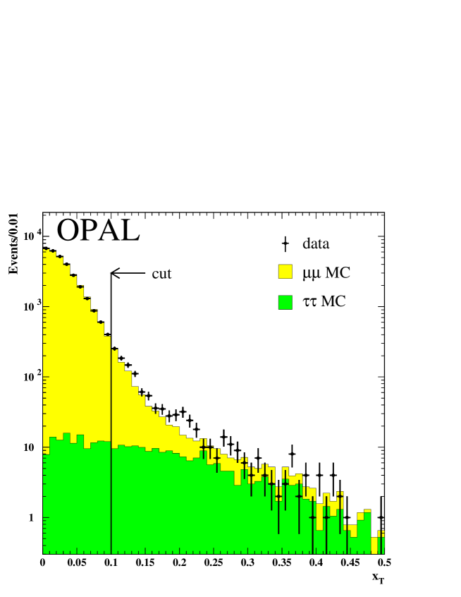
Figure 1: Distribution of selected class 1 muon pair events (as defined in subsection 5.2) vs missing transverse momentum (data points), compared to the Monte Carlo simulation of muon pair production (light histogram) and tau pair background (dark histogram). A cut $x_{T}<0.1$ accepts 96% of class 1 muon pair events and removes about 75 % of the background, which is further reduced by the tight acoplanarity cut.

where the sums are taken over respective components of the momenta of the two charged particles and the two most energetic electromagnetic clusters in the event. The cut (24) removes $\sim 75\%$ of the remaining background, as shown in fig. 1. For the asymmetry analysis described in Section 7, we also impose a strong requirement on the acoplanarity, $\xi$$<0.004$, restrict $|\cos\theta^{\bullet}|<0.92$, and limit $s^{\prime}$ to the region where the asymmetry remains the linear function of energy by imposing $\eta<0.06,0.08$ and $0.10$ at the peak$-2$, peak and peak$+2$ energy points, respectively.

These additional cuts eliminate the charge-dependent tracking problems described in [3], which lead to asymmetry biases in the subsample of poorly measured events retained for the conventional OPAL asymmetry measurements. and further reduce the $\tau$ pair background. The $\xi$-distribution is much broader for the $\tau$ pair background than for the $\mu$ pair signal, so the tight cut on acoplanarity rejects most of the remaining background events. For the asymmetry sample, used in our fits in Section 7, the estimated number of remaining $\tau\tau$ events is $25\pm 3$ out of $66143$ selected events.

As described in the next subsection, we also require that all tracks in the asymmetry sample be measured by subdetectors with optimum resolution, which retains about 62% of otherwise selected events.

5.2 Angular resolutions and muon pair event classification

It is essential for this analysis to achieve the best possible angular resolutions in both $\theta$ and $\phi$. For this reason, both muon tracks are required to have at least one hit in the central vertex detector in both axial (CVA) and stereo (CVS) planes, giving a good measurement of the production vertex. This requirement rejects about 25% of selected events. The $z$-resolution of the central jet chamber (CJ) is insufficient for this analysis, and therefore measurements are required from either the $z$-chambers or the muon chambers. This requirement rejects a further 13% of the selected events.

The azimuthal angle measurement is made by the jet chamber CJ, which determines the resolution in $\xi$. A graphical illustration of the effect of the finite $\xi$ resolution is given in fig. 2a, which shows the distribution of a subsample of events from the central region, $|\cos\theta^{\bullet}|<0.2$, with respect to the variable $\log(1/\xi)$. With a perfect detector, this distribution is expected to fall slowly and smoothly after reaching a plateau at $\log(1/\xi)\simeq 2.5-3$. With a finite resolution $\sigma_{\xi}$, all events with unmeasurably small true angular mismatch $\xi\ll\sigma_{\xi}$, which would have appeared at very high values of $\log(1/\xi)$ if the measurements were perfectly accurate, acquire larger $\xi$ of order of $\sigma_{\xi}$, and gather into the sharp peak at $\log(1/\xi)\simeq\log(1/\sigma_{\xi})\simeq 3.5$. The solid line in fig. 2a represents the result of a Gaussian fit (in $\xi$) to the data points, resulting in the estimated resolution for this subsample, $\sigma_{\xi}=0.36$ mrad, with a statistical error about 1%. The $\xi$ resolution remains virtually constant in the barrel region of the detector, $\left|\cos\theta^{\bullet}\right|<0.72$, and increases gradually to $\simeq 0.85$ mrad for $\left|\cos\theta^{\bullet}\right|>0.85$.

The resolution of the $\eta$ measurements depends on the subdetector used to measure the far ends of the two tracks in the event. CZ provides the best measurement, followed by MB, ME and, finally, CJ. The selected muon pair events are classified according to the effective resolution of $\eta$ measurement:

1. Polar angles of both tracks are determined from hits in the CZ. These events have the best resolution in $\theta$.

2. Muon chambers are used to measure both polar angles.

3. One of the tracks has its $\theta$ determined from the CZ measurement while the other is measured with the muon chambers.

4. Either or both tracks have their polar angle determined by CJ, and/or have no hits in CVA/CVS.

The distribution in $\log(1/\eta)$ of a subsample of class 1 events from the same region $|\cos\theta^{\bullet}|<0.2$ is shown in fig. 2b. Here too, the position of the peak defines the resolution of the detector. For this particular subsample, the Gaussian fit (in $\eta$), shown by the curve in fig. 2b, gives $\sigma_{\eta}=0.95\cdot 10^{-3}$, with a statistical error of about 1%. Like the $\xi$ resolution, the $\eta$ resolution increases for $\cos\theta^{\bullet}$ values outside the barrel region.

Both $\xi$ and $\eta$ resolutions were determined separately for 10 bins of $\left|\cos\theta^{\bullet}\right|$. Non-Gaussian tails were approximated by a Breit-Wigner distribution, with parameters determined from the Monte Carlo sample MC1. The $\eta$ resolution was determined separately for the different event classes defined above. Numbers of selected events in each class are shown in table 1 together with respective estimated resolutions.

	$\langle E_{\mathrm{cm}}\rangle$	Class 1	Class 2	Class 3	Class 4	Total
p$-$2	89.45 GeV	3215	1265	579	2082	7141
peak	91.22 GeV	46727	18858	9401	31244	106230
p$+$2	92.97 GeV	4853	1896	889	3147	10785
Total		54795	22019	10869	36473	124156
	Resolutions
	$\sigma_{\eta},10^{-3}$	0.95	2.0 — 3.4	1.5	2.4 — 8.0
	$\sigma_{\xi}$, mrad	0.35	0.35 — 0.85	0.35	0.35 — 2.5

Table 1: Numbers of events (prior to any cuts on angular variables $\cos\theta^{\bullet}$, $\eta$ and $\xi$, but after all other cuts) and estimated resolutions in $\eta$ and $\xi$ for the three energy points and various classes of events as defined in the text. Events from classes 1 and 3 are from the barrel region of the detector, $|\cos\theta^{\bullet}|<0.72$; most of class 2 events belong to the region $0.72<|\cos\theta^{\bullet}|<0.92$. For classes 2 and 4 the resolutions depend on the polar angle: the smaller numbers for the resolutions $\sigma_{\eta}$, $\sigma_{\xi}$ correspond to $|\cos\theta^{\bullet}|\gtrsim 0.72$, while the larger numbers refer to the edge of acceptance $|\cos\theta^{\bullet}|\lesssim 0.92$.

Only events from classes 1 and 2 are used in our main analysis (adding up to about 62 % of the selected muon pair events remaining after the cut on missing transverse energy), with class 3 events used for systematic studies. The $\eta$ resolution for events from class 4 was found to be non-uniform with respect to the polar angle and generally poor, so that they could not be used.

6 $\cos\theta^{\bullet}$ distributions for various $\eta$, $\xi$ regions

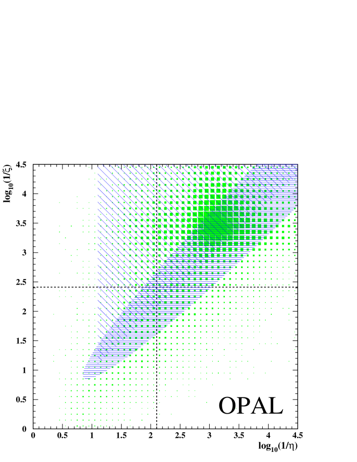
Figure 3: Distribution of class 1 events in the $\log(1/\xi)-\log(1/\eta)$ plane. Events from the lightly shaded triangular area above the diagonal have a high ISR probability, while the densely shaded area along the diagonal contains events with a high probability of significant FSR and/or IFI. The horizontal dashed line represents the cut on acoplanarity angle $\xi_{0}=0.004$, while the vertical dashed line corresponds to $\eta=0.008$.

The scatter plot of the class 1 events in the $\log(1/\eta)-\log(1/\xi)$ plane is shown in fig. 3. As explained above, the events placed along the diagonal of this plot, corresponding to $\eta\sim\xi$ (area with dense horizontal shading), have a high probability of strong FSR and/or IFI. Events with $\eta\gg\xi$, scattered above the diagonal (diagonally shaded triangular area in fig. 3) typically have a high probability of significant ISR. As in fig. 2, the position of the peak in fig. 3 is determined by the detector resolution in $\eta$ and $\xi$. Class 2 events show a very similar scatter plot, apart from the fact that, because of the inferior resolution, the peak is shifted towards higher values of $\xi$ and $\eta$ (i.e. down along the diagonal of the plot in fig. 3).

A cut on acoplanarity $\xi_{0}=0.004$, corresponding to $\log_{10}(1/\xi)\approx 2.4$, is shown in fig. 3 by the horizontal dashed line. The vertical dashed line corresponds to $\eta=0.008$, $\log_{10}(1/\eta)\approx 2.1$. This value was chosen to separate the area of relatively large $\eta$ values, where the finite $\eta$-resolution effects are not too important, and the region of small $\eta$, where the distributions are significantly smeared by the detector resolution.

The upper-left quadrant in fig. 3 is filled with events with small $\xi$ ($\xi<0.004$) and large $\eta$ ($\eta>0.008$). In this kinematic range there is a high probability of strong ISR, but it is essentially free of IFI and FSR contributions. Thus the distribution of the events from this quadrant in $\cos\theta^{\bullet}$ should be well described by the usual quadratic function of $\cos\theta^{\bullet}$, eq. (21).

The upper right quadrant in fig. 3 contains events with both $\xi$ and $\eta$ small. Here the IFI contribution is expected to be strong and should lead to an additional logarithmic dependence on $\cos\theta^{\bullet}$, described by the second term in curly brackets in eq. (22). This dependence gives rise to an additional, IFI-induced forward-backward asymmetry, which is expected to be positive in this part of the $\eta$–$\xi$ plane.

The lower left quadrant of fig. 3 also contains a strong IFI contribution, but in this region the IFI-induced asymmetry is expected to be negative. Theory predicts that, when integrated over the whole range of $\xi$ and $\eta$, these positive and negative logarithmic interference terms cancel each other so that the overall $\cos\theta^{\bullet}$ distribution is again described well by a simple quadratic function of $\cos\theta^{\bullet}$, with the only asymmetric term being linear in $\cos\theta^{\bullet}$.

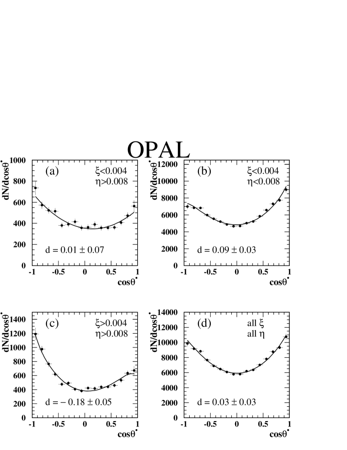
Figure 4: $\cos\theta^{\bullet}$-distributions for the class 1 and class 2 events at ${\mathrm{Z}}$ peak, integrated over separate areas of the $\log(1/\xi)-\log(1/\eta)$ plane from fig. 3, together with fit results using the function (25): a) upper left quadrant, where the asymmetry is dominated by the linear term ($d\simeq 0$); b) upper right quadrant, where the IFI-induced asymmetry is significant and positive ($d>0$); c) lower left quadrant, where the IFI-induced asymmetry is large and negative ($d<0$); d) the whole plane, where the IFI contribution is compatible with zero as a result of the cancellation.

Figs. 4a–d show the $\cos\theta^{\bullet}$-dependence for class 1 and class 2 events collected at the ${\mathrm{Z}}$ peak. The measured distributions were corrected for efficiency and background using the $\mu\mu$ and $\tau\tau$ Monte Carlo samples including full detector simulation. Figs. 4a–c correspond to upper left, upper right and lower left quadrants of fig. 3 respectively, while fig. 4d shows the $\cos\theta^{\bullet}$ distribution integrated over the whole $\eta$–$\xi$ plane. Also shown are fits to the measured distributions using the following function:

$${}(a+b\cos\theta^{\bullet}+c\cos^{2}\theta^{\bullet})\bigl{(}1+d{{1}\over{2}}\ln{{1+\cos\theta^{\bullet}}\over{1-\cos\theta^{\bullet}}}\bigr{)}.$$ (25)

which is merely a simplified version of eq. (22) after the integration over the respective quadrant of the $\eta$–$\xi$ plane. Among the four fit parameters in (25), $a,b,c$ and $d$, the last one, $d$, is particularly interesting, as it determines the amount of the IFI-induced forward-backward asymmetry. Its fitted values are shown in the figure for each of the four distributions.

These fit results clearly demonstrate that theoretical expectations are fulfilled: the $\cos\theta^{\bullet}$-distribution of the events taken from the upper left quadrant of fig. 3 is indeed well described by a quadratic function, giving $d=0.01\pm 0.07$, compatible with the absence of IFI contribution. On the contrary, events from the two quadrants situated along the diagonal of fig. 3 both show a significant non-zero IFI contribution: the upper right quadrant yields a positive IFI-induced asymmetric term, $d=0.09\pm 0.03$, while the lower left quadrant (events with both $\xi$ and $\eta$ large) yields a negative value, $d=-0.18\pm 0.05$. Most notably, when all regions of $\eta$ and $\xi$ are summed, the resulting $\cos\theta^{\bullet}$ distribution in fig. 3d, with $d=0.03\pm 0.03$, is again compatible with the absence of the IFI-induced logarithmic term.

Before moving on to the detailed quantitative analysis of the measured angular distributions, let us show that the differences in the asymmetric parts of the measured $\cos\theta^{\bullet}$ distributions in different $\eta$–$\xi$ regions are indeed caused by the initial-final radiation interference. Consider the “differential forward-backward asymmetry”, defined by

$$A_{FB}(\cos\theta^{\bullet})\equiv{{{{d\sigma(\cos\theta^{\bullet})}\over{d\cos\theta^{\bullet}}}-{{d\sigma(-\cos\theta^{\bullet})}\over{d\cos\theta^{\bullet}}}}\over{{{d\sigma(\cos\theta^{\bullet})}\over{d\cos\theta^{\bullet}}}+{{d\sigma(-\cos\theta^{\bullet})}\over{d\cos\theta^{\bullet}}}}},$$ (26)

as a function of $\cos\theta^{\bullet}$, for the same three separate areas of the $\log(1/\xi)-\log(1/\eta)$ plane considered above. This is compared to two Monte Carlo samples, MC1 and MC2, as defined in Section 4. MC1 has the IFI term switched off, while MC2 includes the IFI contribution.

Fig. 5a represents the upper left corner of fig. 3, rich with ISR, and shows a negative asymmetry with the smooth angular dependence $\sim\cos\theta^{\bullet}/(1+\cos^{2}\theta^{\bullet})$, typical of the linear term. The two lines, corresponding to the Monte Carlo samples with and without initial-final interference, display no significant differences, and both describe the data well.

In contrast, the shape of the angular dependence for the upper right (fig. 5b) and lower left (fig. 5c) quadrants is dominated by the logarithmic term $\sim\ln[(1+\cos\theta^{\bullet})/(1-\cos\theta^{\bullet})]$, characteristic of the IFI-induced forward-backward asymmetry. The data and the MC2 sample agree reasonably well, while for the MC1 this is not the case.

When integrated over the whole $\eta$-$\xi$ plane, the angular dependence is essentially symmetric, as shown in fig. 5d, without any significant deviation between the data and either Monte Carlo sample.

7 Asymmetry analysis

7.1 Probability density

As mentioned above, a tight cut on acoplanarity selects an area of phase space where we can apply the formalism presented in section 3, measure the energy dependence of the forward-backward asymmetry and determine the vector and axial-vector couplings of ${\mathrm{Z}}$. Based on the expression (22) for the double-differential cross section, one obtains the following probability density function:

$${\cal P}(\eta,\cos\theta^{\bullet})\sim\Bigl{\{}\;{3\over 8}\;(1+\cos^{2}\theta^{\bullet})+\Bigl{[}A_{0}+A^{\prime}{{s^{\prime}-M_{Z}^{2}}\over{s}}\Bigr{]}\;\cos\theta^{\bullet}\Bigr{\}}$$

$$\times f_{+}(\eta)\Bigl{\{}1+\beta(\eta,\cos\theta^{\bullet})+B\,{{f_{-}(\eta)}\over{f_{+}(\eta)}}\,{{1}\over{2}}\ln{{1+\cos\theta^{\bullet}}\over{1-\cos\theta^{\bullet}}}\Bigr{\}}$$ (27)

where $A_{0}$, $A^{\prime}$ and $B$ are constants to be determined from a fit to the data. $A_{0}$ and $A^{\prime}$ correspond to the coupling combination terms in equation (18). In the single soft photon approximation of QED one expects $B=1$, so by measuring $B$ we can accommodate and measure deviations from this approximation.

The function $f_{+}(\eta)$ essentially defines the shape of the $\eta$-dependence of the cross section, and was measured directly from the data. Indeed, the single-differential distribution with respect to $\eta$, obtained by integrating the probability density (7.1) over the whole $\cos\theta^{\bullet}$ range, is essentially proportional to the function $f_{+}(\eta)$. The corrections from the FSR contribution $\beta$, defined in eq. (23), and the product of the two terms in eq. (7.1) which are odd functions of $\cos\theta^{\bullet}$  are fairly small and can be easily taken into account.

Before application to the data, $\eta$ resolution smearing must be explicitly applied to (7.1). Note that the $\eta$ dependence enters not only through $f_{\pm}$, but also through $s^{\prime}$ within the first pair of curly brackets, so the probability distribution folded with the resolution is no longer factorisable. However, the $\eta$-dependence of the first term is linear, so one only needs to calculate three different ratios of folded functions: $\Psi_{1}(\eta)={\overline{f_{-}(\eta)}}/{\overline{f_{+}(\eta)}}$, $\Psi_{2}(\eta)={\overline{\eta f_{-}(\eta)}}/{\overline{f_{+}(\eta)}}$ and $\Psi_{3}(\eta)={\overline{\eta f_{+}(\eta)}}/{\overline{f_{+}(\eta)}}$, where ${\overline{f}}$ denotes a function $f$ convoluted with the $\eta$-resolution. These three ratios are presented in fig. 6, together with similar ratios without resolution smearing. Even the largest of these three ratios, $\Psi_{1}={\overline{f_{-}}}/{\overline{f_{+}}}$, which essentially determines the IFI contribution to the asymmetry, is much smaller than 1 at $\eta\simeq 0$ and quickly becomes even smaller outside a narrow range of $\eta$, the width of which is governed by the cut on $\xi$ and the resolution in $\eta$.

Since the standard OPAL selection efficiency for $\mu$-pair events is very close to 100%, the efficiency of the class 1 and 2 selections can be determined directly from the data. Fig. 7 shows the ratios, $\varepsilon_{i}(\cos\theta^{\bullet})$, of class 1 and class 2 events to events of all classes, as a function of $\cos\theta^{\bullet}$, for events passing all other requirements for the asymmetry sample, including cuts on $x_{T}$, $\xi$, $\eta$ and $\cos\theta^{\bullet}$. The small inefficiencies due to the $x_{T}$ requirement and resolution losses in the $\xi$ cut are calculated using the Monte Carlo, as described in the Appendix.

Finally, the expected probability distributions (7.1) summed over event classes, convoluted with the respective $\eta$ resolutions and appropriately weighted with the respective efficiencies, are normalised so that the total probability is independent of the fit parameters. The resulting formula, incorporating all the corrections described above, is given in the Appendix.

It is convenient to re-express the asymmetry at peak, $A_{0}$, and the slope of the asymmetry with energy, $A^{\prime}$, in terms of the vector and axial-vector couplings of the Z, as in (18), and use the following set of fit parameters:

$${}p_{1}={{|g_{V}|}\over{|g_{A}|}},\;\;\;p_{2}={{|g_{A}|}\over{\sqrt{K}}},\;\;\;p_{3}=B.$$ (28)

The first two parameters have obvious physical meanings, while the last determines the measured intensity of the IFI-induced term, compared to the single soft photon approximation. The asymmetry at peak and the slope now read:

$$A_{0} \equiv A_{FB}(M_{Z}^{2})=3\,p_{1}^{2}/(1+p_{1}^{2})^{2}+A_{\gamma},$$ (29)

$$A^{\prime} \equiv A^{\prime}_{FB}(M_{Z}^{2})=3\,(1/p_{2})^{2}/(1+p_{1}^{2})^{2},{}$$ (30)

where $A_{\gamma}=0.002$ is the offset to the pole asymmetry due to the imaginary part of the photon propagator.

7.2 Results

An unbinned maximum likelihood fit is made using the data sample from classes 1 and 2, with the probability density function and the set of parameters described in the previous subsection. The cut on acoplanarity is chosen to be $\xi_{0}=0.004$, which is found to be small enough to reject most of the FSR contribution and justify the soft photon approximation, while simultaneously being large enough compared to the $\xi$ resolution. The range of $\cos\theta^{\bullet}$ used in the fit is limited by the acceptances of relevant subdetectors to $-0.92<$$\cos\theta^{\bullet}$$<0.92$, while the upper bound for the variable $\eta$, $\eta_{\mathrm{max}}$, is limited by the range of $s^{\prime}$ where the asymmetry is expected to be a linear function of energy. We choose $\eta_{\mathrm{max}}=0.06,\ 0.08,\ 0.10$ for data taken at peak$-2$, peak and peak$+2$, respectively. This upper bound for $\eta$  removes about 0.1% of the remaining events.

Table 2 presents fit results for peak data only, for peak$-2$ and peak$+2$ simultaneously, and for all three energy points simultaneously. The errors shown in the table are statistical only. The corresponding correlation matrices are given in table 3. No meaningful results have been obtained for peak$-2$ or peak$+2$ data sets separately, because of the limited statistics at these energies.

$E_{\mathrm{cm}}$	$|g_{V}/g_{A}|$	$|g_{A}|/\sqrt{K}$	B
${\mathrm{Z}}$ peak	$0.0830\pm 0.0125$	$0.6013\pm 0.0314$	$0.811\pm 0.129$
p$-$2 & p$+$2	$0.0720\pm 0.0312$	$0.6226\pm 0.0212$	$0.952\pm 0.322$
All energies	$0.0795\pm 0.0114$	$0.6165\pm 0.0177$	$0.840\pm 0.120$

Table 2: Fit results for various energy combinations. Errors are statistical only.

${\mathrm{Z}}$ peak	$|g_{V}/g_{A}|$	$|g_{A}|/\sqrt{K}$	B
$|g_{V}/g_{A}|$	1.000	-0.396	-0.698
$|g_{A}|/\sqrt{K}$	-0.396	1.000	0.190
B	-0.698	0.190	1.000
p-2 & p+2	$|g_{V}/g_{A}|$	$|g_{A}|/\sqrt{K}$	B
$|g_{V}/g_{A}|$	1.000	-0.186	-0.663
$|g_{A}|/\sqrt{K}$	-0.186	1.000	0.113
B	-0.663	0.113	1.000
All energies	$|g_{V}/g_{A}|$	$|g_{A}|/\sqrt{K}$	B
$|g_{V}/g_{A}|$	1.000	-0.261	-0.694
$|g_{A}|/\sqrt{K}$	-0.261	1.000	0.133
B	-0.694	0.133	1.000

Table 3: Correlation matrices for the three fits.

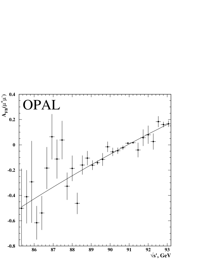
Figure 8: Fitted asymmetry in narrow slices of $\sqrt{s^{\prime}}$, with the initial-final radiation interference term fixed to its value measured in this analysis, $B=0.840$.

The unbinned maximum likelihood fit does not give any goodness-of-fit parameter for judging the quality of the fit. In order to do this and to illustrate our results graphically, we subdivide the data into 30 bins in $\sqrt{s^{\prime}}$, and perform a single parameter maximum likelihood fit in each bin (with $B$ fixed to its previously determined value, $B=0.840$) for the coefficient of the $\cos\theta^{\bullet}$ term in eq. (7.1). The results are presented in fig. 8. One sees that the measured asymmetry at various $\sqrt{s^{\prime}}$ values are indeed aligned close to a straight line, whose value at ${s^{\prime}}=M_{Z}^{2}$ and slope can now be determined from a minimum $\chi^{2}$ fit to these points. The fitted line is also shown in fig. 8. The value of $\chi^{2}/$d.o.f.$=38.9/28$ suggests that the fit quality is acceptable. The results of this fit:

$$\Bigl{|}{{g_{V}}\over{g_{A}}}\Bigr{|}=0.0813\pm 0.0082,\;\;\;\Bigl{|}{{g_{A}}\over{\sqrt{K}}}\Bigr{|}=0.6246\pm 0.0184$$ (31)

are in agreement with the results of our main fit from table 2. The smaller error in (31) is due to the fact that the parameter $B$ was fixed; fixing $B$ in the maximum likelihood fit also results in smaller errors, 0.0082 and 0.0175, respectively.

7.3 Systematic Studies

The probability density function used in the fit depends upon a number of parameters whose values cannot be precisely fixed. The variation of fit results due to varying these parameters within a reasonable range allows one to estimate corresponding systematic errors.

Various sources of systematic error have been considered, and the resulting errors are summarised in table 4, for the data taken at the Z peak only, and for all three energies analysed simultaneously.

1. The fit was repeated with an additional cut $|$$\cos\theta^{\bullet}$$|<0.90$, to check sensitivity against the variation of the edge of the geometric acceptance. The assigned systematic error is the absolute value of the shift, wherever the shift is statistically significant, plus a small contribution due to the uncertainty of the absolute scale of the $\cos\theta^{\bullet}$ measurement.

2. The parameters $\sigma_{\eta}$, describing the experimental resolution in the $\eta$ measurement, and determined from the data in bins of $\cos\theta^{\bullet}$ for various classes of events, were scaled by a factor of $1\pm 0.1$ for each class separately. The assigned systematic error is the largest of the absolute values of the observed shifts.

3. The calculations involving the function $f_{-}(\eta)$ are less reliable for $\eta\gtrsim\Gamma_{Z}/(2M_{Z})$, where the photon spectrum can be affected by the ${\mathrm{Z}}$ resonance lineshape. To study the influence of this uncertainty, the fit was repeated with $f_{-}(\eta)$ set to zero for $\eta>0.010$. The assigned systematic error is the absolute value of the shift.

4. In order to check for possible biases due to the approximations made in deriving eq. (18), the fit was repeated with next-to-leading terms in $\eta$ taken into account. The assigned systematic error is the absolute value of the shift.

5. Monte Carlo studies have shown that deviations from the equation $s^{\prime}=s(1-2\eta)$ within the angular range considered here do not exceed $\pm 0.5\%$. Possible biases were checked by replacing $\eta$ with $\delta_{1}+(1+\delta_{2})\eta$, where $\delta_{1,2}=\pm 0.5\%$. The assigned systematic error is the largest of the absolute values of the shifts.

		Z peak			All energies
	Variation	$|g_{V}/g_{A}|$	$|g_{A}|/\sqrt{K}$	B	$|g_{V}/g_{A}|$	$|g_{A}|/\sqrt{K}$	B
1	$|\cos\theta^{\bullet}|<0.90$	0.0014	0.0000	0.054	0.0002	0.0000	0.062
2	$\sigma_{\eta}$	0.0005	0.0009	0.002	0.0006	0.0002	0.002
3	$f_{-}(\eta)$ tail	0.0001	0.0038	0.001	0.0006	0.0012	0.003
4	$s^{\prime}$-dependence	0.0005	0.0053	0.004	0.0007	0.0018	0.001
5	$s^{\prime}\leftrightarrow\eta$ relation	0.0001	0.0015	0.001	0.0001	0.0016	0.001
	Total syst.	0.0016	0.0068	0.054	0.0011	0.0027	0.063
	Stat. error	0.0125	0.0314	0.129	0.0114	0.0177	0.120
	Total error	0.0126	0.0321	0.140	0.0115	0.0179	0.136

Table 4: Various contributions to the systematic errors, for the data taken at the Z peak only, and for all three energy points.

The total systematic uncertainty for each fit parameter was calculated as a quadratic sum of the partial contributions.

The following checks have also been made:

• The fit was repeated with an additional cut to remove data in the range $0.70<|$$\cos\theta^{\bullet}$$|<0.75$, to exclude the edge of the barrel part of the detector.

• The acoplanarity cut $\xi_{0}$ was varied by $\pm 0.001$ from its central value of 0.004.

• The upper limit of the $\eta$ range was varied by $\pm 0.010$ from its central value for each energy point.

• The number of bins in the measured $\eta$-dependence was changed by $\pm 10$ from its default value of 50.

• In order to check the reliability of the efficiency calculation, class 3 events (defined in subsection 5.2) were added to the analysis.

• The number of bins in the measured efficiency as a function of $\cos\theta^{\bullet}$ was changed by $\pm 50$ from its default value of 100.

• The cut on the missing transverse energy (24) was tightened from 0.10 to 0.05, effectively reducing the $\tau$ pair background contribution by a factor of 2.

In all these cases, the observed shifts were well within expected statistical variations, each of which constituted a fraction of the total statistical error, therefore no additional systematic errors were assigned.

7.4 Determination of $g_{V}$, $g_{A}$ and $\sin^{2}\theta_{W}$

Combining statistical and systematic errors, for the results at all three energy points we obtain:

$$\ \Bigl{|}{{g_{V}}\over{g_{A}}}\Bigr{|} = 0.0795\pm 0.0115$$ (32)

$$\Bigl{|}{{g_{A}}\over{\sqrt{K}}}\Bigr{|} = 0.6165\pm 0.0179$$ (33)

$$B = 0.840\pm 0.136.$$ (34)

These results are essentially independent of SM assumptions and SM parameter values. The only assumptions used are those of QED, electron-muon universality and the spin-1 nature of ${\mathrm{Z}}$.

For comparison, the values for the quantities (32) and (33), extracted from the ratios $C^{a}_{ZZ}/C^{s}_{ZZ}$ and $C^{a}_{\gamma Z}/C^{s}_{ZZ}$, as measured in the conventional asymmetry analysis [3] using the full OPAL muon data sample of 1990-1995, are:

$$\ \Bigl{|}{{g_{V}}\over{g_{A}}}\Bigr{|} = 0.0713\pm 0.0055$$ (35)

$$\Bigl{|}{{g_{A}}\over{\sqrt{K}}}\Bigr{|} = 0.6178\pm 0.0147.$$ (36)

These two sets of numbers are in agreement with each other, as well as with the SM expectations :

$$\ \Bigl{|}{{g_{V}}\over{g_{A}}}\Bigr{|} = 0.0729^{+0.0015}_{-0.0043}$$ (37)

$$\Bigl{|}{{g_{A}}\over{\sqrt{K}}}\Bigr{|} = 0.59459^{+0.00047}_{-0.00013}.$$ (38)

The measured value of $B$, eq. (34), is also compatible with the expectation, $B=1$, of the single soft photon approximation.

From the measured ratio $|g_{V}/g_{A}|$ we can directly determine the effective weak mixing angle in the Standard Model (assuming that $g_{V}$ and $g_{A}$ have the same signs):

$$\sin^{2}\theta_{W}^{\mathrm{eff}}\equiv{{1}\over{4}}\Bigl{(}1-{{g_{V}}\over{g_{A}}}\Bigr{)}=0.2301\pm 0.0029,$$ (39)

which is in agreement with the world average $0.23150\pm 0.00016$ [9]. In order to determine the effective couplings $g_{V}$ and $g_{A}$ separately, we have to substitute numerical values (which are well measured elsewhere [9] in the context of the Standard Model) into the definition of the normalization constant $K$ (eq. (19)). Using (20), one gets $\sqrt{K}=0.843108$, which gives the following values for the vector and axial-vector couplings of the ${\mathrm{Z}}$ boson:

$$\bigl{|}{g_{V}}\bigr{|} = 0.0413\pm 0.0060,$$

$$\bigl{|}{g_{A}}\bigr{|} = 0.520\pm 0.015.$$ (40)

The higher precision of the conventional analysis is mostly due to its higher statistics, since this analysis is restricted to events with accurate angular measurements. However, in contrast with the conventional analysis, this analysis has the ability of extracting the slope of the energy dependence of the asymmetry (and hence the parameter $g_{A}$) from the data taken at a single energy point. By comparing the errors on the parameter $g_{A}/\sqrt{K}$ determined from the peak and off-peak data in Table 2 one can see that the weight of the peak contribution to the final precision is quite significant. This information is clearly complementary to the standard analysis, and can be combined with the results of the latter to improve the overall precision on the relevant coefficient, $C^{a}_{\gamma Z}$. The values for these coefficients from the standard OPAL analysis [3], from muon data only, and averaged over the three lepton flavours,

$$C^{a}_{\gamma Z}(\mu^{+}\mu^{-})=0.232\pm 0.011,\;\;\;\;\;\;\;\;C^{a}_{\gamma Z}(l^{+}l^{-})=0.2350\pm 0.0080,$$ (41)

can be combined with the value obtained, using eq. (16), from this analysis (Z peak only):

$$C^{a}_{\gamma Z}(\mu^{+}\mu^{-})=0.257\pm 0.027.$$ (42)

We obtain:

$$C^{a}_{\gamma Z}(\mu^{+}\mu^{-})=0.236\pm 0.010,\;\;\;\;\;\;\;\;C^{a}_{\gamma Z}(l^{+}l^{-})=0.2368\pm 0.0077,$$ (43)

which now represent the best OPAL values for these coefficients.

8 Conclusion and outlook

We have analysed the angular dependence of muon pair production in electron-positron annihilation at centre of mass energies near the ${\mathrm{Z}}$ peak, using various angular variables. Our approach is novel in a number of respects. The usual procedure involves the integration over the phase space of the radiated photons, limited by a cut on acollinearity (eq. (8)). In contrast, we measure small angular mismatches between the directions of the two final muons, separately in the polar ($\eta$) and azimuthal ($\xi$) directions, and use them to determine the influence of the initial and final state photon radiation and their interference. Effects of final state photon radiation are removed by applying a tight cut on the acoplanarity, $\xi$. The contribution of the additional asymmetric term arising as a result of this cut is measured through its specific polar angle dependence. The variable $\eta$ is used to assess the energy of the radiated photon and to determine the variation of the forward-backward asymmetry with the invariant mass of the muon pair, which is shown to be linear in the vicinity of the ${\mathrm{Z}}$ peak (see fig. 8).

By using a well-behaved variable, $\cos\theta^{\bullet}$, instead of the polar angle of one of the muons, and explicitly incorporating the initial-final interference into the fit, we significantly reduce the dependence of the measured asymmetry upon the polar angle acceptance cut.

The measured values presented in equations (32–34) are directly obtained from the data; they can be compared to those of other experiments, or to theoretical models. By substituting the SM value for the constant $K$, we get results for $g_{V}$, $g_{A}$ and the effective weak mixing angle compatible with those obtained with the analyses based on the assumptions of the Standard Model. The statistical precision of our result, while obviously inferior to that of the model dependent analysis when applied to many channels, is comparable with the precision of a conventional analysis which just uses the data from the muon pair asymmetry (there is some loss of statistical power due to the more restrictive requirements for events with accurate angular measurements).

We have also demonstrated that the effect of IFI is adequately described by the leading order QED corrections, and that the asymmetry does vary greatly with the angular cut imposed, showing that, while the correction to a conventional analysis which integrates over all photon phase space is small, this is because of a large cancellation which requires respectful treatment.

In experiments at proposed future electron-positron colliders [21], the collisions between the very dense bunches will produce radiation and lower the effective CM energy. This effect is similar to ISR, but depends not only on a standard QED radiator function but also on the detailed bunch dynamics, which can vary from one collision to the next. This presents a serious challenge for conventional muon pair analysis at such machines, whereas this method is not disturbed by such a variation.

9 Appendix

The full expression for the probability density used in the unbinned likelihood fit has the following form:

$${\cal P}(\eta,z)={{1}\over{\cal N}}\,\varepsilon_{\xi}(|z|)\,\varepsilon_{t}(|z|)\,\sum_{i}\varepsilon^{i}(z)\,\rho^{i}(s,\eta)\sum_{j=1}^{9}D_{j}^{i}(\eta)\,H_{j}(z)$$ (44)

where $H_{j}$ stand for different types of dependence upon $z\equiv$$\cos\theta^{\bullet}$:

$$H_{1} = {{3}\over{8}}(1+z^{2})$$

$$H_{2} = {{3}\over{8}}(1+z^{2})\,{{1}\over{4z}}\ln{{1+z}\over{1-z}}$$

$$H_{3},\,H_{4} = z\,{{1}\over{2}}\ln{{1+z}\over{1-z}}$$

$$H_{5},\,H_{6} = z$$ (45)

$$H_{7},\,H_{8} = z\,{{1}\over{4z}}\ln{{1+z}\over{1-z}}$$

$$H_{9} = {{3}\over{8}}(1+z^{2})\,{{1}\over{2}}\ln{{1+z}\over{1-z}}$$

Coefficients $D_{1}^{i}$ — $D_{9}^{i}$ are expressed through constants $A_{0}$, $A^{\prime}$, $B$, defined in eqs. (28–30), and the ratios, $\Psi_{1},\Psi_{2},\Psi_{3}$, of the convoluted functions $f_{\pm}$:

$$D_{1}^{i} = 1$$

$$D_{2}^{i} = \Psi_{1}^{i}(\eta)$$

$$D_{3}^{i} = [A_{0}+A^{\prime}(s-M_{Z}^{2})/(2s)]\,B\,\Psi_{1}^{i}(\eta)$$

$$D_{4}^{i} = -A^{\prime}\,B\,\Psi_{2}^{i}(\eta)\,$$

$$D_{5}^{i} = [A_{0}+A^{\prime}(s-M_{Z}^{2})/(2s)]$$ (46)

$$D_{6}^{i} = -A^{\prime}\,\Psi_{3}^{i}(\eta)\,$$

$$D_{7}^{i} = [A_{0}+A^{\prime}(s-M_{Z}^{2})/(2s)]\,\Psi_{1}^{i}(\eta)$$

$$D_{8}^{i} = -A^{\prime}\,\Psi_{2}^{i}(\eta)\,$$

$$D_{9}^{i} = B\,\Psi_{1}^{i}(\eta)$$

where

$$\Psi_{1}^{i}(\eta)={{\overline{f_{-}(\eta)}}\over{\overline{f_{+}(\eta)}}},\;\;\;\;\Psi_{2}^{i}(\eta)={{\overline{\eta f_{-}(\eta)}}\over{\overline{f_{+}(\eta)}}},\;\;\;\;\Psi_{3}^{i}(\eta)={{\overline{\eta f_{+}(\eta)}}\over{\overline{f_{+}(\eta)}}},$$ (47)

with the horizontal bar denoting resolution smearing. The index $i$ serves as a reminder that the resolution parameter $\sigma^{i}_{\eta}$, used during the smearing, is different for different event classes $i$. Note that the functions $\Psi_{k}^{i}(\eta)$ also implicitly depend on the acoplanarity cut $\xi_{0}$.

The factor $\varepsilon_{\xi}(|z|)$ stands for the selection probability of an event with a true acoplanarity $\xi^{\mathrm{true}}<\xi_{0}$ when the cut is applied on the measured acoplanarity $\xi$ of the event. It was determined using the MC1 sample, and is within $\sim 10^{-3}$ of unity when $\sigma_{\xi}\ll\xi_{0}$ (which is the case for the barrel region $|z|<0.7$), decreasing slightly for larger $z$, where the $\xi$ resolution is worse.

Similarly, the factor $\varepsilon_{t}(|z|)$ takes into account the variation of efficiency with $|$$\cos\theta^{\bullet}$$|$ due to the cut on the missing transverse energy, eq. (24). It also was determined using the MC1 sample, and decreases from $\sim 96\%$ in the barrel region to $\sim 80\%$ at the edge of the acceptance.

$\varepsilon^{i}(z)$ is the class-specific selection efficiency relative to the total efficiency for all classes, including those not used in present analysis, and is determined directly from the data (Fig. 7). So are the functions $\rho^{i}(s,\eta)$ which, for a particular class $i$ at each initial energy point $\sqrt{s}$, are essentially equal to the measured $\eta$-distributions, dominated by the $j=1$ term in eq. (44), with small and calculable corrections from other terms in the sum.

Finally, the normalisation constant ${\cal N}$ is determined from the condition that the total probability is equal to 1.

Acknowledgements:

We particularly wish to thank the SL Division for the efficient operation of the LEP accelerator at all energies and for their continuing close cooperation with our experimental group. We thank our colleagues from CEA, DAPNIA/SPP, CE-Saclay for their efforts over the years on the time-of-flight and trigger systems which we continue to use. In addition to the support staff at our own institutions we are pleased to acknowledge the
Department of Energy, USA,
National Science Foundation, USA,
Particle Physics and Astronomy Research Council, UK,
Natural Sciences and Engineering Research Council, Canada,
Israel Science Foundation, administered by the Israel Academy of Science and Humanities,
Minerva Gesellschaft,
Benoziyo Center for High Energy Physics,
Japanese Ministry of Education, Science and Culture (the Monbusho) and a grant under the Monbusho International Science Research Program,
Japanese Society for the Promotion of Science (JSPS),
German Israeli Bi-national Science Foundation (GIF),
Bundesministerium für Bildung und Forschung, Germany,
National Research Council of Canada,
Research Corporation, USA,
Hungarian Foundation for Scientific Research, OTKA T-029328, T023793 and OTKA F-023259.

Figure 2: Distribution of class 1 events from the central region $\left|\cos\theta^{\bullet}\right|<0.2$ with respect to the variables $\log(1/\xi)$ (a) and $\log(1/\eta)$ (b). The positions of the peaks, shown by the arrows, determine the experimental resolutions in $\xi$ and $\eta$.

Figure 5: Differential asymmetry defined in eq. (26) for the class 1 and class 2 events at ${\mathrm{Z}}$ peak, corresponding to four different areas of the $\log(1/\xi)-\log(1/\eta)$ plane from fig. 3: upper left quadrant (a), where the asymmetry is dominated by the linear term; upper right quadrant (b), where the positive IFI-induced asymmetry is dominant; lower left quadrant (c), where the IFI-induced asymmetry is large and negative; and the whole plane (d), with no significant asymmetry of any kind. Data points with error bars represent OPAL data, the solid histogram shows the MC1 sample without the IFI contribution, while the dashed histogram shows the MC2 sample which contains IFI.

Figure 6: Typical dependence of the ratios $\Psi_{1}(\eta)={\overline{f_{-}(\eta)}}/{\overline{f_{+}(\eta)}}$ (a), $\Psi_{2}(\eta)={\overline{\eta f_{-}(\eta)}}/{\overline{f_{+}(\eta)}}$ (b) and $\Psi_{3}(\eta)={\overline{\eta f_{+}(\eta)}}/{\overline{f_{+}(\eta)}}$ (c) on $\eta$ before (dashed lines) and after (solid lines) convoluting each of the functions with the $\eta$ resolution. In this example, the acoplanarity cut is $\xi_{0}=0.004$, while the $\eta$ resolution parameter is $\sigma_{\eta}=0.002$.

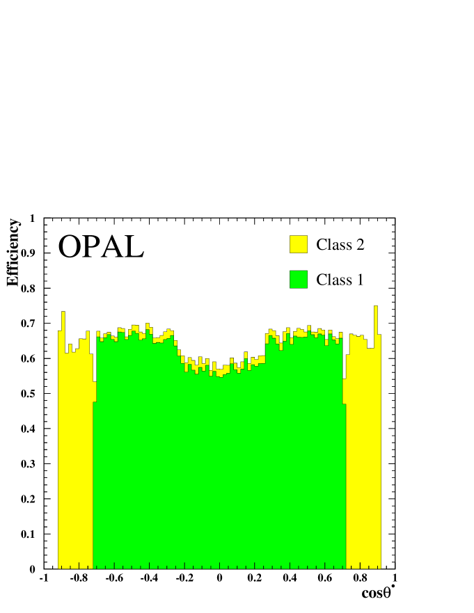
Figure 7: Selection efficiencies for classes 1 (dark histogram) and 2 (light histogram) as functions of $\cos\theta^{\bullet}$, as determined from the sample of events passing all cuts for the asymmetry sample, including those on $x_{T}$, $\xi$, $\eta$ and $\cos\theta^{\bullet}$.

References

-
[1]
CELLO Collab., H. J. Behrend et al., Phys. Lett. B191 (1987) 209;
JADE Collab., W. Bartel et al., Phys. Lett. B108 (1982) 140;
MARK J Collab., B. Adeva et al., Phys. Rev. Lett. 48 (1982) 1701;
PLUTO Collab., C. Berger et al., Z. Phys. C27 (1985) 249;
TASSO Collab., R. Brandelik et al., Phys. Lett. B110 (1982) 173;
VENUS Collab., M. Miura et al., Phys. Rev. D57 (1998) 5345. -
[2]
ALEPH Collab., R. Barate et al., Euro. Phys. J. C14 (2000) 1;
DELPHI Collab., P. Abreu et al., Euro. Phys. J. C16 (2000) 371;
L3 Collab., M. Acciarri et al., Euro. Phys. J. C16 (2000) 1;
SLD Collab., K. Abe et al., Phys. Rev. Lett. 86 (2001) 1162. - [3] OPAL Collab., G. Abbiendi et al., Euro. Phys. J. C19 (2001) 587.
- [4] See, e.g., G.Altarelli in Physics at LEP, CERN Yellow Report 86-02, Vol. 1, p. 3, Geneva, 1986, and references therein.
- [5] F. A. Berends, K. J. F. Gaemers and R. Gastmans, Nucl. Phys. B63 (1973) 381.
- [6] S. Jadach and Z. Was, Phys. Lett. B219 (1989) 103.
-
[7]
ALEPH Collab., R. Barate et al., Phys. Lett. B399
(1997) 329;
DELPHI Collab., P. Abreu et al., Z. Phys. C75 (1997) 581. - [8] Z. Was and S. Jadach, Phys. Rev. D41 (1990) 1425.
- [9] Particle Data Group, Review of particle physics, Euro. Phys. J. C15 (2000) 95.
- [10] W. Hollik, Renormalisation of the Standard Model, in “Precision tests of the Standard Model”, ed. P. Langacker, World Scientific, Singapore, 1993.
- [11] D. Bardin et al., Electroweak working group report, CERN 95-03A, hep-ph/9709229, September 1997.
- [12] W. Hollik, Predictions for processes, in “Precision tests of the Standard Model”, ed. P. Langacker, World Scientific, Singapore, 1993.
- [13] DELPHI Collab., P. Abreu et al., Z. Phys. C72 (1996) 31.
- [14] D. Bardin et al., Nucl. Phys. B351 (1991) 1.
- [15] S. Jadach, B.F.L. Ward, Z. Was, Comput. Phys. Commun. 130 (2000) 260.
- [16] M. Greco, O.Nicrosini, Phys. Lett. B240 (1990) 219.
- [17] S. Jadach, B.F.L. Ward, Z. Was, Comput. Phys. Commun. 79 (1994) 503.
- [18] J. Allison et al., Nucl. Instrum. Meth. A317 (1992) 47.
- [19] OPAL Collab., K. Ahmet et al., Nucl. Instrum. Meth. A305 (1991) 275.
- [20] OPAL Collab., G. Abbiendi et al., Euro. Phys. J. C14 (2000) 373.
- [21] TESLA Technical Design Report, DESY-TESLA-FEL-2001-05, March 2001.