BNL–52627, CLNS 01/1729, FERMILAB–Pub–01/058-E,
LBNL–47813, SLAC–R–570, UCRL–ID–143810–DR
LC–REV–2001–074–US
hep-ex/0106057
June 2001

Linear Collider Physics Resource Book
for Snowmass 2001
Part 3: Studies of Exotic and
Standard Model Physics

American Linear Collider Working Group

Abstract

This Resource Book reviews the physics opportunities of a next-generation $e^{+}e^{-}$ linear collider and discusses options for the experimental program. Part 3 reviews the possible experiments on that can be done at a linear collider on strongly coupled electroweak symmetry breaking, exotic particles, and extra dimensions, and on the top quark, QCD, and two-photon physics. It also discusses the improved precision electroweak measurements that this collider will make available.

This document, and the material and data contained therein, was developed under sponsorship of the United States Government. Neither the United States nor the Department of Energy, nor the Leland Stanford Junior University, nor their employees, nor their respective contractors, subcontractors, or their employees, makes any warranty, express or implied, or assumes any liability of responsibility for accuracy, completeness or usefulness of any information, apparatus, product or process disclosed, or represents that its use will not infringe privately owned rights. Mention of any product, its manufacturer, or suppliers shall not, nor is intended to imply approval, disapproval, or fitness for any particular use. A royalty-free, nonexclusive right to use and disseminate same for any purpose whatsoever, is expressly reserved to the United States and the University.

Cover: Events of $e^{+}e^{-}\to Z^{0}h^{0}$, simulated with the Large linear collider detector described in Chapter 15. Front cover: $h^{0}\to\tau^{+}\tau^{-}$, $Z^{0}\to b\overline{b}$. Back cover: $h^{0}\to b\overline{b}$, $Z^{0}\to\mu^{+}\mu^{-}$.

Typset in LaTeX by S. Jensen.

Prepared for the Department of Energy under contract number DE–AC03–76SF00515 by Stanford Linear Accelerator Center, Stanford University, Stanford, California. Printed in the United State of America. Available from National Technical Information Services, US Department of Commerce, 5285 Port Royal Road, Springfield, Virginia 22161.

American Linear Collider Working Group

T. Abe⁵², N. Arkani-Hamed²⁹, D. Asner³⁰, H. Baer²², J. Bagger²⁶, C. Balazs²³, C. Baltay⁵⁹, T. Barker¹⁶, T. Barklow⁵², J. Barron¹⁶, U. Baur³⁸, R. Beach³⁰ R. Bellwied⁵⁷, I. Bigi⁴¹, C. Blöchinger⁵⁸, S. Boege⁴⁷, T. Bolton²⁷, G. Bower⁵², J. Brau⁴², M. Breidenbach⁵², S. J. Brodsky⁵², D. Burke⁵², P. Burrows⁴³, J. N. Butler²¹, D. Chakraborty⁴⁰, H. C. Cheng¹⁴, M. Chertok⁶, S. Y. Choi¹⁵, D. Cinabro⁵⁷, G. Corcella⁵⁰, R. K. Cordero¹⁶, N. Danielson¹⁶, H. Davoudiasl⁵², S. Dawson⁴, A. Denner⁴⁴, P. Derwent²¹, M. A. Diaz¹², M. Dima¹⁶, S. Dittmaier¹⁸, M. Dixit¹¹, L. Dixon⁵², B. Dobrescu⁵⁹, M. A. Doncheski⁴⁶, M. Duckwitz¹⁶, J. Dunn¹⁶, J. Early³⁰, J. Erler⁴⁵, J. L. Feng³⁵, C. Ferretti³⁷, H. E. Fisk²¹, H. Fraas⁵⁸, A. Freitas¹⁸, R. Frey⁴², D. Gerdes³⁷, L. Gibbons¹⁷, R. Godbole²⁴, S. Godfrey¹¹, E. Goodman¹⁶, S. Gopalakrishna²⁹, N. Graf⁵², P. D. Grannis³⁹, J. Gronberg³⁰, J. Gunion⁶, H. E. Haber⁹, T. Han⁵⁵, R. Hawkings¹³, C. Hearty³, S. Heinemeyer⁴, S. S. Hertzbach³⁴, C. Heusch⁹, J. Hewett⁵², K. Hikasa⁵⁴, G. Hiller⁵², A. Hoang³⁶, R. Hollebeek⁴⁵, M. Iwasaki⁴², R. Jacobsen²⁹, J. Jaros⁵², A. Juste²¹, J. Kadyk²⁹, J. Kalinowski⁵⁷, P. Kalyniak¹¹, T. Kamon⁵³, D. Karlen¹¹, L. Keller⁵² D. Koltick⁴⁸, G. Kribs⁵⁵, A. Kronfeld²¹, A. Leike³², H. E. Logan²¹, J. Lykken²¹, C. Macesanu⁵⁰, S. Magill¹, W. Marciano⁴, T. W. Markiewicz⁵², S. Martin⁴⁰, T. Maruyama⁵², K. Matchev¹³, K. Moenig¹⁹, H. E. Montgomery²¹, G. Moortgat-Pick¹⁸, G. Moreau³³, S. Mrenna⁶, B. Murakami⁶, H. Murayama²⁹, U. Nauenberg¹⁶, H. Neal⁵⁹, B. Newman¹⁶, M. Nojiri²⁸, L. H. Orr⁵⁰, F. Paige⁴, A. Para²¹, S. Pathak⁴⁵, M. E. Peskin⁵², T. Plehn⁵⁵, F. Porter¹⁰, C. Potter⁴², C. Prescott⁵², D. Rainwater²¹, T. Raubenheimer⁵², J. Repond¹, K. Riles³⁷, T. Rizzo⁵², M. Ronan²⁹, L. Rosenberg³⁵, J. Rosner¹⁴, M. Roth³¹, P. Rowson⁵², B. Schumm⁹, L. Seppala³⁰, A. Seryi⁵², J. Siegrist²⁹, N. Sinev⁴², K. Skulina³⁰, K. L. Sterner⁴⁵, I. Stewart⁸, S. Su¹⁰, X. Tata²³, V. Telnov⁵, T. Teubner⁴⁹, S. Tkaczyk²¹, A. S. Turcot⁴, K. van Bibber³⁰, R. van Kooten²⁵, R. Vega⁵¹, D. Wackeroth⁵⁰, D. Wagner¹⁶, A. Waite⁵², W. Walkowiak⁹, G. Weiglein¹³, J. D. Wells⁶, W. Wester, III²¹, B. Williams¹⁶, G. Wilson¹³, R. Wilson², D. Winn²⁰, M. Woods⁵², J. Wudka⁷, O. Yakovlev³⁷, H. Yamamoto²³ H. J. Yang³⁷

¹ Argonne National Laboratory, Argonne, IL 60439

² Universitat Autonoma de Barcelona, E-08193 Bellaterra,Spain

³ University of British Columbia, Vancouver, BC V6T 1Z1, Canada

⁴ Brookhaven National Laboratory, Upton, NY 11973

⁵ Budker INP, RU-630090 Novosibirsk, Russia

⁶ University of California, Davis, CA 95616

⁷ University of California, Riverside, CA 92521

⁸ University of California at San Diego, La Jolla, CA 92093

⁹ University of California, Santa Cruz, CA 95064

¹⁰ California Institute of Technology, Pasadena, CA 91125

¹¹ Carleton University, Ottawa, ON K1S 5B6, Canada

¹² Universidad Catolica de Chile, Chile

¹³ CERN, CH-1211 Geneva 23, Switzerland

¹⁴ University of Chicago, Chicago, IL 60637

¹⁵ Chonbuk National University, Chonju 561-756, Korea

¹⁶ University of Colorado, Boulder, CO 80309

¹⁷ Cornell University, Ithaca, NY 14853

¹⁸ DESY, D-22063 Hamburg, Germany

¹⁹ DESY, D-15738 Zeuthen, Germany

²⁰ Fairfield University, Fairfield, CT 06430

²¹ Fermi National Accelerator Laboratory, Batavia, IL 60510

²² Florida State University, Tallahassee, FL 32306

²³ University of Hawaii, Honolulu, HI 96822

²⁴ Indian Institute of Science, Bangalore, 560 012, India

²⁵ Indiana University, Bloomington, IN 47405

²⁶ Johns Hopkins University, Baltimore, MD 21218

²⁷ Kansas State University, Manhattan, KS 66506

²⁸ Kyoto University, Kyoto 606, Japan

²⁹ Lawrence Berkeley National Laboratory, Berkeley, CA 94720

³⁰ Lawrence Livermore National Laboratory, Livermore, CA 94551

³¹ Universität Leipzig, D-04109 Leipzig, Germany

³² Ludwigs-Maximilians-Universität, München, Germany

^32a Manchester University, Manchester M13 9PL, UK

³³ Centre de Physique Theorique, CNRS, F-13288 Marseille, France

³⁴ University of Massachusetts, Amherst, MA 01003

³⁵ Massachussetts Institute of Technology, Cambridge, MA 02139

³⁶ Max-Planck-Institut für Physik, München, Germany

³⁷ University of Michigan, Ann Arbor MI 48109

³⁸ State University of New York, Buffalo, NY 14260

³⁹ State University of New York, Stony Brook, NY 11794

⁴⁰ Northern Illinois University, DeKalb, IL 60115

⁴¹ University of Notre Dame, Notre Dame, IN 46556

⁴² University of Oregon, Eugene, OR 97403

⁴³ Oxford University, Oxford OX1 3RH, UK

⁴⁴ Paul Scherrer Institut, CH-5232 Villigen PSI, Switzerland

⁴⁵ University of Pennsylvania, Philadelphia, PA 19104

⁴⁶ Pennsylvania State University, Mont Alto, PA 17237

⁴⁷ Perkins-Elmer Bioscience, Foster City, CA 94404

⁴⁸ Purdue University, West Lafayette, IN 47907

⁴⁹ RWTH Aachen, D-52056 Aachen, Germany

⁵⁰ University of Rochester, Rochester, NY 14627

⁵¹ Southern Methodist University, Dallas, TX 75275

⁵² Stanford Linear Accelerator Center, Stanford, CA 94309

⁵³ Texas A&M University, College Station, TX 77843

⁵⁴ Tokoku University, Sendai 980, Japan

⁵⁵ University of Wisconsin, Madison, WI 53706

⁵⁷ Uniwersytet Warszawski, 00681 Warsaw, Poland

⁵⁷ Wayne State University, Detroit, MI 48202

⁵⁸ Universität Würzburg, Würzburg 97074, Germany

⁵⁹ Yale University, New Haven, CT 06520

Work supported in part by the US Department of Energy under contracts DE–AC02–76CH03000, DE–AC02–98CH10886, DE–AC03–76SF00098, DE–AC03–76SF00515, and W–7405–ENG–048, and by the National Science Foundation under contract PHY-9809799.

Chapter 0 New Physics at the TeV Scale and Beyond

1 Introduction

The impressive amount of data collected in the past several decades in particle physics experiments is well accommodated by the Standard Model. This model provides an accurate description of Nature up to energies of order 100 GeV. Nonetheless, the Standard Model is an incomplete theory, since many key elements are left unexplained: (i) the origin of electroweak symmetry breaking, (ii) the generation and stabilization of the hierarchy, i.e., the large disparity between the electroweak and the Planck scale, (iii) the connection of elementary particle forces with gravity, and (iv) the generation of fermion masses and mixings. These deficiencies imply that there is physics beyond the Standard Model and point toward the principal goal of particle physics during the next decade: the elucidation of the electroweak symmetry breaking mechanism and the new physics that must necessarily accompany it. Electroweak symmetry is broken at the TeV scale. In the absence of highly unnatural fine-tuning of the parameters in the underlying theory, the energy scales of the associated new phenomena should also lie in the TeV range or below.

Numerous theories have been proposed to address these outstanding issues and embed the Standard Model in a larger framework. In this chapter, we demonstrate the ability of a linear collider operating at 500 GeV and above to make fundamental progress in the illumination of new phenomena over the broadest possible range. The essential role played by $e^{+}e^{-}$ machines in this endeavor has a strong history. First, $e^{+}e^{-}$ colliders are discovery machines and are complementary to hadron colliders operating at similar energy regions. The discoveries of the gluon, charm, and tau sustain this assertion. Here, we show that 500-1000 GeV is a discovery energy region and that $e^{+}e^{-}$ experiments there add to the search capability of the LHC in many scenarios. Second, $e^{+}e^{-}$ collisions offer excellent tools for the intensive study of new phenomena, to precisely determine the properties of new particles and interactions, and to unravel the underlying theory. This claim is chronicled by the successful program at the $Z$ pole carried out at LEP and the SLC. The diagnostic tests of new physics scenarios provided by a 500–1000 GeV linear collider are detailed in this chapter. For the new physics discovered at the LHC or at the LC, the linear collider will provide further information on what it is and how it relates to higher energy scales.

Chapter 9 of this book gives a survey of the various possible mechanisms for electroweak symmetry breaking that motivate the search for new physics beyond the Standard Model at energies below 1 TeV. Among these models, supersymmetry has been the most intensively studied in the past few years. We have devoted Chapter 4 of this document to a discussion of how supersymmetry can be studied at a linear collider. But supersymmetry is only one of many proposals that have been made for the nature of the new physics that will appear at the TeV scale. In this chapter, we will discuss how several other classes of models can be tested at the linear collider. We will also discuss the general experimental probes of new physics that the linear collider makes available.

The first few sections of this chapter present the tools that linear collider experiments bring to models in which electroweak symmetry breaking is the result of new strong interactions at the TeV energy scale. We begin this study in Section 2 with a discussion of precision measurements of the $W$ and $Z$ boson couplings. New physics at the TeV scale typically modifies the couplings of the weak gauge bosons, generating, in particular, anomalous contributions to the triple gauge couplings (TGCs). These effects appear both in models with strong interactions in the Higgs sector, where they are essentially nonperturbative, and in models with new particles, including supersymmetry, where they arise as perturbative loop corrections. We document the special power of the linear collider to observe these effects.

In Section 3, we discuss the role of linear collider experiments in studying models in which electroweak symmetry breaking arises from new strong interactions. These include both models with no Higgs boson and models in which the Higgs boson is a composite of more fundamental fermions. The general methods from Section 2 play an important role in this study, but there are also new features specific to each class of model.

In Section 4, we discuss the related notion that quarks and leptons are composite states built of more fundamental constituents. The best tests for composite structure of quarks and leptons involve the sort of precision measurements that are a special strength of the linear collider.

In Section 5, we discuss the ability of linear collider experiments to discover new gauge bosons. New $Z$ and $W$ bosons arise in many extensions of the Standard Model. They may result, for example, from extended gauge groups of grand unification or from new interactions associated with a strongly coupled Higgs sector. The linear collider offers many different experimental probes for these particles, involving their couplings to all Standard Model species that are pair-produced in $e^{+}e^{-}$ annihilation. This experimental program neatly complements the capability of the LHC to discover new gauge bosons as resonances in dilepton production. We describe how the LHC and linear collider results can be put together to obtain a complete phenomenological profile of a $Z^{\prime}$. Grand unified models that lead to $Z^{\prime}$ bosons often also lead to exotic fermions, so we also discuss the experiments that probe for these particles at a linear collider.

It is possible that the new physics at the TeV scale includes the appearance of new dimensions of space. In fact, models with extra spatial dimensions have recently been introduced to address the outstanding problems of the Standard Model, including the origin of electroweak symmetry breaking. In Section 6, we review these models and explain how they can be tested at a linear collider.

Further new and distinctive ideas about physics beyond the Standard Model are likely to appear in the future. We attempt to explore this unchartered territory in Section 7 by discussing collider tests of some unconventional possibilities arising from string theory. More generally, our limited imagination cannot span the whole range of alternatives for new physics allowed by the current data. We must prepare to discover the unexpected!

Finally, we devote Section 8 to a discussion of the determination of the origin of new physics effects. Many investigations of new phenomena at colliders focus only on defining the search reach. But once a discovery is made, the next step is to elucidate the characteristics of the new phenomena. At the linear collider, general methods such as the precision study of $W$ pair production and fermion-antifermion production can give signals in many different scenarios for new physics. However, the specific signals expected in each class of models are characteristic and can be used to distinguish the possibilities. We give an example of this and review the tools that the linear collider provides to distinguish between possible new physics sources.

We shall see in this chapter that the reach of the linear collider to discover new physics and the ability of the linear collider to perform detailed diagnostic tests combine to provide a facility with very strong capabilities to study the unknown new phenomena that we will meet at the next step in energy.

2 Gauge boson self-couplings

The measurement of gauge boson self-couplings at a linear collider can provide insight into new physics processes in the presence or absence of new particle production. In the absence of particle resonances, and in particular in the absence of a Higgs boson resonance, the measurement of gauge boson self-couplings will provide a window to the new physics responsible for electroweak symmetry breaking. If there are many new particles being produced—if, for example, supersymmetric particles abound—then the measurement of gauge boson self-couplings will prove valuable since the gauge boson self-couplings will reflect the properties of the new particles through radiative corrections.

1 Triple gauge boson coupling overview

Gauge boson self-couplings include the triple gauge couplings (TGCs) and quartic gauge couplings (QGCs) of the photon, $W$ and $Z$. Of special importance at a linear collider are the $WW\gamma$ and $WWZ$ TGCs since a large sample of fully reconstructed $e^{+}e^{-}\rightarrow W^{+}W^{-}$ events will be available to measure these couplings.

The effective Lagrangian for the general $W^{+}W^{-}V$ vertex ($V=\gamma,Z$) contains 7 complex TGCs, denoted by $g^{V}_{1}$, $\kappa_{V}$, $\lambda_{V}$, $g^{V}_{4}$, $g^{V}_{5}$, $\tilde{\kappa}_{V}$, and $\tilde{\lambda}_{V}$ [1]. The magnetic dipole and electric quadrupole moments of the $W$ are linear combinations of $\kappa_{\gamma}$ and $\lambda_{\gamma}$ while the magnetic quadrupole and electric dipole moments are linear combinations of $\tilde{\kappa}_{\gamma}$ and $\tilde{\lambda}_{\gamma}$. The TGCs $g^{V}_{1}$, $\kappa_{V}$, and $\lambda_{V}$ are C- and P-conserving, $g^{V}_{5}$ is C- and P-violating but conserves CP, and $g^{V}_{4}$, $\tilde{\kappa}_{V}$, and $\tilde{\lambda}_{V}$ are CP-violating. In the SM at tree-level all the TGCs are zero except $g^{V}_{1}$=$\kappa_{V}$=1.

If there is no Higgs boson resonance below about 800 GeV, the interactions of the $W$ and $Z$ gauge bosons become strong above 1 TeV in the $WW$, $WZ$ or $ZZ$ center-of-mass system. In analogy with $\pi\pi$ scattering below the $\rho$ resonance, the interactions of the $W$ and $Z$ bosons below the strong symmetry breaking resonances can be described by an effective chiral Lagrangian [2]. These interactions induce anomalous TGC’s at tree-level:

$$\kappa_{\gamma} = 1+\frac{e^{2}}{32\pi^{2}s_{w}^{2}}\bigl{(}L_{9L}+L_{9R}\bigr{)}$$

$$\kappa_{Z} = 1+\frac{e^{2}}{32\pi^{2}s_{w}^{2}}\left(L_{9L}-\frac{s_{w}^{2}}{c_{w}^{2}}L_{9R}\right)$$

$$g_{1}^{Z} = 1+\frac{e^{2}}{32\pi^{2}s_{w}^{2}}\frac{L_{9L}}{c_{w}^{2}}\ ,$$

where $s_{w}^{2}=\sin^{2}\theta_{w}$, $c_{w}^{2}=\cos^{2}\theta_{w}$, and $L_{9L}$ and $L_{9R}$ are chiral Lagrangian parameters. If we replace $L_{9L}$ and $L_{9R}$ by the values of these parameters in QCD, $\kappa_{\gamma}$ is shifted by $\Delta\kappa_{\gamma}\sim-3\times 10^{-3}$.

Standard Model radiative corrections [3] cause shifts in the TGCs of ${\cal{O}}(10^{-4}-10^{-3})$ for CP-conserving couplings and of ${\cal{O}}(10^{-10}-10^{-8})$ for CP-violating TGC’s. Radiative corrections in the MSSM can cause shifts of ${\cal{O}}(10^{-4}-10^{-2})$ in both the CP-conserving [4] and CP-violating TGC’s [5].

2 Triple gauge boson measurements

The methods used at LEP2 to measure TGCs provide a useful guide to the measurement of TGCs at a linear collider. When measuring TGCs the kinematics of an $e^{+}e^{-}\rightarrow W^{+}W^{-}$ event can be conveniently expressed in terms of the $W^{+}W^{-}$ center-of-mass energy following initial-state radiation (ISR), the masses of the $W^{+}$ and $W^{-}$, and five angles: the angle between the ${W^{-}}$ and initial $e^{-}$ in the ${W^{+}W^{-}}$ rest frame, the polar and azimuthal angles of the fermion in the rest frame of its parent $W^{-}$, and the polar and azimuthal angles of the anti-fermion in the rest frame of its parent $W^{+}$.

In practice not all of these variables can be reconstructed unambiguously. For example, in events with hadronic decays it is often difficult to measure the flavor of the quark jet, and so there is usually a two-fold ambiguity for quark jet directions. Also, it can be difficult to measure ISR and consequently the measured $W^{+}W^{-}$ center-of-mass energy is often just the nominal $\sqrt{s}$. Monte Carlo simulation is used to account for detector resolution, quark hadronization, initial- and final-state radiation, and other effects.

The TGC measurement error at a linear collider can be estimated to a good approximation by considering $e\nu q\overline{q}$ and $\mu\nu q\overline{q}$ channels only, and by ignoring all detector and radiation effects except for the requirement that the $W^{+}W^{-}$ fiducial volume be restricted to $|\cos{\theta_{W}}|<0.9$. Such an approach correctly predicts the TGC sensitivity of LEP2 experiments and of detailed linear collider simulations [6]. This rule-of-thumb approximation works because LEP2 experiments and detailed linear collider simulations also use the $\tau\nu q\overline{q}$ , $\ell\nu\ell\nu$  and $q\overline{q}q\overline{q}$ channels, and the increased sensitivity from these extra channels makes up for the lost sensitivity due to detector resolution, initial- and final-state radiation, and systematic errors.

	error $\times 10^{-4}$
	$\sqrt{s}=500$ GeV		$\sqrt{s}=1000$ GeV
TGC	Re	Im	Re	Im
$g^{\gamma}_{1}$	15.5	18.9	12.8	12.5
$\kappa_{\gamma}$	3.5	9.8	1.2	4.9
$\lambda_{\gamma}$	5.4	4.1	2.0	1.4
$g^{Z}_{1}$	14.1	15.6	11.0	10.7
$\kappa_{Z}$	3.8	8.1	1.4	4.2
$\lambda_{Z}$	4.5	3.5	1.7	1.2

Table 1: Expected errors for the real and imaginary parts of CP-conserving TGCs assuming $\sqrt{s}=500$ GeV, ${\cal L}=500$ fb^-1 and $\sqrt{s}=1000$ GeV, ${\cal L}=1000$ fb^-1. The results are for one-parameter fits in which all other TGCs are kept fixed at their SM values.

	error $\times 10^{-4}$
	$\sqrt{s}=500$ GeV		$\sqrt{s}=1000$ GeV
TGC	Re	Im	Re	Im
$\tilde{\kappa}_{\gamma}$	22.5	16.4	14.9	12.0
$\tilde{\lambda}_{\gamma}$	5.8	4.0	2.0	1.4
$\tilde{\kappa}_{Z}$	17.3	13.8	11.8	10.3
$\tilde{\lambda}_{Z}$	4.6	3.4	1.7	1.2
$g^{\gamma}_{4}$	21.3	18.8	13.9	12.8
$g^{\gamma}_{5}$	19.3	21.6	13.3	13.4
$g^{Z}_{4}$	17.9	15.2	12.0	10.4
$g^{Z}_{5}$	16.0	16.7	11.4	10.7

Table 2: Expected errors for the real and imaginary parts of C- and P-violating TGCs assuming $\sqrt{s}=500$ GeV, ${\cal L}=500$ fb^-1 and $\sqrt{s}=1000$ GeV, ${\cal L}=1000$ fb^-1. The results are for one-parameter fits in which all other TGCs are kept fixed at their SM values.

Table 2 contains the estimates of the TGC precision that can be obtained at $\sqrt{s}=500$ and 1000 GeV for the CP-conserving couplings $g^{V}_{1}$, $\kappa_{V}$, and $\lambda_{V}$. These estimates are derived from one-parameter fits in which all other TGC parameters are kept fixed at their tree-level SM values. Table 2 contains the corresponding estimates for the C- and P-violating couplings $\tilde{\kappa}_{V}$, $\tilde{\lambda}_{V}$, $g^{V}_{4}$, and $g^{V}_{5}$. An alternative method of measuring the $WW\gamma$ couplings is provided by the channel $e^{+}e^{-}\rightarrow\nu\overline{\nu}\gamma$ [7].

The difference in TGC precision between the LHC and a linear collider depends on the TGC, but typically the TGC precision at the linear collider will be substantially better, even at $\sqrt{s}=500$ GeV. Figure 1 shows the measurement precision expected for the LHC [8] and for linear colliders of three different energies for four different TGCs.

If the goal of a TGC measurement program is to search for the first sign of deviation from the SM, one-parameter fits in which all other TGCs are kept fixed at their tree-level SM values are certainly appropriate. But what if the goal is to survey a large number TGCs, all of which seem to deviate from their SM value? Is a 28-parameter fit required? The answer is probably no, as illustrated in Fig. 2.

Figure 2 shows the histogram of the correlation coefficients for all 171 pairs of TGCs when 19 different TGCs are measured at LEP2 using one-parameter fits. The entries in Fig. 2 with large positive correlations are pairs of TGCs that are related to each other by the interchange of $\gamma$ and $Z$. The correlation between the two TGCs of each pair can be removed using the dependence on electron beam polarization. The entries in Fig. 2 with large negative correlations are TGC pairs of the type $Re(\tilde{\kappa}_{\gamma})/Re(\tilde{\lambda}_{\gamma})$, $Re(\tilde{\kappa}_{Z})/Re(\tilde{\lambda}_{Z})$, etc. Half of the TGC pairs with large negative correlations will become uncorrelated once polarized electron beams are used, leaving only a small number of TGC pairs with large negative or positive correlation coefficients.

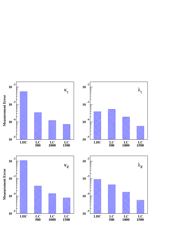
Figure 1: Expected measurement error for the real part of four different TGCs. The numbers below the “LC” labels refer to the center-of-mass energy of the linear collider in GeV. The luminosity of the LHC is assumed to be 300 fb^-1, while the luminosities of the linear colliders are assumed to be 500, 1000, and 1000 fb^-1 for $\sqrt{s}$=500, 1000, and 1500 GeV respectively.

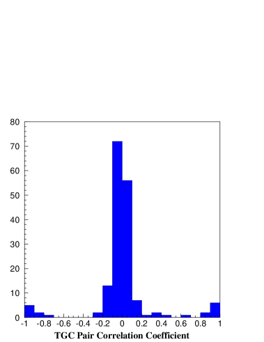
Figure 2: Histogram of correlation coefficients for all 171 pairs of TGCs when 19 different TGCs are measured using one-parameter fits at LEP2 (unpolarized beams). The 19 TGCs are made up of the real and imaginary parts of the 8 C- and P-violating couplings along with the real parts of the three CP-conserving couplings $g^{Z}_{1}$, $\kappa_{\gamma}$, $\lambda_{\gamma}$.

3 Electroweak radiative corrections to $e^{+}e^{-}\to 4$ fermions

We have seen that the experimental accuracy at a linear collider for the basic electroweak cross section measurements is expected to be at the level of $0.1-0.01\%$, requiring the inclusion of electroweak radiative corrections to the predictions for the underlying production processes such as $e^{+}e^{-}\to WW\to 4f$.

The full treatment of the processes $e^{+}e^{-}\to 4f$ at the one-loop level is of enormous complexity. Nevertheless there is ongoing work in this direction [9]. While the real bremsstrahlung contribution is known exactly, there are severe theoretical problems with the virtual order-$\alpha$ corrections. A detailed description of the status of predictions for $e^{+}e^{-}\to 4f(\gamma)$ processes can be found in [10]. A suitable approach to include order-$\alpha$ corrections to gauge-boson pair production is a double-pole approximation (DPA), keeping only those terms in an expansion about the gauge-boson resonance poles that are enhanced by two resonant gauge bosons. All present calculations of order-$\alpha$ corrections to $e^{+}e^{-}\to WW\to 4f$ rely on a DPA [11, 12, 13, 14]. Different versions of a DPA have been implemented in the Monte Carlo (MC) generators RacoonWW [12] and YFSWW3 [13]. The intrinsic DPA error is estimated to be $\alpha\Gamma_{W}/(\pi M_{W})\sim 0.5\%$ whenever the cross section is dominated by doubly resonant contributions. This is the case at LEP2 energies sufficiently above threshold. The DPA is not a valid approximation close to the $W$-pair production threshold. At higher energies diagrams without two resonant $W$ bosons become sizable, especially single $W$ production, and appropriate cuts must be applied to extract the $WW$ signal.

The theoretical uncertainty of present predictions for the total $W$-pair production cross section, $\sigma_{WW}$, is of the order of $0.5\%$ for energies between 170 GeV and 500 GeV [10], which is within the expected DPA uncertainty. This is a result of a tuned numerical comparison between the state-of-the-art MC generators RacoonWW and YFSWW3, supported by a comparison with a semi-analytical calculation [11] and a study of the intrinsic DPA ambiguity with RacoonWW [10, 12]. In the threshold region $\sigma_{WW}$ is known only to about $2\%$, since predictions are based on an improved Born approximation [10] that neglects non-universal electroweak corrections. Further improvements of the theoretical uncertainty on $\sigma_{WW}$ are anticipated only when the full order-$\alpha$ calculation becomes available. Above 500 GeV, large electroweak logarithms of Sudakov type become increasingly important and contributions of higher orders need to be taken into account.

A tuned comparison has also been performed of RacoonWW and YFSWW3 predictions for the $W$ invariant mass and the $W$ production angle distributions, as well as for several photon observables such as photon energy and production angle distributions, at 200 GeV [10, 15] and 500 GeV [15]. Taking the observed differences between the RacoonWW and YFSWW3 predictions as a guideline, a theoretical uncertainty of the order of $1\%$ can be assigned to the $W$ production angle distribution and the $W$ invariant mass distribution in the $W$ resonance region. A recent comparison of RacoonWW predictions for photon observables including leading higher-order initial-state radiation [15] with YFSWW3 predictions yields relative differences of less than $5\%$ at 200 GeV and about $10\%$ at 500 GeV. These differences might be attributed to the different treatment of visible photons in the two MC generators: in RacoonWW the real order-$\alpha$ corrections are based on the full $4f+\gamma$ matrix element, while in YFSWW3 multi-photon radiation in $W$-pair production is combined with order-$\alpha^{2}$ LL photon radiation in $W$ decays.

4 Quartic gauge boson couplings

The potential for directly probing anomalous quartic gauge boson couplings (AQGCs) via triple gauge-boson production at LEP2, at a future high-energy LC, and at hadron colliders has been investigated in [15, 16, 17, 18, 19], [15, 16, 21, 22, 23] and [18, 24, 25], respectively. The AQGCs under study arise from genuine 4- and 6-dimensional operators, i.e., they have no connection to the parametrization of the anomalous TGCs. It is conceivable that there are extensions of the SM that leave the SM TGCs unchanged but modify quartic self-interactions of the electroweak gauge bosons [21]. The possible number of operators is considerably reduced by imposing a global custodial ${\rm SU}(2)$ symmetry to protect the $\rho$ parameter from large contributions, i.e., to keep $\rho$ close to 1, and by the local ${\rm U}(1)_{{\rm QED}}$ symmetry whenever a photon is involved.

The sensitivity of triple-gauge-boson cross sections to dimension-4 operators, which only involve massive gauge bosons, has been studied for a high-energy LC and the LHC in [21, 23] and [24], respectively. Only weak constraints are expected from $WWW,WWZ,WZZ$ and $ZZZ$ productions at the LHC [24], but these processes may provide complementary information if non-zero AQGCs are found. The genuine dimension-4 AQGCs may be best probed in a multi-TeV LC. The sensitivity to the two ${\rm SU}(2)_{c}$-conserving AQGCs in the processes $e^{+}e^{-}\to 6f$ at a 1 TeV LC with a luminosity of 1000 ${\rm fb}^{-1}$ can be expected to be between $10^{-3}$ and $10^{-2}$ [23].

The following discussion is restricted to AQGCs involving at least one photon, which can be probed in $WW\gamma,ZZ\gamma,Z\gamma\gamma$ and $W\gamma\gamma$ production. The lowest-dimension operators that lead to the photonic AQGCs $a_{0}$, $a_{\rm c}$, $a_{\rm n}$, $\tilde{a}_{0}$, and $\tilde{a}_{\rm n}$ are of dimension-6 [15, 21, 22, 25] and yield anomalous contributions to the SM $WW\gamma\gamma,WWZ\gamma$ vertices, and a non-standard $ZZ\gamma\gamma$ interaction at the tree level. Most studies of AQGCs consider the separately P- and C-conserving couplings $a_{0},a_{\rm c}$ and the CP-violating coupling $a_{\rm n}$. Recently the P-violating AQGCs $\tilde{a}_{0}$, and $\tilde{a}_{\rm n}$ have also been considered [15]. More general AQGCs that have been embedded in manifestly ${\rm SU}(2)_{\rm L}\times{\rm U}(1)_{\rm Y}$ gauge invariant operators are discussed in [17, 19]. The AQGCs depend on a mass scale $\Lambda$ characterizing the scale of new physics. The choice for $\Lambda$ is arbitrary as long as no underlying model is specified which gives rise to the AQGCs. For instance, anomalous quartic interactions may be interpreted as contact interactions, which might be the manifestation of the exchange of heavy particles with a mass scale $\Lambda$.

Recently, at LEP2, the first direct bounds on the AQGCs $a_{0},a_{\rm c},a_{\rm n}$ have been imposed by investigating the total cross sections and photon energy distributions for the processes $e^{+}e^{-}\to WW\gamma,Z\gamma\gamma,Z\nu\overline{\nu}$ [20]. The results, in units of GeV^-2, are

$$-0.037<\frac{a_{0}}{\Lambda^{2}}<0.036\qquad-0.077<\frac{a_{\rm c}}{\Lambda^{2}}<0.095\qquad-0.45<\frac{a_{\rm n}}{\Lambda^{2}}<0.41\;,$$ (1)

for 95% CL intervals. These limits are expected to improve considerably as the energy increases. It has been found that a 500 GeV LC with a total integrated luminosity of 500 ${\rm fb}^{-1}$ can improve the LEP2 limits by as much as three orders of magnitude [17].

At hadron colliders the search for AQGCs is complicated by an arbitrary form factor that is introduced to suppress unitarity-violating contributions at large parton center-of-mass energies. At the LHC, however, the dependence of a measurement of AQGCs on the form-factor parametrization may be avoided by measuring energy-dependent AQGCs [24]. At Run II of the Tevatron at 2 TeV, with 2 ${\rm fb}^{-1}$, AQGC limits comparable to the LEP2 limits are expected [18, 25].

Numerical studies of AQGCs are not yet as sophisticated as the ones for TGCs. For instance, most studies of AQGCs have not yet included gauge boson decays, and MC generators for the process $e^{+}e^{-}\to 4f+\gamma$ including photon AQGCs have only recently become available [15, 19]. To illustrate the typical size of the limits that can be obtained for the AQGCs at a 500 GeV LC with 50 ${\rm fb}^{-1}$, the following $1\sigma$ bounds have been extracted from the total cross section measurement of $e^{+}e^{-}\to u\overline{d}\mu^{-}\overline{\nu}_{\mu}+\gamma$, with all bounds in units of $10^{-3}\;{\rm GeV}^{-2}$ [15]:

$$-0.12<\frac{a_{0}}{\Lambda^{2}}<0.14 -0.31<\frac{a_{\rm c}}{\Lambda^{2}}<0.16\qquad-0.82<\frac{a_{\rm n}}{\Lambda^{2}}<0.79\qquad$$

$$-0.10<\frac{\tilde{a}_{0}}{\Lambda^{2}}<0.10 -0.69<\frac{\tilde{a}_{\rm n}}{\Lambda^{2}}<0.90\;.$$ (2)

The availability of MC programs [15, 19, 23] will allow more detailed studies to be performed. For example, longitudinally polarized gauge bosons have the greatest effect on AQGCs, and gauge bosons with this polarization can be isolated through an analysis of gauge boson production and decay angles [21].

3 Strongly coupled theories

The Standard Model with a light Higgs boson provides a good fit to the electroweak data. Nevertheless, the electroweak observables depend only logarithmically on the Higgs mass, so that the effects of the light Higgs could be mimicked by new particles with masses as large as several TeV. A recent review of such scenarios is given in [26]. One can even imagine that no Higgs boson exists. In that case, the electroweak symmetry should be broken by some other interactions, and gauge boson scattering should become strong at a scale of order 1 TeV. An often discussed class of theories of this kind is called technicolor [27], which is discussed in the next subsection.

Electroweak symmetry is often assumed to be either connected to supersymmetry or driven by some strong dynamics, such as technicolor, without a Higgs boson. There is, however, a distinctive alternative where a strong interaction gives rise to bound states that include a Higgs boson. The latter could be light and weakly coupled at the electroweak scale. At sub-TeV energies these scenarios are described by a (possibly extended) Higgs sector, while the strong dynamics manifests itself only above a TeV or so.

1 Strong $WW$ scattering and technicolor

The generic idea of technicolor theories is that a new gauge interaction, which is asymptotically free, becomes strong at a scale of order 1 TeV, such that the new fermions (“technifermions”) that feel this interaction form condensates that break the electroweak symmetry. This idea is based on the observed dynamics of QCD, but arguments involving the fits to the electroweak data and the generation of quark masses suggest that the technicolor interactions should be described by a strongly coupled gauge theory that has a different behavior from QCD (see, e.g., [28]).

A generic prediction of technicolor theories is that there is a vector resonance with mass below about 2 TeV which unitarizes the $WW$ scattering cross section. In what follows we will concentrate on the capability of a linear $e^{+}e^{-}$ collider of studying $WW$ scattering, but first we briefly mention other potential signatures associated with various technicolor models. The chiral symmetry of the technifermions may be large enough that its dynamical breaking leads to pseudo-Goldstone bosons, which are pseudoscalar bound states that can be light enough to be produced at a linear $e^{+}e^{-}$ collider (for a recent study, see [29]). The large top-quark mass typically requires a special dynamics associated with the third generation. A thoroughly studied model along these lines is called Topcolor Assisted Technicolor [30], and leads to a rich phenomenology. This model predicts the existence of spinless bound states with large couplings to the top quark, called top-pions and top-Higgs, which may be studied at a linear $e^{+}e^{-}$ collider [31].

Strong $W^{+}W^{-}$ scattering is an essential test not only of technicolor theories, but in fact of any model that does not include a Higgs boson with large couplings to gauge boson pairs. It can be studied at a linear collider with the reactions $e^{+}e^{-}\rightarrow\nu\overline{\nu}W^{+}W^{-}$, $\nu\overline{\nu}ZZ$, $\nu\overline{\nu}t\overline{t}$, and $W^{+}W^{-}$ [32]. The final states $\nu\overline{\nu}W^{+}W^{-}$, $\nu\overline{\nu}ZZ$ are used to study the I=J=0 channel in $W^{+}W^{-}$ scattering, while the final state $W^{+}W^{-}$ is best suited for studying the I=J=1 channel. The $\nu\overline{\nu}t\overline{t}$ final state can be used to investigate strong electroweak symmetry breaking in the fermion sector through the process $W^{+}W^{-}\rightarrow t\overline{t}$.

The first step in studying strong $W^{+}W^{-}$ scattering is to separate the scattering of a pair of longitudinally polarized $W$’s, denoted by $W_{\rm L}W_{\rm L}$, from transversely polarized $W$’s, and from background such as $e^{+}e^{-}\rightarrow e^{+}e^{-}W^{+}W^{-}$ and $e^{-}\overline{\nu}W^{+}Z$. Studies have shown that simple cuts can be used to achieve this separation in $e^{+}e^{-}\rightarrow\nu\overline{\nu}W^{+}W^{-}$, $\nu\overline{\nu}ZZ$ at $\sqrt{s}=1000$ GeV, and that the signals are comparable to those obtained at the LHC [33]. Furthermore, by analyzing the gauge boson production and decay angles it is possible to use these reactions to measure chiral Lagrangian parameters with an accuracy greater than that which can be achieved at the LHC [34].

The reaction $e^{+}e^{-}\rightarrow\nu\overline{\nu}t\overline{t}$ provides unique access to $W^{+}W^{-}\rightarrow t\overline{t}$, since this process is overwhelmed by the background $gg\rightarrow t\overline{t}$ at the LHC. Techniques similar to those employed to isolate $W_{\rm L}W_{\rm L}\rightarrow W^{+}W^{-},ZZ$ can be used to measure the enhancement in $W_{\rm L}W_{\rm L}\rightarrow t\overline{t}$ production [35]. Even in the absence of a resonance it will be possible to establish a clear signal. The ratio $S/\sqrt{B}$ is expected to be 12 for a linear collider with $\sqrt{s}=1$ TeV and 1000 fb^-1 and 80%/0% electron/positron beam polarization, increasing to 28 for the same data sample at 1500 GeV.

There are two approaches to studying strong $W^{+}W^{-}$ scattering with the process $e^{+}e^{-}\rightarrow W^{+}W^{-}$. The first approach was discussed in Section 2: a strongly coupled gauge boson sector induces anomalous TGCs that could be measured in $e^{+}e^{-}\rightarrow W^{+}W^{-}$. The precision of $4\times 10^{-4}$ for the TGCs $\kappa_{\gamma}$ and $\kappa_{Z}$ at $\sqrt{s}=500$ GeV can be interpreted as a precision of $0.26$ for the chiral Lagrangian parameters $L_{9L}$ and $L_{9R}$. Assuming naive dimensional analysis [36], such a measurement would provide a $8\sigma$ ($5\sigma$) signal for $L_{9L}$ and $L_{9R}$ if the strong symmetry breaking energy scale were 3 TeV (4 TeV). The only drawback to this approach is that the detection of anomalous TGCs does not by itself provide unambiguous proof of strong electroweak symmetry breaking.

The second approach involves an effect unique to strong $W^{+}W^{-}$ scattering. When $W^{+}W^{-}$ scattering becomes strong the amplitude for $e^{+}e^{-}\rightarrow W_{\rm L}W_{\rm L}$ develops a complex form factor $F_{T}$ in analogy with the pion form factor in $e^{+}e^{-}\rightarrow\pi^{+}\pi^{-}$ [37]. To evaluate the size of this effect the following expression for $F_{T}$ has been suggested:

$$F_{T}=\exp\left[{1\over\pi}\int_{0}^{\infty}ds^{\prime}\delta(s^{\prime},M_{\rho},\Gamma_{\rho})\left\{{1\over s^{\prime}-s-i\epsilon}-{1\over s^{\prime}}\right\}\right]$$

where

$$\delta(s,M_{\rho},\Gamma_{\rho})={1\over 96\pi}{s\over v^{2}}+{3\pi\over 8}\left[\ \tanh({s-M_{\rho}^{2}\over M_{\rho}\Gamma_{\rho}})+1\right]\ .$$

Here $M_{\rho},\Gamma_{\rho}$ are the mass and width, respectively, of a vector resonance in $W_{\rm L}W_{\rm L}$ scattering. The term

$$\delta(s)={1\over 96\pi}{s\over v^{2}}$$

is the Low Energy Theorem (LET) amplitude for $W_{\rm L}W_{\rm L}$ scattering at energies below a resonance. Below the resonance, the real part of $F_{T}$ is proportional to $L_{9L}+L_{9R}$ and can therefore be interpreted as a TGC. The imaginary part, however, is a distinct new effect.

The real and imaginary parts of $F_{T}$ are measured [38] in the same manner as the TGCs. The $W^{+}W^{-}$ production and decay angles are analyzed, and an electron beam polarization of 80% is assumed. In contrast to TGCs, the analysis of $F_{T}$ seems to benefit from even small amounts of jet flavor tagging. We therefore assume that charm jets can be tagged with a purity/efficiency of 100/33%. These purity/efficiency numbers are based on research [39] that indicates that it may be possible to tag charm jets with a purity/efficiency as high as 100/65%, given that $b$-jet contamination is not a significant factor in $W^{+}W^{-}$ pair production and decay.

The expected 95% confidence level limits for $F_{T}$ for $\sqrt{s}=500$ GeV and a luminosity of 500 fb^-1 are shown in Fig. 3, along with the predicted values of $F_{T}$ for various masses $M_{\rho}$ of a vector resonance in $W_{\rm L}W_{\rm L}$ scattering. The masses and widths of the vector resonances are chosen to coincide with those used in the ATLAS TDR [8]. The technipion form factor $F_{T}$ affects only the amplitude for $e^{+}e^{-}\rightarrow W_{\rm L}W_{\rm L}$, whereas TGCs affect all amplitudes. Through the use of electron beam polarization and the rich angular information in $W^{+}W^{-}$ production and decay, it will be possible to disentangle anomalous values of $F_{T}$ from other anomalous TGC values and to deduce the mass of a strong vector resonance well below threshold, as suggested by Fig. 3.

Figure 3: 95% C.L. contour for $F_{T}$ for $\sqrt{s}=500$ GeV and 500 fb^-1. Values of $F_{T}$ for various masses $M_{\rho}$ of a vector resonance in $W_{\rm L}W_{\rm L}$ scattering are also shown. The $F_{T}$ point “LET” refers to the case where no vector resonance exists at any mass in strong $W_{\rm L}W_{\rm L}$ scattering.

The signal significances obtained by combining the results for $e^{+}e^{-}\rightarrow\nu\overline{\nu}W^{+}W^{-}$, $\nu\overline{\nu}ZZ$ [33] with the $F_{T}$ analysis of $W^{+}W^{-}$ [38] are displayed in Fig. 4 along with the results expected from the LHC [8]. The LHC signal is a mass bump in $W^{+}W^{-}$; the LC signal is less direct. Nevertheless, the signals at the LC are strong, particularly in $e^{+}e^{-}\to W^{+}W^{-}$, where the technirho effect gives a large enhancement of a very well-understood Standard Model process. Since the technipion form factor includes an integral over the technirho resonance region, the linear collider signal significance is relatively insensitive to the technirho width. (The real part of $F_{T}$ remains fixed as the width is varied, while the imaginary part grows as the width grows.) The LHC signal significance will drop as the technirho width increases. The large linear collider signals can be utilized to study a vector resonance in detail; for example, the evolution of $F_{T}$ with $\hat{s}$ can be determined by measuring the initial-state radiation in $e^{+}e^{-}\rightarrow W^{+}W^{-}$.

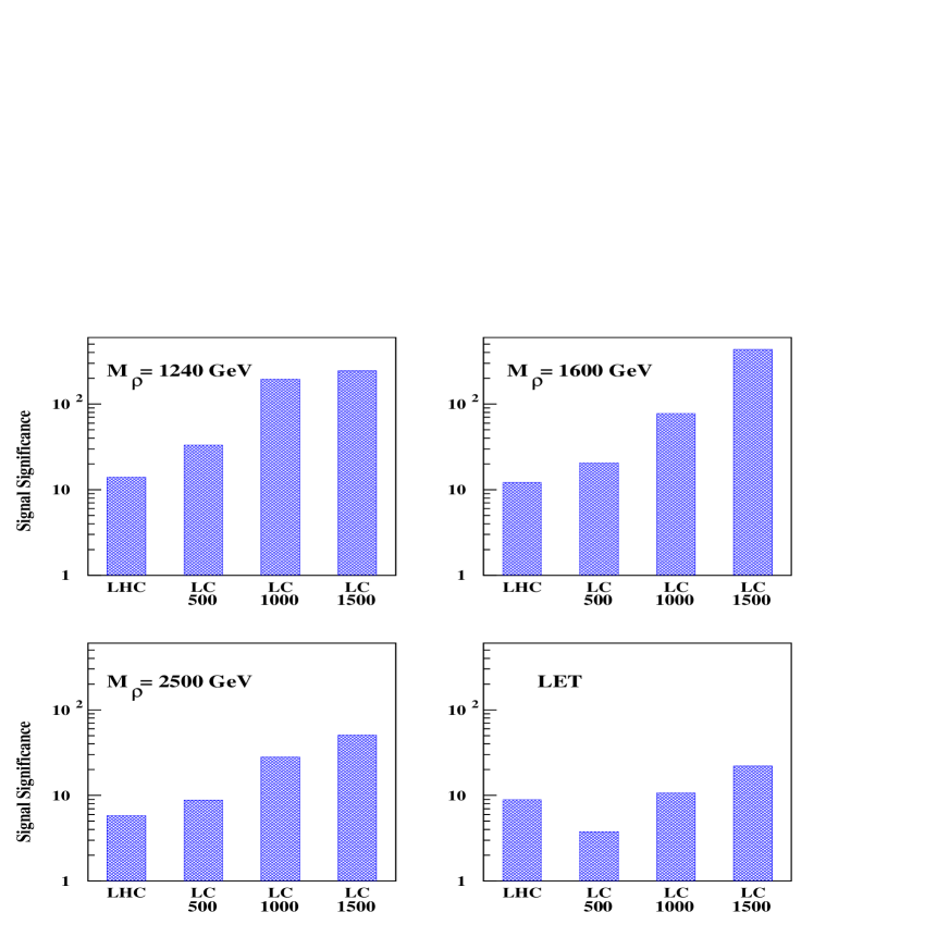
Figure 4: Direct strong symmetry breaking signal significance in $\sigma$’s for various masses $M_{\rho}$ of a vector resonance in $W_{\rm L}W_{\rm L}$ scattering. In the first three plots the signal at the LHC is a bump in the $WW$ cross section; in the LET plot, the LHC signal is an enhancement over the SM cross section. The various LC signals are for enhancements of the amplitude for pair production of longitudinally polarized $W$ bosons. The numbers below the “LC” labels refer to the center-of-mass energy of the linear collider in GeV. The luminosity of the LHC is assumed to be 300 fb^-1, while the luminosities of the linear colliders are assumed to be 500, 1000, and 1000 fb^-1 for $\sqrt{s}$=500, 1000, and 1500 GeV respectively. The lower right hand plot “LET” refers to the case where no vector resonance exists at any mass in strong $W_{\rm L}W_{\rm L}$ scattering.

Only when the vector resonance disappears altogether (the LET case in the lower right-hand panel in Fig. 4 ) does the direct strong symmetry breaking signal from the $\sqrt{s}=500$ GeV linear collider drop below the LHC signal. At higher $e^{+}e^{-}$ center-of-mass energies the linear collider signal exceeds the LHC signal.

2 Composite Higgs models

The good fit of the Standard Model to the electroweak data suggests that the new physics has a decoupling limit in which the new particles carrying $SU(2)_{W}\times U(1)_{Y}$ charges can be much heavier than the electroweak scale without affecting the Standard Model. This is the reason why the Minimal Supersymmetric Standard Model is viable: all the superpartners and the states associated with a second Higgs doublet can be taken to be heavier than the electroweak scale, leaving a low-energy theory given by the Standard Model. At the same time, it is hard to construct viable technicolor models because they do not have a decoupling limit: the new fermions that condense and give the $W$ and $Z$ masses are chiral, i.e., their masses break the electroweak symmetry.

There is a class of models of electroweak symmetry breaking that have a decoupling limit given by the Standard Model, so they are phenomenologically viable, and yet the Higgs field arises as a bound state due to some strong interactions. An example of such a composite Higgs model is the Top Quark Seesaw Theory, in which a Higgs field appears as a bound state of the top quark with a new heavy quark. This has proven phenomenologically viable and free of excessive fine-tuning [40]. Furthermore, the top quark is naturally the heaviest Standard Model fermion in this framework, because it participates directly in the breaking of the electroweak symmetry.

The interaction responsible for binding the Higgs field is provided by a spontaneously broken gauge symmetry, such as topcolor [41], or some flavor or family symmetry [42]. Such an interaction is asymptotically free, allowing for a solution to the hierarchy problem. At the same time the interaction is non-confining, and therefore has a very different behavior from the technicolor interaction discussed in the first part of this section.

Typically, in the top quark seesaw theory, the Higgs boson is heavy, with a mass of order 500 GeV [43]. However, the effective theory below the compositeness scale may include an extended Higgs sector, in which case the mixing between the CP-even scalars could bring the mass of the Standard Model-like Higgs boson down to the current LEP limit [40, 44]. One interesting possibility in this context is that there is a light Higgs boson with nearly standard couplings to fermions and gauge bosons, but whose decay modes are completely non-standard. This happens whenever a CP-odd scalar has a mass less than half the Higgs mass and the coupling of the Higgs to a pair of CP-odd scalars is not suppressed. The Higgs boson decays in this case into a pair of CP-odd scalars, each of them subsequently decaying into a pair of Standard Model particles with model-dependent branching fractions [45]. If the Higgs boson has Standard Model branching fractions, then the capability of an $e^{+}e^{-}$ linear collider depends on $M_{H}$, as discussed in [46]. On the other hand, if the Higgs boson has non-standard decays, an $e^{+}e^{-}$ collider may prove very useful in disentangling the composite nature of the Higgs boson, by measuring its width and branching fractions.

The heavy-quark constituent of the Higgs has a mass of a few TeV, and the gauge bosons associated with the strong interactions that bind the Higgs are expected to be even heavier. Above the compositeness scale there must be some additional physics that leads to the spontaneous breaking of the gauge symmetry responsible for binding the Higgs. This may involve new gauge dynamics [47], or fundamental scalars and supersymmetry. For studying these interesting strongly interacting particles, the $e^{+}e^{-}$ collider should operate at the highest energy achievable.

Other models of Higgs compositeness have been proposed recently [48], and more are likely to be constructed in the future. Another framework in which a composite Higgs boson arises from a strong interaction is provided by extra spatial dimensions accessible to the Standard Model particles; this is discussed in Section 6.

4 Contact interactions and compositeness

There is a strong historical basis for the consideration of composite models that is currently mirrored in the proliferation of fundamental particles. If the fermions have substructure, then their constituents are bound by a confining force at the mass scale $\Lambda$, which characterizes the radius of the bound states. At energies above $\Lambda$, the composite nature of fermions would be revealed by the break-up of the bound states in hard scattering processes. At lower energies, deviations from the Standard Model may be observed via form factors or residual effective interactions induced by the binding force. These composite remnants are usually parameterized by the introduction of contact terms in the low-energy Lagrangian. More generally, four-fermion contact interactions represent a useful parametrization of many types of new physics originating at high energy scales, and specific cases will be discussed throughout this chapter.

The lowest-order four-fermion contact terms are of dimension 6. A general helicity-conserving, flavor-diagonal, Standard Model-invariant parameterization can be written as [49]

$${\cal L}={g^{2}_{\rm eff}\eta\over\Lambda^{2}}\left(\overline{q}\gamma^{\mu}q+{\cal F}_{\ell}\overline{\ell}\gamma^{\mu}\ell\right)_{L/R}\left(\overline{q}\gamma_{\mu}q+{\cal F}_{\ell}\overline{\ell}\gamma_{\mu}\ell\right)_{L/R}\,,$$ (3)

where the generation and color indices have been suppressed, $\eta=\pm 1$, and ${\cal F}_{\ell}$ is inserted to allow for different quark and lepton couplings but is anticipated to be ${\cal O}(1)$. Since the binding force is expected to be strong when $Q^{2}$ approaches $\Lambda^{2}$, it is conventional to define $g^{2}_{\rm eff}=4\pi$.

Interference between the contact terms and the usual gauge interactions can lead to observable deviations from Standard Model predictions at energies lower than $\Lambda$. Currents limits from various processes at the Tevatron and LEP II place $\Lambda$ above the few-TeV range. At the LHC [8], $\Lambda_{\ell q}$ terms can be probed to $\sim 20-30$ TeV for integrated luminosities of $10-100$ fb^-1, while the $\Lambda_{qq}$ case is more problematic because of uncertainties in the parton distributions and the extrapolation of the calorimeter energy calibration to very high values of the jet $p_{T}$.

At a LC, the use of polarized beams, combined with angular distributions, allows for a clear determination of the helicity of the contact term. An examination of contact effects in $e^{+}e^{-}\to f\overline{f}$, where $f=\mu\,,c\,,b$ was performed for LC energies in [50]. This study concentrated on tagged final states, since contact effects are diluted when all quark flavors are summed because of cancellations between the up- and down-type quarks. Here, both polarized and unpolarized angular distributions were examined with tagging efficiencies of 60% and 35% for $b$- and $c$-quarks, respectively, and the detector acceptance was taken to be $|\cos\theta|<0.985$. The resulting 95% CL sensitivity for ${\cal L}=500$ fb^-1 to $\Lambda$ from the polarized distributions with 90% electron beam polarization is listed in Table 3.

	$\Lambda_{LL}$	$\Lambda_{LR}$	$\Lambda_{RL}$	$\Lambda_{RR}$
$\sqrt{s}=0.5$ TeV
$e^{-}_{L}e^{+}\to\mu^{+}\mu^{-}$	57	52	18	18
$e^{-}_{R}e^{+}\to\mu^{+}\mu^{-}$	20	18	52	55
$e^{-}_{L}e^{+}\to c\overline{c}$	59	50	9	15
$e^{-}_{R}e^{+}\to c\overline{c}$	21	20	43	57
$e^{-}_{L}e^{+}\to b\overline{b}$	68	53	9	16
$e^{-}_{R}e^{+}\to b\overline{b}$	30	21	59	59
$\sqrt{s}=1.0$ TeV
$e^{-}_{L}e^{+}\to\mu^{+}\mu^{-}$	79	72	25	26
$e^{-}_{R}e^{+}\to\mu^{+}\mu^{-}$	28	25	73	78
$e^{-}_{L}e^{+}\to c\overline{c}$	82	72	12	21
$e^{-}_{R}e^{+}\to c\overline{c}$	30	28	62	78
$e^{-}_{L}e^{+}\to b\overline{b}$	94	77	14	23
$e^{-}_{R}e^{+}\to b\overline{b}$	43	30	82	84

Table 3: 95% CL search reach in TeV for contact interaction scales with various helicities.

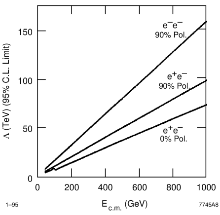
Figure 5: The 95% confidence level limits for the compositeness scale $\Lambda^{+}_{\rm LL}$ from Møller and Bhabha scattering as a function of the $e^{-}e^{-}\,$or $e^{+}e^{-}$ center-of-mass energy. The luminosity is given by ${\cal L}=680\ {\rm pb}^{-1}\cdot s/M_{Z}^{2}$. The polarization of the electron beam(s) is indicated in the figure.

Compositeness limits for $\Lambda^{+}_{\rm LL}$ from Møller and Bhabha scattering [51] are summarized in Fig. 5. For equal luminosities the limits from Møller scattering are significantly better than those from Bhabha scattering. This is due not only to the polarization of both beams, but also to the Møller/Bhabha crossing relation in the central region of the detector. Limits on $\Lambda^{+}_{\rm LL}$ for different energies and luminosities can be calculated under the assumption that the compositeness limit scales as ${\cal{L}}^{1/4}s^{1/2}$.

5 New particles in extended gauge sectors and GUTs

1 Extended gauge sectors

New gauge bosons are a feature of many extensions of the Standard Model. They arise naturally in grand unified theories, such as $SO(10)$ and $E_{6}$, where the GUT group gives rise to extra $U(1)$ or $SU(2)$ subgroups after decomposition. There are also numerous non-unified extensions, such as the Left-Right Symmetric model and Topcolor. More recently, there has been renewed interest in Kaluza-Klein excitations of the SM gauge bosons, which are realized in theories of extra space dimensions at semi-macroscopic scales. All of these extensions of the SM predict the existence of new gauge bosons, generically denoted as $Z^{\prime}$ or $W^{\prime}$. The search for extra gauge bosons thus provides a common coin in the quest for new physics at high-energy colliders. Here, we concentrate on the most recent developments on the subject, and refer the interested to recent reviews [52].

$Z^{\prime}$ discovery limits and identification

The signal for the existence of a new neutral gauge boson at linear collider energies arises through the indirect effects of $s$-channel $Z^{\prime}$ exchange. Through its interference with the SM $\gamma$ and $Z$ exchange in $e^{+}e^{-}\to f\overline{f}$, significant deviations from SM predictions can occur even when $M_{Z^{\prime}}$ is much larger than $\sqrt{s}$. This sensitivity to the $Z^{\prime}$ nicely complements the ability of the LHC to discover a $Z^{\prime}$ as a resonance in lepton pair production. The combination of many LC observables such as the cross sections for $f\overline{f}$ final states, forward-backward asymmetries, $A_{FB}^{f}$, and left-right asymmetries, $A_{LR}^{f}$, where $f=\mu$, $\tau$, $c$, $b$, and light quarks, can fill in the detailed picture of the $Z^{\prime}$ couplings.

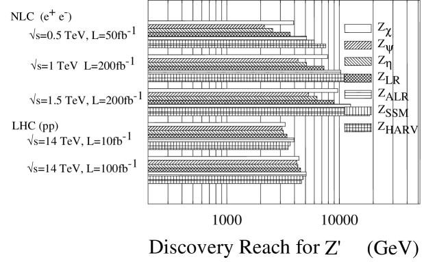
Figure 6: $95\%$ CL search limits for extra neutral gauge bosons, for various models, at high-energy linear colliders, by observation of corrections to $e^{+}e^{-}\to f\overline{f}$ processes, and at the LHC, by observation of a peak in dilepton pairs.

The combined sensitivity of the LC measurements for various $Z^{\prime}$ models is shown in Fig. 6 [52]. We see that if a $Z^{\prime}$ is detected at the LHC, precision measurements at the LC could be used to measure its properties and determine the underlying theory. Figure 7 displays the resolving power between $Z^{\prime}$ models assuming that the mass of the $Z^{\prime}$ was measured previously at the LHC. This study only considers leptonic final states and assumes lepton universality. If $M_{Z^{\prime}}$ were beyond the LHC discovery reach or if the $Z^{\prime}$ does not couple to quarks then no prior knowledge of it would be obtained before the LC turns on. However, in this case, the LC can still yield some information on the $Z^{\prime}$ couplings and mass. Instead of extracting $Z^{\prime}$ couplings directly, “normalized” couplings, defined by

$$a_{f}^{N}=a_{f}^{\prime}\sqrt{{s\over{M_{Z^{\prime}}^{2}-s}}};\quad v_{f}^{N}=v_{f}^{\prime}\sqrt{{s\over{M_{Z^{\prime}}^{2}-s}}}$$ (4)

could be measured. For a demonstration of this case, the diagnostic power of a 1 TeV LC for a $Z^{\prime}$ with couplings of the $E_{6}$ model $\chi$ and mass $M_{Z^{\prime}}=5$ TeV is displayed in Fig. 7 for $f=\ell$. An additional determination of the $Z^{\prime}$ mass and couplings could be performed [52] in this case from cross section and asymmetry measurements at several different values of $\sqrt{s}$.

A recent study of the process $e^{+}e^{-}\to\nu\overline{\nu}\gamma$ has demonstrated that the process can also be used to obtain information on $Z^{\prime}-\nu\overline{\nu}$ couplings [53].

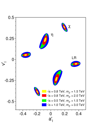
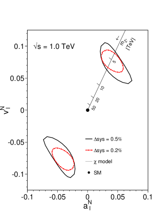
Figure 7: Left Panel: Resolution power (95% C.L.) for different $M_{Z^{\prime}_{\chi}}$ based on measurements of leptonic observables at $\sqrt{s}=1$  TeV with a luminosity of $L_{\rm int}=1\;$ab^-1 [56]. Right Panel: Resolution power (95% C.L.) for different $M_{Z^{\prime}}$ based on measurements of leptonic observables at $\sqrt{s}=500$ GeV, 800 GeV, 1 TeV with a luminosity of $L_{\rm int}=1\;$ab^-1. The leptonic couplings of the $Z^{\prime}$ correspond to the $\chi$, $\eta$, or $LR$ model [56].

$W^{\prime}$  discovery limits and identification

While considerable effort has been devoted to the study of $Z^{\prime}$ bosons at $e^{+}e^{-}$ colliders, a corresponding endeavor for the $W^{\prime}$ sector has only recently been undertaken. A preliminary investigation [54] of the sensitivity of $e^{+}e^{-}\to\nu\overline{\nu}\gamma$ to $W^{\prime}$ bosons was performed at Snowmass 1996, and more detailed examinations [53, 55] have recently been performed. The models with extra $SU(2)$ factors considered in these studies are the Left-Right symmetric model (LRM) based on the gauge group $SU(2)_{L}\times SU(2)_{R}\times U(1)_{B-L}$, the Un-Unified model (UUM) based on $SU(2)_{q}\times SU(2)_{l}\times U(1)_{Y}$ where the quarks and leptons each transform under their own $SU(2)$, a Third Family Model (3FM) based on the group $SU(2)_{h}\times SU(2)_{l}\times U(1)_{Y}$ where the quarks and leptons of the third (heavy) family transform under a separate group, and the KK model which contains the Kaluza-Klein excitations of the SM gauge bosons that are a possible consequence of theories with large extra dimensions.

In the process $e^{+}e^{-}\rightarrow\nu\overline{\nu}\gamma$, both charged and neutral extra gauge bosons can contribute. In the analysis of [53], the photon energy and angle with respect to the beam axis are restricted to $E_{\gamma}\geq 10$ GeV and $10^{\circ}\leq\theta_{\gamma}\leq 170^{\circ}$, to take into account detector acceptance. The most serious background, radiative Bhabha scattering in which the scattered $e^{+}$ and $e^{-}$ go undetected down the beam pipe, is suppressed by restricting the photon’s transverse momentum to $p_{T}^{\gamma}>\sqrt{s}\sin\theta_{\gamma}\sin\theta_{v}/(\sin\theta_{\gamma}+\sin\theta_{v})$, where $\theta_{v}$ is the minimum angle at which the veto detectors may observe electrons or positrons; here, $\theta_{v}=25$ mrad. The observable $d\sigma/dE_{\gamma}$ was found to provide the most statistically significant search reach. The $95\%$ CL reach is displayed graphically in Fig. 8 and in Table 4, which shows the degradation when a 2% systematic error is added in quadrature with the statistical error. The corresponding $W^{\prime}$ search reach at the LHC is in the range 5–6 TeV [52].

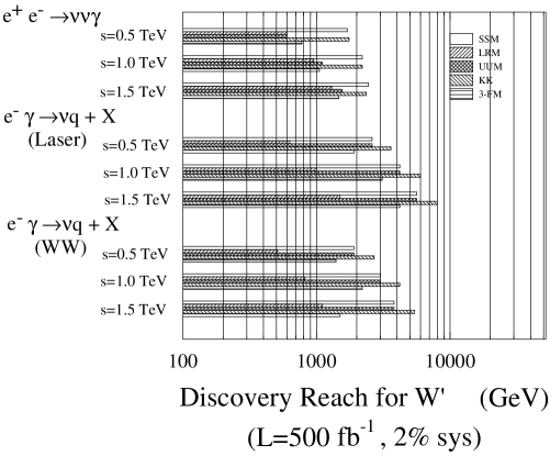
Figure 8: 95% CL search limits for $W^{\prime}$ bosons at the LC.

The 95% CL constraints that can be placed on the right- and left-handed couplings of a $W^{\prime}$ to fermions, assuming that the $W^{\prime}$ has Standard Model-like couplings, and that there is no corresponding $Z^{\prime}$ contribution to $e^{+}e^{-}\to\nu\overline{\nu}\gamma$, are shown in Fig. 9. Here, the total cross section $\sigma$ and the left-right asymmetry $A_{LR}$ are used as observables, with the systematic errors for $\sigma(A_{LR})$ taken as 2%(1%) and 80% electron and 60% positron polarization are assumed. The axes in this figure correspond to couplings normalized as $L_{f}(W)=C_{L}^{W^{\prime}}g/(2\sqrt{2})$ and similarly for $R_{f}(W)$. It is found that 2% systematic errors dominate the coupling determination. In addition, we note that the $W^{\prime}$ couplings can only be constrained up to a two-fold ambiguity, which could be resolved by reactions in which the $W^{\prime}$ couples to a triple gauge vertex.

Additional sensitivity to the existence of a $W^{\prime}$ can be gained from $e\gamma\rightarrow\nu q+X$ [55]. This process receives contributions only from charged and not from neutral gauge bosons. The $W^{\prime}$ contribution can be isolated by imposing a kinematic cut requiring either the $q$ or $\overline{q}$ to be collinear to the beam axis. In order to take into account detector acceptance, the angle $\theta_{q}$ of the detected quark relative to the beam axis is restricted to $10^{\circ}\leq\theta_{q}\leq 170^{\circ}$. The kinematic variable that is most sensitive to a $W^{\prime}$ is the $p_{T_{q}}$ distribution. The quark’s transverse momentum relative to the beam is restricted to $p_{T}^{q}>40(75)$ GeV for $\sqrt{s}=0.5(1.0)$  TeV, to suppress various Standard Model backgrounds. Figure 9 and Table 4 show the resulting 95% CL constraints on the $W^{\prime}$ fermionic couplings for the case of backscattered laser photons. As seen above, the assumed systematic error of 2% again dominates the statistical error, thus eliminating the potential gain from high luminosities. $W^{\prime}$ coupling determination from backscattered laser photons are considerably better than those from Weizsäcker-Williams photons or from $e^{+}e^{-}$ collisions. Polarized beams give only a minor improvement to these results after the inclusion of systematic errors.

     

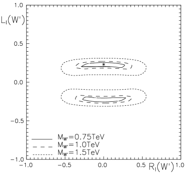
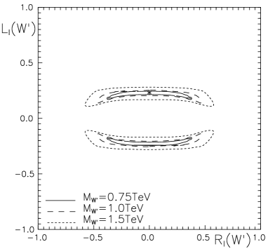
Figure 9: Left Panel: 95% CL constraints from $e^{+}e^{-}\to\nu\overline{\nu}\gamma$ on couplings of the SSM $W^{\prime}$ indicated by a star for $\sqrt{s}=0.5$  TeV and $L_{\rm int}=1000$  fb^-1 with a systematic error of 0.5% (0.25%) for $\sigma(A_{LR})$ for different $W^{\prime}$ masses. Right Panel: 95% C.L. constraints from $e\gamma\to\overline{\nu}q+X$ on couplings of the SSM $W^{\prime}$ for $\sqrt{s}=0.5$  TeV and $L_{\rm int}=1000\ {\rm fb}^{-1}$ with a 2% systematic error for different $W^{\prime}$ masses.

If a $W^{\prime}$ were discovered elsewhere, measurements of its couplings in both $e^{+}e^{-}\to\nu\overline{\nu}\gamma$ and $e\gamma\to\nu q+X$ could provide valuable information regarding the underlying model, with the latter process serving to isolate the $W^{\prime}$ couplings from those of the $Z^{\prime}$.

	$\sqrt{s}=0.5$ TeV, $L_{\rm int}=500$ fb-1				$\sqrt{s}=1$ TeV, $L_{\rm int}=500$ fb-1
	$e^{+}e^{-}\rightarrow\nu\overline{\nu}\gamma$		$e\gamma\rightarrow\nu q+X$		$e^{+}e^{-}\rightarrow\nu\overline{\nu}\gamma$		$e\gamma\rightarrow\nu q+X$
Model	no syst.	syst.	no syst	syst.	no syst.	syst.	no syst.	syst.
SSM $W^{\prime}$	4.3	1.7	4.1	2.6	5.3	2.2	5.8	4.2
LRM	1.2	0.6	0.8	0.6	1.6	1.1	1.2	1.1
UUM	2.1	0.6	4.1	2.6	2.5	1.1	5.8	4.2
KK	4.6	1.8	5.7	3.6	5.8	2.2	8.3	6.0
3FM	2.3	0.8	3.1	1.9	2.7	1.1	4.4	3.1

Table 4: 95% CL search limits for $W^{\prime}$ bosons, in TeV, for various reactions.

2 Leptoquarks

Leptoquarks are natural in theories that relate leptons and quarks at a more fundamental level. These spin-0 or -1 particles carry both baryon and lepton number and are color triplets under SU(3)_C. They can be present at the electroweak scale in models where baryon and lepton number are separately conserved, thus avoiding conflicts with rapid proton decay. Their remaining properties depend on the model in which they appear, and would need to be determined in order to ascertain the framework of the underlying theory. Given the structure of the Standard Model fermions, there are 14 different possible types of leptoquarks; their classification can be found in [57]. Their fermionic couplings proceed through a Yukawa interaction of unknown strength, while their gauge couplings are specified for a particular leptoquark. Low-energy data place tight constraints on intergenerational leptoquark Yukawa couplings and also require that these couplings be chiral. A summary of the current state of experimental searches for leptoquarks is given in [58].

At a linear collider, leptoquarks may be produced in pairs or as single particles, while virtual leptoquark exchange may be present in $e^{+}e^{-}\to$ hadrons. Pair production receives a $t$-channel quark-exchange contribution whose magnitude depends on the size of the Yukawa coupling. This only competes with the usual $s$-channel exchange, which depends on the leptoquark’s gauge couplings, if the Yukawa coupling is of order electromagnetic strength. The possible signatures are $e^{+}e^{-}$, $e^{\pm}$ plus missing $E_{T}$, or missing $E_{T}$ alone, combined with two jets. The observation is straightforward essentially up to the kinematic limit. A thorough study of the background and resulting search reach for each type of leptoquark can be found in [59]. Single leptoquark production is most easily studied in terms of the quark content of the photon [60]. In this case a lepton fuses with a quark from a Weiszäcker-Williams photon (in $e^{+}e^{-}$ mode) or a laser-backscattered photon (in $e\gamma$ mode) to produce a leptoquark. The cross section is a convolution of the parton-level process with distribution functions for the photon in the electron and the quark in the photon, and is directly proportional to the $eqLQ$ Yukawa coupling. The kinematic advantage of single production is lost if the Yukawa coupling is too small. For Yukawa couplings of electromagnetic strength, leptoquarks with mass up to about 90% of $\sqrt{s}$ can be discovered at a LC [60]. If the Yukawa couplings are sizable enough, then virtual leptoquark exchange [61] will lead to observable deviations in the hadronic production cross section for leptoquark masses in excess of $\sqrt{s}$. A summary of the search reach from these three processes is shown in Fig. 10 from [59] in the leptoquark mass-coupling plane. In comparison, leptoquarks are produced strongly at the LHC, with search reaches in the 1.5 TeV range [62] independent of the Yukawa couplings.

The strength of the LC is in the determination of the leptoquark’s electroweak quantum numbers and the strength of its Yukawa couplings once it is discovered. Together, the production rate and polarized left-right asymmetry can completely determine the leptoquark’s electroweak properties and identify its type [63] in both the pair and single production channels, up to the kinematic limit. In addition, the Yukawa coupling strength can be measured via the forward-backward asymmetry in leptoquark pair production (which is non-vanishing for significant Yukawa couplings), deviations in the hadronic cross sections, and the comparison of pair and single production rates.

Figure 10: Leptoquark search limits at a LC from the three processes discussed in the text. The Yukawa coupling is scaled to $e$. The pair- and single-production reaches are shown for $\sqrt{s}=1$ TeV, while the indirect reach is displayed for $\sqrt{s}=0.5$ and 1 TeV.

3 Exotic fermions

Fermions beyond the ordinary Standard Model content arise in many extensions of the Standard Model, notably in grand unified theories. They are referred to as exotic fermions if they do not have the usual SU(2)${}_{L}\times$U(1)_Y quantum numbers. For a review, we refer the reader to [64]. Examples of new fermions are the following: ($i$) The sequential repetition of a Standard Model generation (of course, in this case the fermions maintain their usual SU(2)${}_{L}\times$U(1)_Y assignments). ($ii$) Mirror fermions, which have chiral properties opposite to those of their Standard Model counterparts [65]. The restoration of left-right symmetry is a motivating factor for this possibility. ($iii$) Vector-like fermions that arise when a particular weak isospin representation is present for both left and right handed components. For instance, in E₆ grand unified theories, with each fermion generation in the representation of dimension 27, there are two additional isodoublets of leptons, one sequential (left-handed) and one mirror (right-handed). This sort of additional content is referred to as a vector doublet model (VDM) [66], whereas the addition of weak isosinglets in both chiralities is referred to as a vector singlet model (VSM) [67].

Exotic fermions can mix with the Standard Model fermions; in principle, the mixing pattern may be complicated and is model-independent. One simplifying factor is that intergenerational mixing is severely limited by the constraints on flavor-changing neutral currents, as such mixing is induced at the tree level [66]. Thus most analyses neglect intergenerational mixing. Global fits of low-energy electroweak data and the high-precision measurements of the $Z$ properties provide upper limits for the remaining mixing angles of the order of $\sin^{2}\theta_{\rm mix}\leq 10^{-2}-10^{-3}$ [68].

Exotic fermions may be produced in $e^{+}e^{-}$ collisions either in pairs or singly in association with their Standard Model partners as a result of mixing. The cross section for pair production of exotic quarks via gluon fusion and the Drell-Yan process at the LHC is large enough that the reach of the LC is unlikely to be competitive [69]. On the other hand, the backgrounds to exotic lepton production are large in $pp$ collisions, with production in $e^{+}e^{-}$ collisions providing a promising alternative. Generally, the search reach for exotic leptons is up to the kinematic limit of the $e^{+}e^{-}$ machine, for allowed mixings [70]. The experimental signature requires knowledge of the $L^{\pm}$ decay mode, which is model-dependent and also depends on the mass difference of the charged and neutral exotic leptons. Studies indicate that the signals for exotic lepton production are clear and easy to separate from Standard Model backgrounds [64, 70, 71], and that the use of polarized beams is important in determining the electroweak quantum numbers [71].

Almeida et al. have recently presented a detailed study of neutral heavy lepton production at high-energy $e^{+}e^{-}$ colliders [72]. They find single heavy neutrino production to be more important than pair production and have calculated the process $e^{+}e^{-}\rightarrow\nu e^{\pm}W^{\mp}$ including on-shell and off-shell heavy neutrinos. They conclude that $e^{+}e^{-}$ colliders can test the existence of heavy Dirac and Majorana neutrinos up to $\sqrt{s}$ in the $\nu e^{\pm}+$ hadrons channel. Single heavy neutrino production can be clearly separated from Standard Model backgrounds, particularly with the application of angular cuts on the final-state particle distributions. Figure 11 shows the on-shell approximation cross sections for various pair- and single-production processes, with all mixing angles such that $\sin^{2}\theta_{\rm mix}=0.0052$ [68].

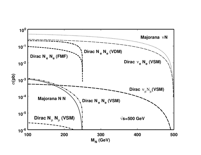
Figure 11: Single and pair production cross sections of on-shell heavy Dirac and Majorana neutrinos at $\sqrt{s}=500$ GeV for $e^{+}e^{-}$ colliders [72].

6 Extra dimensions

The possibility has recently been proposed of utilizing the geometry of extra spatial dimensions to address the hierarchy problem, i.e., the disparity between the electroweak and Planck scales [73, 74]. This idea exploits the fact that gravity has yet to be probed at energy scales much above $10^{-3}$ eV in laboratory experiments, implying that the Planck scale (of order $10^{19}$ GeV), where gravity becomes strong, may not be fundamental but simply an artifact of the properties of the higher-dimensional space. In one such scenario [73], the apparent hierarchy is generated by a large volume for the extra dimensions, while in a second case [74], the observed hierarchy is created by an exponential function of the compactification radius of the extra dimension. An exciting feature of these theories is that they afford concrete and distinctive experimental tests both in high energy physics and in astrophysics. Furthermore, if they truly describe the source of the observed hierarchy, then their signatures should appear in high-energy experiments at the TeV scale.

Another possibility is the existence of TeV^-1-sized extra dimensions accessible to Standard Model fields. Although these theories do not explicitly address the hierarchy between the Electroweak and Planck scales, they are not ruled out experimentally and may arise naturally from string theory [75]. Furthermore, they serve as a mechanism for suppressing proton decay and generating the hierarchical pattern of fermion masses [76]. Models with TeV-scale extra dimensions provide a context for new approaches to the problem of explaining electroweak symmetry breaking [77, 78] and the existence of three generations of quarks and leptons [79]. These theories also give rise to interesting phenomenology at the TeV scale.

We first describe some common features of these theories. In all the above scenarios, our universe lies on a 3+1-dimensional brane (sometimes called a wall) that is embedded in the higher $4+\delta$-dimensional space, known as the bulk. The field content that is allowed to propagate in the bulk varies between the different models. Upon compactification of the additional dimensions, all bulk fields expand into a Kaluza-Klein (KK) tower of states on the $3+1$-dimensional brane, where the masses of the KK states are related to the $\delta$-dimensional kinetic motion of the bulk field. It is the direct observation or indirect effects of the KK states that signal the existence of extra dimensions at colliders.

1 Large extra dimensions

In this scenario [73], gravitational fields propagate in the $\delta$ new large spatial dimensions, as well as in the usual $3+1$ dimensions. It is postulated that their interactions become strong at the TeV scale. The volume of the compactified dimensions, $V_{\delta}$, relates the scale where gravity becomes strong in the $4+\delta$-dimensional spaces to the apparent Planck scale via Gauss’ Law

$$M^{2}_{Pl}=V_{\delta}M_{*}^{2+\delta}\,,$$ (5)

where $M_{*}$ denotes the fundamental Planck scale in the higher-dimensional space. Setting $M_{*}$ to be of order 1 $\sim$ TeV thus determines the compactification radius $r_{c}$ ($V_{\delta}\sim r_{c}^{\delta}$) of the extra dimensions, which ranges from a sub-millimeter to a few fermi for $\delta=$ 2–6, assuming that all radii are of equal size. The compactification scale ($M_{c}=1/r_{c}$) associated with these parameters then ranges from $10^{-4}$ eV to a few MeV. The case of $\delta=1$ (which yields $r_{c}\approx 10^{11}$ m) is immediately excluded by astronomical data. Cavendish-type experiments, which search for departures from the inverse-square law gravitational force, exclude [80] $r_{c}>$ 190 $\mu$m for $\delta=2$, which translates to the bound $M_{*}>1.6$ TeV using the convention in [81]. In addition, astrophysical and cosmological considerations [82], such as the rate of supernova cooling and the diffuse $\gamma$ ray spectrum, disfavor a value of $M_{*}$ near the TeV scale for $\delta=2$. Precision electroweak data [83] do not allow the Standard Model fields to propagate in extra dimensions with $M_{c}<$ a few TeV, and hence they are constrained to the $3+1$-dimensional brane in this model.

The Feynman rules for this scenario [81, 84] are obtained by considering a linearized theory of gravity in the bulk. The bulk field strength tensor can be decomposed into spin-0, 1, and 2 states, each of which expands into KK towers upon compactification. These KK states are equally spaced and have masses of $n/r_{c}$ where $n$ labels the KK excitation level. Taking $M_{*}=1$ TeV, we see that the KK state mass splittings are equal to $5\times 10^{-4}$ eV, 20 keV, and 7 MeV for $\delta=2\,,4$, and 6, respectively. The interactions of the KK gravitons with the Standard Model fields on the wall are governed by the conserved stress-energy tensor of the wall fields. The spin-1 KK states do not interact with the wall fields because of the form of the wall stress-energy tensor. The non-decoupling scalar KK states couple to the trace of the stress-energy tensor, and are phenomenologically irrelevant for most collider processes. Each state in the spin-2 KK tower, $G_{n}$, couples identically to the Standard Model wall fields via their stress-energy tensor with the strength proportional to the inverse 4-dimensional Planck scale, $M_{Pl}^{-1}$. It is important to note that this description is an effective 4-dimensional theory, valid only for energies below $M_{*}$. The full theory above $M_{*}$ is unknown.

Two classes of collider signatures arise in this model. The first is emission of the graviton KK tower states in scattering processes [81, 85]. The relevant process at a linear collider is $e^{+}e^{-}\to\gamma/Z+G_{n}$, where the graviton appears as missing energy in the detector, behaving as if it were a massive, non-interacting, stable particle. The cross section is computed for the production of a single massive graviton excitation and then summed over the full tower of KK states. Since the mass splittings of the KK excitations are quite small compared to the collider center-of-mass energy, this sum can be replaced by an integral weighted by the density of KK states which is cut off by the specific process kinematics. The cross section for this process scales as simple powers of $\sqrt{s}/M_{*}$. It is important to note that because of the integral over the effective density of states, the emitted graviton appears to have a continuous mass distribution. This corresponds to the probability of emitting gravitons with different extra-dimensional momenta. The observables for graviton production, such as the $\gamma/Z$ angular and energy distributions, are thus distinct from those of other new physics processes, such as supersymmetric particle production, since the latter corresponds to a fixed invisible particle mass. The Standard Model background transition $e^{+}e^{-}\to\nu\overline{\nu}\gamma$ also has different characteristics, since it is a three-body process.

The cross section for $e^{+}e^{-}\to\gamma G_{n}$ as a function of the fundamental Planck scale is presented in Fig. 13 for $\sqrt{s}=1$ TeV. The level of Standard Model background is also shown, with and without electron beam polarization set at $90\%$. We note that the signal (background) increases (decreases) with increasing $\sqrt{s}$. Details of the various distributions associated with this process can be found in Cheung and Keung [85]. The discovery reach from this process has been computed in [86], with $\sqrt{s}=800$ GeV, 1000 fb^-1 of integrated luminosity, including various beam polarizations and kinematic acceptance cuts, ISR, and beamstrahlung. The results are displayed in Table 5. In this table, we have also included the $95\%$ CL bounds obtained [87] at LEP for $\sqrt{s}>200$ GeV.

The associated emission process at hadron colliders, $q\overline{q}\to g+G_{n}$, results in a mono-jet signal. In this case, the effective low-energy theory breaks down for some regions of the parameter space, as the parton-level center-of-mass energy can exceed the value of $M_{*}$. The experiment is then sensitive to the new physics appearing above $M_{*}$. An ATLAS simulation [88] of the missing transverse energy in signal and background events at the LHC with 100 fb^-1 results in the discovery range for the effective theory displayed in Table 5. The lower end of the range corresponds to values at which the ultraviolet physics sets in and the effective theory fails, while the upper end represents the boundary where the signal is no longer observable above background.

$e^{+}e^{-}\to\gamma+G_{n}$		2	4	6
LC	$P_{-,+}=0$	5.9	3.5	2.5
LC	$P_{-}=0.8$	8.3	4.4	2.9
LC	$P_{-}=0.8$, $P_{+}=0.6$	10.4	5.1	3.3
LEP II		1.45	0.87	0.61
$pp\to g+G_{n}$		2	3	4
LHC		$4.0-8.9$	$4.5-6.8$	$5.0-5.8$

Table 5: $95\%$ CL sensitivity to the fundamental Planck scale $M_{*}$ in TeV for different values of $\delta$, from the emission process for various polarization configurations and different colliders as discussed in the text. $\sqrt{s}=800$ GeV and 1 ab^-1 has been assumed for the LC and 100 fb^-1 for the LHC.

If an emission signal is observed, one would like to determine the values of the fundamental parameters, $M_{*}$ and $\delta$. In this case, measurement of the cross section at a linear collider at two different values of $\sqrt{s}$ can be used to determine $\delta$ [86] and test the consistency of the data with the hypothesis of large extra dimensions. This is displayed for a LC in Fig. 13.

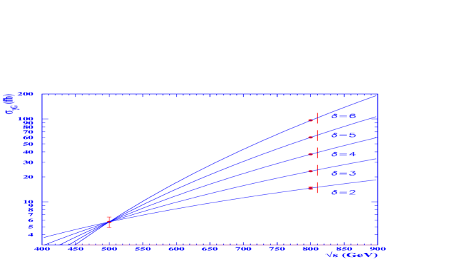
Figure 12: The cross section for $e^{+}e^{-}\to\gamma G_{n}$ for $\sqrt{s}=1$ TeV as a function of the fundamental Planck scale for various values of $\delta$ as indicated. The cross sections for the Standard Model background, with and without $90\%$ beam polarization, correspond to the horizontal lines as labeled. The signal and background are computed with the requirement $E_{\gamma}<450$ GeV in order to eliminate the $\gamma Z\to\nu\overline{\nu}\gamma$ contribution to the background. From [81].

Figure 13: The determination of $\delta$ from cross section measurements of $e^{+}e^{-}\to\gamma G_{n}$ at $\sqrt{s}=500$ and 800 GeV with 500 fb^-1 and 1 ab^-1, respectively, taking $P_{-}=80\%$ and $P_{+}=60\%$. The 500 GeV cross section has been normalized for the case $M_{*}=5$ TeV and $\delta=2$. From [82].

The second class of collider signals for large extra dimensions is that of graviton exchange [81, 84, 89] in $2\to 2$ scattering. This leads to deviations in cross sections and asymmetries in Standard Model processes such as $e^{+}e^{-}\to f\overline{f}$, and may also give rise to new production processes that are not otherwise present at tree-level, such as $e^{+}e^{-}\to hh,$ or $\tilde{g}\tilde{g}$. The exchange amplitude is proportional to the sum over the propagators for the graviton KK tower states which, as before, may be converted to an integral over the density of states. However, in this case the integral is divergent for $\delta>1$ and thus introduces a sensitivity to the unknown ultraviolet physics. Several approaches have been proposed to regulate this integral: (i) a naive cut-off scheme [81, 84, 89], (ii) an exponential damping due to the brane tension [90], (iii) restrictions from unitarity [91], or (iv) the inclusion of full weakly coupled TeV-scale string theory in the scattering process [92]. Here, we adopt the most model-independent approach, that of a naive cut-off, and set the cut-off equal to $M_{*}/\lambda^{1/4}$, where $\lambda$ accounts for the effects of the unknown ultraviolet physics. Assuming that the integral is dominated by the lowest-dimensional local operator, which is dimension-8, this results in a contact-type interaction limit for graviton exchange, which can be described via

$$i{4\lambda\over M_{*}^{4}}T^{\mu\nu}T_{\mu\nu}\,,$$ (6)

where $T^{\mu\nu}$ is the stress-energy tensor. This is described in the matrix element for $s$-channel $2\to 2$ scattering by the replacement

$${i^{2}\pi\over{M}_{Pl}^{2}}\,\sum^{\infty}_{n=1}{1\over s-m_{n}^{2}}\to{\lambda\over M_{*}^{4}}$$ (7)

with corresponding substitutions for $t$- and $u$-channel scattering. Here $m_{n}$ represents the mass of $G_{n}$, the $n^{th}$ graviton KK excitation. This substitution is universal for any $2\to 2$ process. The resulting angular distributions for fermion pair production are quartic in $\cos\theta$ and thus provide a signal for spin-2 exchange. An illustration of this is given in Fig. 15 from [89], which displays the unpolarized angular distribution as well as the angular dependence of the left-right asymmetry in $e^{+}e^{-}\to b\overline{b}$, taking $M_{*}=3\sqrt{s}=1.5$ TeV and $\lambda=\pm 1$. The two sets of data points correspond to the two choices of sign for $\lambda$, and the error bars represent the statistics in each bin for an integrated luminosity of 75 fb^-1. Here, a $60\%$ $b$-tagging efficiency, $90\%$ electron beam polarization, $10^{\circ}$ angular cut, and ISR have been included. The resulting $95\%$ CL search reach with 500 fb^-1 of integrated luminosity is given in Table 6 from summing over the unpolarized and $A_{LR}$ angular distributions for fermion ($e\,,\mu\,,\tau\,,c\,,b$ , and $t$) final states. For comparison, we also present the current bounds [87] from LEP II, HERA, and the DØ  Collaboration at the Tevatron, as well as estimates for the LHC with 100 fb^-1 [89, 93] and $\gamma\gamma$ colliders [94]. Note that the $\gamma\gamma\to WW$ process has the highest sensitivity to graviton exchange. This is due to the large $W$ pair cross section and the multitude of observables that can be formed utilizing polarized beams and $W$ decays.

The ability of the LC to determine that a spin-2 exchange has taken place in $e^{+}e^{-}\to f\overline{f}$ is demonstrated in Fig. 15 from [89]. Here, the confidence level of a fit of spin-2 exchange data to a spin-1 exchange hypothesis is displayed; the quality of such a fit is quite poor almost up to the $M_{*}$ discovery limit, indicating that the spin-2 nature is discernable.

Figure 14: Bin-integrated angular distribution and $z$-dependent ($z=\cos\theta$) left-right asymmetry for $e^{+}e^{-}\to b\overline{b}$ at $\sqrt{s}=500$ GeV. The solid histogram represents the Standard Model while the ‘data’ points are for $M_{*}=1.5$ with $\lambda=\pm 1$. The error bars indicate the statistics in each bin.

Figure 15: The percentage confidence level as a function of $M_{*}$ for a fit of spin-2 data under a spin-1 hypothesis. The dashed and solid curves correspond to the choice $\lambda=\pm 1$.

		$\sqrt{s}$ (TeV)	$M_{*}$ (TeV)
LEPII	$e^{+}e^{-}\to\ell^{+}\ell^{-},\gamma\gamma,ZZ$	0.2	1.03-1.17
LC	$e^{+}e^{-}\to f\overline{f}$	0.5	4.1
LC	$e^{+}e^{-}\to f\overline{f}$	1.0	7.2
LC	$\gamma\gamma\to WW$	1.0	13.0
LC	$\gamma\gamma\to\gamma\gamma$	1.0	3.5
LC	$e\gamma\to e\gamma$	1.0	8
HERA	$ep\to e+$ jet	0.314	0.81-0.93
Tevatron Run I	$p\overline{p}\to\ell^{+}\ell^{-},\gamma\gamma$	1.8	1.01-1.08
LHC	$pp\to\ell^{+}\ell^{-}$	14.0	7.5
LHC	$pp\to\gamma\gamma$	14.0	7.1

Table 6: $95\%$ CL search reach for $M_{*}$ from graviton exchange in various processes as indicated and discussed in the text. In the bounds from present data, a range is indicated to account for $\lambda=\pm 1$.

The scenario with large extra dimensions resolves the hierarchy problem without invoking supersymmetry. However, if this mechanism is embedded in a string theory, then supersymmetry may also be present at the weak scale. A supersymmetric bulk then results in a KK tower of gravitinos, in addition to the KK gravitons. In supersymmetric models that expect a light gravitino, such as gauge-mediated supersymmetry breaking, the gravitino KK tower can yield interesting phenomenological effects. An example of this is in the process $e^{+}e^{-}\to\tilde{e}^{+}\tilde{e}^{-}$, which would now also receive contributions from $t$-channel KK gravitino exchange and $s$-channel KK graviton exchange. This has been studied in [95], which considered an $N=2$ supersymmetry in the bulk, and after compactifying the gravitino sector, derived the KK gravitino couplings to $N=1$ supersymmetric matter on the brane. The resulting dramatic effect on selectron pair production is highlighted by the ability to select various production channels via the use of electron beam polarization. This is displayed in Fig. 16, which shows the binned angular distribution for $e^{-}_{L,R}e^{+}\to\tilde{e}_{L}^{\mp}e_{R}^{\pm}$ for various values of $M_{*}$; this choice of polarization isolates the $t$-channel neutralino and KK gravitino contributions. The search reach for this process at $\sqrt{s}=500$ GeV with $80\%$ beam polarization and 500 fb^-1 of integrated luminosity is $M_{*}\sim 12$ TeV for the case $\delta=6$.

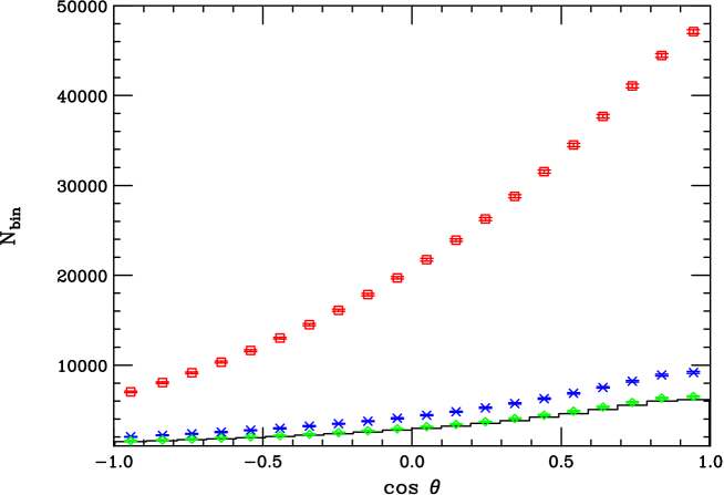
Figure 16: The number of events per bin in $e^{-}_{L,R}e^{+}\to\tilde{e}_{L}^{\mp}\tilde{e}_{R}^{\pm}$ for $\sqrt{s}=500$ GeV with 500 fb^-1 of integrated luminosity and $P_{-}=80\%$. The curves correspond to $M_{*}=1.5\,,3\,,6$ TeV from top to bottom with the solid histogram representing the minimal supersymmetric case. The error bars correspond to the statistics in each bin. Here the values $m_{\tilde{e}_{L}}=220$ GeV and $m_{\tilde{e}_{R}}=117$ GeV are assumed.

2 Localized gravity

We now turn to the scenario where the hierarchy is generated by an exponential function of the compactification radius. In its simplest form, gravity propagates in the bulk, while the Standard Model fields are constrained to a 3-brane. This model contains a non-factorizable geometry embedded in a slice of 5-dimensional Anti-de Sitter space (AdS₅), which is a space of negative curvature. Two 3-branes reside rigidly at fixed points at the boundaries of the AdS₅ slice, located at $|\phi|=0,\pi$ where $\phi$ parameterizes the fifth dimension. The 5-dimensional Einstein equations permit a solution that preserves 4-d Poincaré invariance with the metric

$$ds^{2}=e^{-2kr_{c}|\phi|}\eta_{\mu\nu}dx^{\mu}dx^{\nu}-r_{c}^{2}d\phi^{2}\,,$$ (8)

where $\pi r_{c}$ is the length of the fifth dimenion. The exponential function, or warp factor, multiplying the usual 4-d Minkowski term curves space away from the branes. The constant $k$ is the AdS₅ curvature scale, which is of order the Planck scale and is determined by the bulk cosmological constant. The scale of physical phenomena as realized by the 4-d flat metric transverse to the fifth dimension is specified by the exponential warp factor. If the gravitational wavefunction is localized on the brane at $\phi=0$ (called the ‘Planck brane’), then TeV scales can naturally be attained [74] on the 3-brane at $\phi=\pi$ (the ‘TeV brane’, where the Standard Model fields reside) if $kr_{c}\simeq$ 11–12. The scale $\Lambda_{\pi}\equiv\overline{M}_{Pl}e^{-kr_{c}\pi}\sim 1$ TeV, where $\overline{M}_{Pl}=M_{Pl}/\sqrt{8}\pi$ is the reduced Planck scale, then describes the scale of all physical processes on the TeV-brane. We note that it has been demonstrated [96] that this value of $kr_{c}$ can be stabilized without fine tuning of parameters.

Two parameters govern the 4-d phenomenology of this model, $\Lambda_{\pi}$ and the ratio $k/\overline{M}_{Pl}$. Constraints on the curvature of the AdS₅ space suggest that $k/\overline{M}_{Pl}\mathrel{\raise 1.29167pt\hbox{$<$\kern-7.5pt\lower 4.30554pt\hbox{$\sim$}}}0.1$. The Feynman rules are obtained by a linear expansion of the flat metric, including the warp factor. After compactification, a KK tower of gravitons appears on the TeV-brane and has masses $m_{n}=x_{n}ke^{-kr_{c}\pi}=x_{n}\Lambda_{\pi}k/\overline{M}_{Pl}$ with the $x_{n}$ being the roots of the first-order Bessel function, i.e., $J_{1}(x_{n})=0$. Note that the first excitation is naturally of order a few hundred GeV and that the KK states are not evenly spaced. The interactions of the graviton KK tower with the Standard Model fields on the TeV brane are [97]

$${\cal L}=-{1\over\overline{M}_{Pl}}T^{\mu\nu}(x)h^{(0)}_{\mu\nu}(x)-{1\over\Lambda_{\pi}}T^{\mu\nu}(x)\sum^{\infty}_{n=1}h^{(n)}_{\mu\nu}(x)\,,$$ (9)

where $T^{\mu\nu}$ is the stress-energy tensor. Note that the zero-mode decouples and that the couplings of the higher states have inverse-TeV strength. This results in a strikingly different phenomenology from the case of large extra dimensions. Here, the graviton KK tower states are directly produced as single resonances if kinematically allowed.

If the KK gravitons are too massive to be produced directly, their contributions to fermion pair production may still be felt via virtual exchange. In this case, the uncertainties associated with the introduction of a cut-off are avoided, since there is only one additional dimension and the KK states may be neatly summed. The sensitivity [97] to $\Lambda_{\pi}$ at a linear collider for various values of $k/\overline{M}_{Pl}$ is listed in Table 7 for 500 fb^-1 of integrated luminosity. For purposes of comparison, the corresponding reach at LEP II, Tevatron Run II, and the LHC is also displayed.

With sufficient center-of-mass energy the graviton KK states may be produced as resonances. To exhibit how this may appear at a linear collider, Fig. 17 displays the cross section for $e^{+}e^{-}\to\mu^{+}\mu^{-}$ as a function of $\sqrt{s}$, assuming $m_{1}=500$ GeV and taking $k/\overline{M}_{Pl}=$0.01–0.05. The height of the third resonance is somewhat reduced, because the higher KK excitations decay to the lighter graviton states once it is kinematically allowed [98]. In this case one can study graviton self-couplings, and higher-energy $e^{+}e^{-}$ colliders may become graviton factories!

Searches for the first graviton KK resonance in Drell-Yan and di-jet data at the Tevatron already place non-trivial restrictions [97] on the parameter space of this model, given roughly by $m_{1}\mathrel{\raise 1.29167pt\hbox{$>$\kern-7.5pt\lower 4.30554pt\hbox{$\sim$}}}$ 175, 550, 1100 GeV for $k/\overline{M}_{Pl}=0.01\,,0.1\,,1.0$. Precision electroweak data extend [99] this search reach for smaller values of $k$. These constraints, taken together with the theoretical prejudices that (i) $\Lambda_{\pi}\mathrel{\raise 1.29167pt\hbox{$<$\kern-7.5pt\lower 4.30554pt\hbox{$\sim$}}}10$ TeV, i.e., the scale of physics on the TeV brane is not far above the electroweak scale and (ii) $k/\overline{M}_{Pl}\mathrel{\raise 1.29167pt\hbox{$<$\kern-7.5pt\lower 4.30554pt\hbox{$\sim$}}}0.1$ from the above-mentioned AdS₅ curvature considerations, result in a closed allowed region in the 2-dimensional parameter space, which can be completely explored at the LHC [99, 100] via the Drell-Yan mechanism.

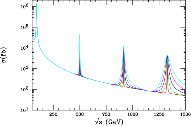
Figure 17: The cross section for $e^{+}e^{-}\to\mu^{+}\mu^{-}$ including the exchange of a KK tower of gravitons with $m_{1}=500$ GeV. The curves correspond to $k/\overline{m}_{Pl}=$ in the range 0.01–0.05.

	$k/\overline{M_{Pl}}$
	0.01	0.1	1.0
LC $\sqrt{s}=0.5$ TeV	20.0	5.0	1.5
LC $\sqrt{s}=1.0$ TeV	40.0	10.0	3.0
LEP II	4.0	1.5	0.4
Tevatron Run II	5.0	1.5	0.5
LHC	20.0	7.0	3.0

Table 7: $95\%$ CL search reach for $\Lambda_{\pi}$ in TeV in the contact interaction regime taking 500, 2.5, 2, and 100 fb^-1 of integrated luminosity at the LC, LEP II, Tevatron, and LHC, respectively. From [97].

Lastly, we note that if the Standard Model fields are also allowed to propagate in the bulk [99, 101], the phenomenology can be markedly different, and is highly dependent on the value of the 5-dimensional fermion mass. For various phenomenological reasons, it is least problematic to keep the Higgs field on the TeV brane [101]. As a first step, one can study the effect of placing the Standard Model gauge fields in the bulk and keeping the fermions on the TeV-brane. In this case, the fermions on the wall couple to the KK gauge fields a factor of $\sqrt{2kr_{c}\pi}\sim 9$ times more strongly than they couple to the ($\gamma,g,W^{\pm},Z$). In this case, precision electroweak data place strong constraints, requiring that the lightest KK gauge boson have a mass greater than about 25 TeV. This value pushes the scale on the TeV-brane above 100 TeV, making this scenario disfavored in the context of the hierarchy problem.

This bound can be relaxed if the fermions also reside in the bulk [101]. By introducing bulk fermion 5-d masses $m_{5}$, the couplings of the fermion zero modes (i.e., the Standard Model fermions) to various KK fields become a function of the bulk mass parameter $\nu\equiv m_{5}/k$. The parameter $\nu$ controls the shape of the fermion zero-mode wavefunction, with negative (positive) values of $\nu$ serving to localize the wavefunction near the Planck brane (TeV brane). Constraints from avoiding flavor-changing neutral currents, Yukawa coupling blow-up, and the generation of a new hierarchy result in a rather narrow allowed range of $\nu$. For some values of $\nu$ in this range, the fermionic couplings of the KK graviton states essentially vanish, and hence the graviton production mechanisms discussed above are no longer viable. In this case, the gravitons retain a small coupling to the Standard Model gauge bosons, and the most promising production mechanism [99] is at a photon collider via $\gamma\gamma\to G_{n}\to hh$, with $h$ being the Higgs boson.

3 TeV-scale extra dimensions

TeV^-1-sized extra dimensions can naturally arise in some string theory models [75], and in this case, the Standard Model fields may feel their effects. The physics of models with KK excitations of the Standard Model gauge bosons arising from TeV-scale extra dimensions has been discussed for some time [102]. The various models in this class of theories differ in detail in two regards: ($i$) the placement of the Higgs field(s) in the bulk or on the wall(s), and ($ii$) the treatment of the fermion fields.

If Higgs fields propagate in the bulk, the expectation value of the zero-mode field generates electroweak symmetry breaking. In this case, there is no mixing among the various gauge boson KK modes. Thus the KK mass matrix is diagonal, with the masses of the excitations given by $[M_{0}^{2}+\vec{n}\cdot\vec{n}M_{c}^{2}]^{1/2}$, where $M_{0}$ is the zero-mode mass, $M_{c}$ is the compactification mass scale and $\vec{n}$ is a set of integers labeling the excitation state. However, if the Higgs is a wall field, its expectation value induces off-diagonal elements in the mass matrix and thus a mixing among the gauge KK states. In this case the mass matrix needs to be diagonalized to determine the masses and couplings of the gauge KK states. It is also possible to imagine a more generalized mixed scenario with two Higgs fields, one residing in the bulk and one on the wall, that share the SM symmetry breaking. Clearly, the detailed phenomenology of these possibilities will be quite different. For example, a small mixing of the gauge KK states may show up in precision measurements when $W$ and $Z$ properties are compared with Standard Model expectations.

An even more diverse situation arises when one considers the placement of the Standard Model fermions within the extra dimensions. There are essentially three possibilities:

$(a)$ The fermions are constrained to 3-branes located at fixed points. This is the most common situation discussed in the literature [83] and in this case the fermions are not directly affected by the extra dimensions. For models in this class, global fits to precision electroweak data place strong lower bounds on the value of $M_{c}$, which corresponds to the mass of the first gauge KK excitation. Following the analysis of Rizzo and Wells [83] and employing the most recent data [103], one finds that $M_{c}>4.4$ TeV when the Higgs field is on the wall; the bound is 4.6 TeV when the Higgs field is in the bulk. Such a large mass for gauge KK states is beyond the direct reach of a LC, but the KK states can be directly produced as resonances at the LHC in the Drell-Yan channel provided that $M_{c}\mathrel{\raise 1.29167pt\hbox{$<$\kern-7.5pt\lower 4.30554pt\hbox{$\sim$}}}6$ TeV. This reach at the LHC may be extended by a TeV or so [104] by examination of the Drell-Yan line shape at high lepton-pair invariant mass. However, the LC can indirectly observe the existence of heavy gauge KK states via their $s$-channel exchanges in the contact interaction limit. Combining the results from various fermion final states in $e^{+}e^{-}\to f\overline{f}$ gives the $95\%$ CL search reach displayed in Table 8.

	$M_{c}$ Reach (TeV)
Tevatron Run II 2 fb-1	1.1
LHC 100 fb-1	6.3 ($\sim$ 7.5)
LEP II	3.1
LC $\sqrt{s}=0.5$ TeV 500 fb-1	13.0
LC $\sqrt{s}=1.0$ TeV 500 fb-1	23.0
LC $\sqrt{s}=1.5$ TeV 500 fb-1	31.0

Table 8: $95\%$ CL search reach for the mass of the first KK gauge boson excitation. From Rizzo and Wells [83]. The LHC reach is via direct observation of a resonance, while the LC sensitivities are from indirect effects as in the case of a search for a new neutral gauge boson. The number in parentheses for the LHC is an estimate of the extension of the complete search reach including indirect effects from contact interactions.

If a $\gamma^{(1)}/Z^{(1)}$ KK resonance is observed at the LHC, a $\sqrt{s}=500$ GeV linear collider can distinguish this state from a new neutral gauge boson arising from an extended gauge sector by using the Bhabha scattering channel. If one attempts to fit the induced deviations in the Bhabha cross section and polarized asymmetry by varying the vector and axial-vector couplings of a hypothetical non-KK $Z^{\prime}$, one finds [105] that the CL of the fit is quite poor ($\mathrel{\raise 1.29167pt\hbox{$<$\kern-7.5pt\lower 4.30554pt\hbox{$\sim$}}}10^{-3}$). This demonstrates that the assumption that the KK state is a $Z^{\prime}$ is incorrect. A separate fit assuming that the resonance is a KK state yields a good fit. At the LHC, it is currently unclear whether the $\gamma^{(1)}/Z^{(1)}$ KK resonance can be distinguished from a $Z^{\prime}$ in a model-independent manner.

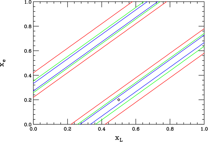
Figure 18: The ability of a LC to determine the separation in the extra dimension of right- and left-handed electrons from Bhabha scattering. The red, green, and blue (outer, middle, and inner) set of curves correspond to $\sqrt{s}=$ 500, 1000, 1500 GeV, respectively, with 500 fb^-1 assumed for each energy. This case assumes $M_{c}=4$ TeV and that the location of the right- (left-)-handed electron, $x_{e(L)}$, is given by a Gaussian centered at $0.2\ (0.5)\cdot 2\pi r_{c}$.

($b$) The Standard Model fermions are localized at specific points, $x_{i}$, in the extra TeV dimension, which are not necessarily at the orbifold fixed points. Here, the zero- and excited-mode fermions obtain narrow Gaussian-like wave functions in the extra dimensions with a width $\sigma$ much smaller than the compactification scale, i.e., $(\sigma/\pi r_{c})^{2}\ll 1$. The placement of SM fermions at different locations and the narrowness of their wavefunctions can then suppress [76] the rates for a number of dangerous processes such as proton decay. For the lighter gauge KK modes (small values of $n$), the width of the fermion wavefunction centered at a given point cannot be resolved, so that the wavefunction appears similar to a delta function. Thus the coupling of the fermion to these gauge KK states is determined by the value of the gauge KK wavefunction evaluated at that point. However, when $n\sigma/\pi r_{c}$ grows to order unity or larger, the KK gauge field can resolve the finite size of the fermion wavefunction and the coupling of the fermion becomes exponentially damped. This decouples the heavy gauge KK states, providing a means of rendering sums over KK towers of gauge bosons finite in the case of two or more extra dimensions [106]. An analysis of precision electroweak data in this case shows that $M_{c}$ is typically found to be $\geq 3-4$ TeV. Depending upon the properties of the compactification manifold, measurements at colliders may probe the distance in the extra dimensions between two fermions, $|x_{i}-x_{j}|$, in $2\to 2$ scattering. For example, in this case Bhabha scattering can probe the distance between the left- and right-handed electrons, as illustrated in Fig. 18. A study of the cartography of the localized fermions at linear colliders has been performed in [107]. At very large energies, the cross section for the polarized version of this process will tend rapidly to zero since the two particles completely miss each other in the extra dimension [108].

($c$) The fermions are fields in the bulk. This possibility is known as the ‘universal extra dimensions’ scenario [109]. This case is different in that walls or branes are not present and hence momentum is conserved in the additional dimensions. The consequence of this is that KK number is conserved at all interaction vertices, hence only pairs of KK gauge bosons couple to the zero-mode fermions. In this case, electroweak precision data as well as direct searches for KK states lead to a reduced lower bound of $M_{c}\simeq 0.4$ TeV. Without further ingredients, this model may have trouble satisfying cosmological constraints, since the lightest KK excitations are absolutely stable. This may be avoided if there is any small breaking of translation invariance in the extra dimensions. Alternatively, one can imagine the gauge and fermion KK fields as confined to a brane of thickness TeV^-1, i.e., a thick brane, embedded in a highe-dimensional space that includes gravity. In this case the higher-level KK modes can decay down to the zero modes via graviton emission, but at a rate determined by the ‘form factor’ of the brane [110]. In either case an interesting phenomenology results. The KK states are produced in pairs at colliders and then either decay via one of these two mechanisms or are long-lived and appear as tracks in a detector.

7 Highly non-conventional theories and possible surprises

So far in this chapter, we have delineated the potential of a linear collider to explore the new physics that is present in set classes of established models. However, as likely as not, when Nature finally reveals her mysteries they will be full of surprises that lie outside the realm of our limited imaginations.

Along these lines, we note that some of the most striking recent developments have occured in string theory. While it is currently difficult to relate these theories to experiment, some of their ingredients, when considered on their own, have interesting phenomenological consequences. Here, we consider two such examples of this top-down approach, as a demonstration of the potential of the LC to discover the unforseen.

1 String resonances

If the scenario with large extra dimensions discussed in a previous section is embedded in a string theory, then stringy effects must also appear at the TeV scale. Hence, not only the gravitons, but also the Standard Model fields must have an extended structure. The exchange of string Regge excitations of Standard Model particles in $2\to 2$ scattering may appear as contact-like interactions with a strength that overwhelms the corresponding graviton exchange. This is deduced from simple coupling-counting arguments. Yang-Mills bosons live at the end of open strings, while gravitons correspond to closed string states, which require an additional coupling constant factor at the amplitude level. Hence the exchange of KK graviton states is suppressed by a factor of $g^{2}$ compared to the exchange of string Regge excitations.

This has been examined in [111], where an illustrative string model was assumed. This model makes use of scattering amplitudes on the 3-brane of weakly coupled type IIB string theory to describe a string version of QED. Electrons and photons then correspond to massless states of open strings ending on the 3-brane and are characterized by the quantum theory of fluctuations of an open string with specified boundary conditions. Within the context of this model, Bhabha scattering and pair annihilation receive contributions from the string Regge exchanges. The differential cross section for these processes is modified by a form factor,

$${d\sigma\over d\cos\theta}=\left({d\sigma\over d\cos\theta}\right)_{SM}\left|{\Gamma(1-s/M^{2}_{str})\Gamma(1-t/M^{2}_{str})\over\Gamma(1-s/M^{2}_{str}-t/M^{2}_{str})}\right|^{2}\,,$$ (10)

which essentially mirrors the original Veneziano result [112]. Here, $M_{str}$ represents the string scale and can be related to the fundamental Planck scale in the large extra dimension scenario via $M_{*}/M_{str}=\pi^{-1/8}\alpha^{-1/4}$. Figure 19 displays the deviation from Standard Model expectations to Bhabha scattering from these string exchanges, and compares their effect to those arising from other types of contact interactions. The 95% CL exclusion limits for $\sqrt{s}=1$ TeV and 200 fb^-1 is $M_{str}>3.1$ TeV, which corresponds to $M_{*}/\lambda^{1/4}>9.3$ TeV.

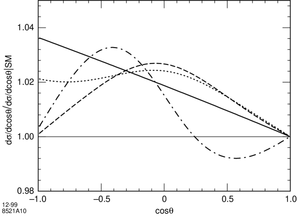
Figure 19: Comparison of deviations from the Standard Model prediction for Bhabha scattering at 1 TeV due to corrections from higher-dimension operators [111]. The curves correspond to: string model with $M_{str}=3.1$ TeV (solid), KK graviton exchange with $M_{*}/\lambda^{1/4}=6.2$ TeV (dotted), VV contact interactions with $\Lambda=88$ TeV (dashed), and AA contact interactions with $\Lambda=62$ TeV (dot-dashed).

2 Non-commutative field theories

Recent theoretical results have demonstrated that non-commutative quantum field theories (NCQFT) naturally appear within the context of string theory and M-theory [113]. In this case, the usual $\delta$-dimensional space associated with commuting space-time coordinates is generalized to one that is non-commuting. In such a space, the conventional coordinates are represented by operators that no longer commute,

$$[\hat{X}_{\mu},\hat{X}_{\nu}]=i\theta_{\mu\nu}\equiv{i\over\Lambda^{2}_{NC}}c_{\mu\nu}\,.$$ (11)

Here, the effect has been parameterized in terms of an overall scale $\Lambda_{NC}$, which characterizes the threshold where non-commutative (NC) effects become important, and a real antisymmetric matrix $c_{\mu\nu}$, whose dimensionless elements are presumably of order unity. The most likely value of $\Lambda_{NC}$ is near the string scale or the true Planck scale, which could be as low as the TeV scale. The matrix $c_{\mu\nu}$ is related to the Maxwell field-strength tensor $F_{\mu\nu}$ in a straightforward fashion, since NCQFT arises in string theory in the presence of background electromagnetic fields. The matrix $c_{\mu\nu}$ is identical in all reference frames, defining a preferred NC direction in space, and hence Lorentz invariance is violated at energies of order $\Lambda_{NC}$. The usual description of Lorentz violation needs to be modified in order to apply to NCQFT; present experiments only constrain such effects at the few-TeV level [114].

Caution must be exercised to preserve orderings of the products of fields when formulating NCQFT. This is accomplished with the introduction of the star product, $\phi(\hat{X})\phi(\hat{X})=\phi(x)*\phi(x)=\phi(x)e^{[i\theta^{\mu\nu}\partial_{\mu}\partial_{\nu}/2]}\phi(x)$, which absorbs the effect of the commutation relation via a series of Fourier transforms. The NC action for a quantum field theory is thus obtained from the ordinary one by replacing the products of fields by star products. A striking consequence of this is that the NC version of QED takes on a non-Abelian nature in that both 3-point and 4-point photon couplings are generated. In addition, all QED vertices pick up additional phase factors that are dependent upon the momenta flowing through the vertex. We note that propagators, however, are not modified since quadratic forms remain unchanged under the properties of the star product. NC effects thus produce striking signatures in QED processes at a linear collider. The modifications to pair annihilation, Bhabha and Møller scattering, as well as $\gamma\gamma\to\gamma\gamma$ have been studied in [115]. Pair annihilation and $\gamma\gamma$ scattering both receive new diagrammatic contributions due to the non-Abelian couplings, and all four processes acquire a phase dependence due to the relative interference of the vertex kinematic phases. The lowest-order correction to the Standard Model in these processes occurs at dimension 8. The most striking result is that a $\phi$ dependence is induced in $2\to 2$ scattering processes because of the existence of the NC preferred direction in space-time. This azimuthal dependence in pair annihilation is illustrated in Fig. 20 for the case where the NC direction is perpendicular to the beam axis. The results of [115] are summarized in Table 9, which displays the $95\%$ CL search reach for the NC scale in these four reactions. We see that these processes are complementary in their ability to probe different structures of non-commuting space-time.

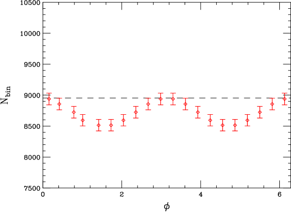
Figure 20: $\phi$ dependence of the $e^{+}e^{-}\rightarrow\gamma\gamma$ cross section, taking $\Lambda_{NC}={\sqrt{s}}=500$ GeV a luminosity of $500\,{\rm fb}^{-1}$. A cut of $|\cos\theta|<0.5$ has been employed. The dashed line corresponds to the SM expectations and the ‘data’ points represent the NCQED results.

Process	Structure Probed	Bound on $\Lambda_{NC}$
$e^{+}e^{-}\to\gamma\gamma$	Space-Time	$740-840$ GeV
Møller Scattering	Space-Space	1700 GeV
Bhabha Scattering	Space-Time	1050 GeV
$\gamma\gamma\to\gamma\gamma$	Space-Time	$700-800$ GeV
	Space-Space	500 GeV

Table 9: Summary of the $95\%$ CL search limits on the NC scale $\Lambda_{NC}$ from the various processes considered above at a 500 GeV linear collider with an integrated luminosity of 500 fb^-1.

Figure 21: Results of the fit with 95% CL contours circled around the fitted values. The box in the center corresponds to the Standard Model, the dotted ellipses represent the fit to the four $Z^{\prime}$ cases considered, and the dashed ellipse is for the case of sneutrino exchange. The fit was performed taking $\sqrt{s}=1$ TeV with 150 fb^-1.

8 Determining the origin of new physics

As demonstrated in this chapter, some reactions at linear colliders may receive contributions from many different models. An example of this is $e^{+}e^{-}\rightarrow f\overline{f}$, in which indirect effects of compositeness, extended gauge sectors, extra dimensions, string resonances, or supersymmetry may be revealed. Once a signal for new physics is found, the next step is to unravel the properties associated with the new phenomena. If the mass spectrum of the new particles in these theories is kinematically accessible, then their properties may be directly measured. However, if these states are too heavy, then we must explore their characteristics indirectly. This is feasible at a linear collider because of the precision at which measurements can be performed. Here, we give a single example to illustrate our point, namely, the ability of $e^{+}e^{-}$ colliders to provide unique information about the spin structure of new objects. The angular distributions and polarization asymmetries associated with $e^{+}e^{-}\rightarrow f\overline{f}$ are sensitive probes of the spin of new particles. An illustration of this was presented in Fig. 15, which showed the extent to which spin-2 exchange in $e^{+}e^{-}\rightarrow f\overline{f}$ is distinguishable from other new physics sources. This figure showed that deviations induced by spin-2 graviton exchanges can be distinguished from those due to lower spins, such as new vector bosons $Z^{\prime}$ or a scalar neutrino in R-parity-violating models, up to the discovery limit. In addition, discrimination between spin-1 and spin-0 particles at a LC was demonstrated [116] by studying the angular distributions induced by the exchange of a $Z^{\prime}$ and of a scalar neutrino, $\tilde{\nu}$ in $e^{+}e^{-}\rightarrow f\overline{f}$. A two-parameter fit of a trial distribution of the form $\sim A(1+z)^{2}+B(1-z)^{2}$ was performed to the observables, with $A,B$ being parameters determined by the fit. In the case of the Standard Model and $Z^{\prime}$, the fitted parameters $A,B$ are constant, while, in the case of $\tilde{\nu}$, the parameter $B$ depends on $z$. The results of the fit are displayed in Fig. 21. The Standard Model values of $A$ and $B$ are shown in the center of the figure and are assumed to be known precisely. The $Z^{\prime}$ mass was set to 3 TeV and four different $Z^{\prime}$ coupling values were considered. The $\tilde{\nu}$ was allowed to mediate the reaction in both $s$- and $t$-channels. All five regions are statistically well separated from each other, and clearly distant from the Standard Model solution.

9 Conclusions

In this chapter, we have discussed several classes of motivated models that contain new phenomena, and we have delineated the ability of a linear collider to explore them. We have seen that the LHC and the linear collider have a comparable and complementary discovery potential. In many cases, a signal for new physics will first be observed at the LHC, and the linear collider will precisely determine its properties. While a 500 GeV linear collider has a large discovery reach and potential to elucidate the underlying physics, every physics scenario we have also explored benefits from an upgrade to higher energy.

However, our limited imagination does not span the full range of alternatives allowed by present data. We thus must be prepared to discover the unexpected, which is best accomplished by exploration of the energy frontier by both $e^{+}e^{-}$ and hadron colliders.

Chapter 6 Top Quark Physics

1 Introduction

The linear collider, operating near the $t\overline{t}$ production threshold and at higher energies, can carry out a comprehensive program of top quark physics. Measurements at the threshold include the determination of the top quark mass, $m_{t}$, and width, $\Gamma_{t}$, as well as the top quark Yukawa coupling, $g_{tth}$. The quantities $m_{t}$ and $g_{tth}$ can also be measured at higher energies, together with the couplings of the top quark to the electroweak gauge bosons. In this chapter we present a brief summary of our current understanding of top quark physics at a linear collider.

The top is unique among the quarks in that it decays before nonperturbative strong interaction effects can influence it. Its large mass gives it stronger coupling to many proposed new physics effects that try to explain electroweak symmetry breaking and/or the origin of particle masses. Thus, precise measurement of the parameters of the top quark would provide important insights into physics beyond the Standard Model.

2 Physics in the threshold region

1 Introduction

One of the primary goals of a high-energy $e^{+}e^{-}$ linear collider is the study of sharp features in the cross section for $e^{+}e^{-}$ annihilation to hadrons. The $t{\overline{t}}$ threshold is an excellent example of such a structure. The cross section for $e^{+}e^{-}\to t\overline{t}$ is expected to rise by an order of magnitude with only a 5 GeV change in center-of-mass energy around 350 GeV. Careful study of this $t{\overline{t}}$ threshold structure can precisely measure many parameters of the top quark, including its mass and width, and the top quark Yukawa coupling. In this section we briefly summarize the current status of $t\overline{t}$ threshold studies. More comprehensive discussions can be found in [2, 3, 4].

2 QCD dynamics and cross section

It is well known that, because of the large top quark width ($\Gamma_{t}\approx 1.4{\rm\,GeV}\gg\Lambda_{QCD}$), a top-antitop pair cannot form narrow toponium resonances. Instead, the cross section is expected to have a smooth line-shape showing only a moderate $1S$ peak. The dynamics of the top quark in the threshold region is described by perturbative QCD. The top quark width serves as an infrared cutoff. As a result, nonperturbative QCD effects (as measured, for example, by the influence of the gluon condensate) are small [5], allowing us, in principle at least, to calculate the cross section from QCD with high accuracy.

The convergence of QCD perturbation theory in the threshold region depends on the quark mass definition used. The simplest definition of $m_{t}$ is the position of the pole in the top quark propagator. This ‘pole mass’ is similar to the kinematic mass observed in top quark pair production above threshold, and similar to the mass definition used by the CDF and DØ experiments in the original papers on the top quark discovery [6, 7]. Unfortunately, with this choice of the mass definition, the NNLO corrections are uncomfortably large [2] and shift the $1S$ peak by about $0.5{\rm\,GeV}$, spoiling the possibility to extract the top quark mass with high accuracy. The threshold cross sections computed at successive order in QCD are shown in the left-hand graph in Fig. 1. The instability of this perturbation series is caused by the fact that the pole mass has a renormalon ambiguity, that is, it obtains an additive correction from nonperturbative QCD effects.

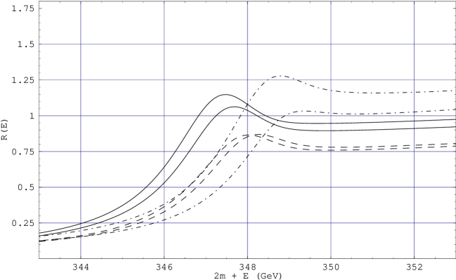
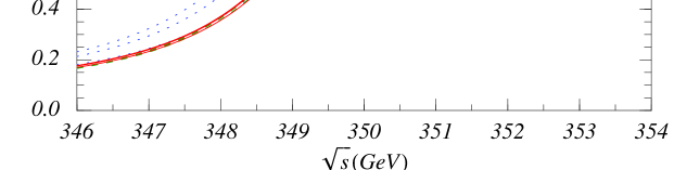
Figure 1: The normalized cross section $R_{t}=\sigma(e^{+}e^{-}\to t\overline{t})/\sigma(e^{+}e^{-}\to\mu^{+}\mu^{-})$ as a function of $\sqrt{s}$, computed in QCD perturbation theory at various levels. These are theoretical curves that do not include initial state radiation, beamstrahlung, or beam energy spread. (Left:) The normalized cross section computed with the pole mass $m^{\rm pole}_{t}=175$ GeV, at LO (dashed-dotted lines), NLO (dashed lines), and NNLO (solid lines). Each pair of the curves corresponds to the two different soft normalization scales $\mu=30$ GeV (upper curve) and $\mu=60$ GeV (lower curve). (Right:) The normalized cross section computed with the $1S$ mass $m_{t}^{1S}=175$ GeV, at LL order (dotted), NLL order (dashed) and NNLL order in QCD (solid). The calculation includes the summation of logarithms of the top quark velocity, and at each order curves are shown for $\nu=0.15,0.2,0.4$, where $\nu$ is the so-called subtraction velocity.

To remove this difficulty, one can use a different mass definition that refers only to short-distance QCD physics. For example, a possible definition of the mass, called the $1S$ mass, is one-half of the mass of the lowest toponium bound state computed in the hypothetical limit of zero top quark width [8]. Three other mass definitions have been considered in the literature. The $\overline{\rm PS}$ mass [9] is defined via the top quark self-energy. The $LS$ (‘low scale’) mass is given in terms of perturbative evaluations of matrix elements of operators in the heavy quark effective theory that describe the difference between the pole mass and a fictitious $T$ meson mass [10]. Finally, the PS (‘potential-subtracted’) mass is defined by

$$m_{t}^{PS}(\mu)=m_{t}^{\rm pole}+\frac{1}{2}\int\limits_{|k|<\mu}\frac{d^{3}k}{(2\pi)^{3}}V_{C}(k)=m_{t}^{\rm pole}-\frac{4}{3}\frac{\alpha_{s}}{\pi}\mu+...$$ (1)

where $\mu$ is the soft renormalization scale. All of these mass definitions, collectively called ‘threshold masses’ have the property that they are free of the ${\cal O}(\Lambda_{QCD})$ renormalon ambiguity [11, 12]. These masses also have the property that they are connected to the $\overline{MS}$ top quark mass by a convergent QCD perturbation series.

The position of the $1S$ peak becomes much more stable at higher orders of QCD if threshold masses are used. The shifts from order to order are less than 100 MeV. However, a large theoretical normalization uncertainty of about 10% remains. The normalization uncertainty can be reduced to a few percent by resumming terms logarithmic in the top velocity. The convergence for the $1S$ mass definition is shown in the right-hand graph of Fig. 1 [13]. Simultaneous accurate measurements of the top mass and other quantities thus appear feasible, as discussed further below.

3 Top width

The scan of the $t\overline{t}$ threshold will allow a direct measurement of the top quark width, $\Gamma_{t}$. The cross section at the $1S$ quarkonium bound state energy is proportional to $1/\Gamma_{t}$. Realistic studies, which include initial state radiation and other effects, show that $\Gamma_{t}$ can be measured with an experimental precision of a few percent [3], now that higher-order QCD corrections appear to be under control [13].

$\Gamma_{t}$ can also be measured using the forward-backward asymmetry [14]. The $t\overline{t}$ vector coupling to $\gamma$ and $Z$ produces mainly S-wave states, while the axial-vector coupling from the $Zt\overline{t}$ vertex produces $t\overline{t}$ in a P state. The top quark width causes the S and P states to overlap and allows these states to interfere in the final angular distribution. This produces a forward-backward asymmetry. Since the top quark width controls the amount of S-P overlap, the asymmetry is sensitive to $\Gamma_{t}$. Realistic studies are needed to better quantify the experimental sensitivity.

4 Top quark Yukawa coupling

In addition to the QCD potential, the $t\overline{t}$ pair interacts via a Yukawa potential associated with Higgs boson exchange

$$V_{tth}=-\frac{g_{tth}^{2}}{4\pi}~{}\frac{e^{-m_{h}r}}{r},$$ (2)

where $m_{h}$ is the Higgs boson mass and $g_{tth}$ is the Yukawa coupling. Therefore, top threshold measurements can also be used to determine $g_{tth}$ if the Higgs boson is light. A SM Higgs boson with a mass of 115 GeV enhances the normalization of the cross section by 5–8% at energies near the threshold. The theoretical uncertainty of the cross section in this region is 2–3% when the summation of logarithms of the top quark velocity is taken into account [13]. A precision measurement of the $t{\overline{t}}$ threshold cross section thus will be sensitive to the top Yukawa coupling. If we fix all other parameters and assume $m_{h}=115\,{\rm GeV}$, then varying the SM Yukawa coupling by $\pm 14\%$ gives a $\pm 2\%$ variation in the normalization of the cross section near the $1S$ peak [15]. For larger values of $m_{h}$, the sensitivity to $g_{tth}$ is expected to decrease. Again, realistic experimental studies that make use of recent theoretical advances in understanding the threshold cross section are needed.

5 Experimental issues

The experimental situation of the $t{\overline{t}}$ threshold is fairly well understood, and there has not been much progress since the experimental methods were reviewed at the 1999 Sitges meeting [16]. It is expected that the top mass can be measured with a statistical uncertainty of 40 MeV in a modest scan of 10 fb^-1, a small fraction of a year at typical design luminosities. A longer scan of about 100 fb^-1 can determine the top width to 2%. A key experimental issue for the threshold study is the measurement of the d${\cal L}$/dE spectrum, but many complementary methods have been proposed. The issues are similar to and less severe than the measurement of the d${\cal L}$/dE spectrum needed for a precision $W$ mass measurement from the $W^{+}W^{-}$ threshold, discussed in Chapter 8, Section 2. The limitations are likely to come from the uncertainty in machine-generated backgrounds and from the theoretical understanding of the Bhabha cross section. The impact of a precision top quark mass measurement can be seen in [17] and [18], which show how the current knowledge of the top mass and precision electroweak measurements limit the range of the Higgs mass and anomalous $W$ and $Z$ couplings caused by new physics.

3 Physics above the top threshold

1 Determination of the top quark–Higgs Yukawa coupling

Introduction

If there is a light Higgs boson, this particle is likely to be discovered at the Tevatron or the LHC. The role of a high-energy $e^{+}e^{-}$ linear collider is then to test the connection of this particle to the physics of mass generation by accurately measuring its mass, width, and couplings to bosons and fermions. The top quark provides a unique opportunity to measure the Higgs Yukawa coupling to fermions through the process $e^{+}e^{-}\to t\overline{t}h$. For a light Higgs boson, the Higgs decays dominantly to $b\overline{b}$. Assuming BR($t\to Wb)=100\%$, this leads to multi-jet event topologies involving 4 $b$-jets in the final state. Therefore, one of the crucial experimental aspects will be flavor tagging.

Basic scenario

The rate for $e^{+}e^{-}\to t\overline{t}h$ has been calculated to ${\cal O}(\alpha_{s})$ and is less than 1 fb at $\sqrt{s}=500$ GeV. The total cross section decreases at low $\sqrt{s}$ because of limited phase space and approaches a constant at high $\sqrt{s}$. The maximum of the cross section (for a 100–150 GeV Higgs boson) occurs around $\sqrt{s}\simeq 700$–800 GeV.

Since the Yukawa coupling is determined from the cross section measurement, it is straightforward to estimate the statistical and some systematic uncertainties on $g_{tth}$ for a selection with efficiency $\epsilon$ and purity $\rho$, with an integrated luminosity $L$:

$$\biggl{(}\frac{\Delta g_{tth}}{g_{tth}}\biggr{)}_{\rm stat} = \frac{1}{S_{\rm stat}(g_{tth}^{2})\sqrt{\epsilon\rho L}},$$ (3)

$$\biggl{(}\frac{\Delta g_{tth}}{g_{tth}}\biggr{)}_{\rm syst} = \frac{1}{S_{\rm syst}(g_{tth}^{2})}\left[\frac{1-\rho}{\rho}\frac{\Delta\sigma_{B}^{\rm eff}}{\sigma_{B}^{\rm eff}}\oplus\frac{1}{\rho}\frac{\Delta L}{L}\oplus\frac{\Delta\epsilon}{\epsilon}\right],$$ (4)

where $(\Delta g_{tth}/g_{tth})_{\rm syst}$ accounts for the uncertainties in the effective background cross-section (after selection), the integrated luminosity and the selection signal efficiency. $S_{\rm stat}(g_{tth}^{2})$ and $S_{\rm syst}(g_{tth}^{2})$ are defined as:

$$S_{\rm stat}(g_{tth}^{2})=\frac{1}{\sqrt{\sigma_{tth}}}\,\Bigg{|}\frac{d\sigma_{tth}}{dg_{tth}^{2}}\Bigg{|},\quad S_{\rm syst}(g_{tth}^{2})=\frac{1}{\sigma_{tth}}\,\Bigg{|}\frac{d\sigma_{tth}}{dg_{tth}^{2}}\Bigg{|}.$$ (5)

$S_{\rm stat}$ reaches a ‘plateau’ for $\sqrt{s}\geq 700$ GeV, whereas $S_{\rm syst}$ is essentially independent of $\sqrt{s}$. At $\sqrt{s}=800$ GeV, $S_{\rm stat}\simeq 3.09$ fb^1/2 and $S_{\rm syst}\simeq 1.92$. Therefore, assuming $\epsilon=5\%$ and $\rho=50\%$, a statistical precision of around 6.5% could be achieved in $g_{tth}$ for $\sqrt{s}\geq 700$ GeV and $L=1000$ fb^-1. The case is considerably worse at $\sqrt{s}=500$ GeV where $S_{\rm stat}=0.9$ fb^1/2, leading to a statistical uncertainty of $22\%$ on the Yukawa coupling measurement (with $\epsilon=5\%$ and $\rho=50\%$). The systematic uncertainty is dominated by the uncertainty in the background normalization, if one assumes that both the signal selection efficiency and integrated luminosity can be known at the 1% level or better [19].

Analysis

We consider the process $e^{+}e^{-}\rightarrow t{\overline{t}}h\rightarrow W^{+}W^{-}b{\overline{b}}b{\overline{b}}$ in both semileptonic and fully hadronic $W$ decay channels. In spite of the apparently clean signature of both channels ($\geq 6$ jets in the final state, with $\geq 4$ $b$-jets and multi-jet invariant mass constraints), the measurement has many difficulties. Among these are the tiny signal with backgrounds about 3 orders of magnitude larger, the limitations of jet-clustering algorithms in properly reconstructing multi-jets in the final state, and the degradation of $b$-tagging performance due to hard gluon radiation and jet mixing.

The dominant electroweak background to the semi-leptonic decay is [19, 20, 21]:

$$e^{+}e^{-} \rightarrow t{\overline{t}}Z\rightarrow ZW^{+}W^{-}b{\overline{b}}\rightarrow b{\overline{b}}b{\overline{b}}\ell^{\pm}\nu q{\overline{q}}^{\prime}.$$

The largest background is from radiative top quark decays:

$$e^{+}e^{-}\rightarrow t{\overline{t}}\rightarrow gW^{+}W^{-}b{\overline{b}}\rightarrow b{\overline{b}}b{\overline{b}}\ell^{\pm}\nu q{\overline{q}}^{\prime}.$$

This background has been calculated at the parton level [21] and is shown in Fig. 2. Since the $b$ jets resulting from the gluon splitting are logarithmically enhanced at low energy, cuts on the jet energy are effective at eliminating this background. A preliminary study of $e^{+}e^{-}\rightarrow t{\overline{t}}h$ at $\sqrt{s}=500$ GeV included statistical, but not systematic errors and found that the top quark-Higgs Yukawa coupling could be measured with $\sim 21\%$ accuracy with perfect $b$-tagging and $L=1000$ fb^-1 [20].

Figure 2: Parton level signal and backgrounds to $e^{+}e^{-}\rightarrow t{\overline{t}}h$ at $\sqrt{s}=500$ GeV.

The case for a 120 GeV Higgs boson and $\sqrt{s}=800$ GeV with $L=1000$ fb^-1 has been considered in [19], with events processed through a simulation of a detector for TESLA. In this analysis, the $b$ jets are defined as those four jets with the lowest probability to originate from the primary vertex. The analysis applies a standard preselection in order to remove as much background as possible while keeping a high efficiency for the signal. Then, in order to improve the statistical sensitivity further, a multivariate analysis using a Neural Network (NN) is performed. After preselection, the overall effective cross section for the background is 17.60 fb, while for the signal it is only 0.61 fb. This translates into such a poor sample purity ($\rho\sim 3.3\%$), that any uncertainty in the background normalization completely erases the significance in the signal. After the NN analysis [19], the statistical error is reduced to $5.1\%$, and the systematic error to $3.8\%$, leading to an overall uncertainty of $6.3\%$ for the Yukawa coupling measurement in the semi-leptonic channel. Combining this with the analysis for the hadronic channel gives a total uncertainty of $5.5\%$.

Conclusion

The reaction $e^{+}e^{-}\to t\overline{t}h$ allows a direct determination of the top quark-Higgs Yukawa coupling. For $m_{h}=120$ GeV and ${\cal L}=1000$ fb^-1, a total uncertainty of roughly $5.5\%$ on the top-Higgs Yukawa coupling at $\sqrt{s}=800$ GeV can be obtained. Preliminary studies show that the anticipated precision is about a factor of $4$ worse at $\sqrt{s}=500$ GeV. The dominant systematic uncertainty is from the overall background normalization, pointing to the importance of a complete $2\rightarrow 8$ background calculation.

2 Top mass reconstruction

The top quark mass in $e^{+}e^{-}$ collisions can not only be measured in a threshold scan, but also at center-of-mass energies above the $t\overline{t}$ threshold. A recent study [22] has shown that a statistical precision of 200 MeV or better may be reached for the top mass from a full kinematical reconstruction of $e^{+}e^{-}\to t\overline{t}\to W^{+}bW^{-}\overline{b}\to\ell^{+}\nu b\ell^{-}\overline{\nu}\overline{b}$ events. It should be noted that the mass measured from final-state shape variables is the pole mass, which is subject to a theoretical uncertainty of ${\cal O}(\Lambda_{QCD})$; this point was explained in Section 2.2. Here we give a brief status report of a new study that focuses on extracting the top quark mass from the the $b$-$\ell$ invariant mass distribution $d\sigma/dm_{b\ell}$, where $\ell$ is the lepton from the $W$ decay, and the $b$-quark energy spectrum, $d\sigma/dE_{b}$.

The extraction of the top mass from final-state shape variables is best done using templates, using a method similar to that described in [23]. It depends crucially on the modeling of the multiparton radiation that is associated with the top production and decay stages. Standard Monte Carlo event generators simulate multiple emission in the soft or collinear approximation and leave empty regions of the phase space corresponding to hard and large-angle gluon radiation (“dead zones”), which can be populated using the exact matrix element (“matrix-element corrections”). Matrix-element corrections to top decays $t\to bW(g)$ [24] have been implemented in the most recent version of the HERWIG event generator, HERWIG 6.2 [25], which is used in the following. These corrections were found to have a significant effect on jet observables and on the top mass measurement at lepton and hadron colliders [24, 26].

Figure 3: a) Invariant mass $m_{b\ell}$ distributions for $m_{t}=171$ GeV (dotted line) and $m_{t}=179$ GeV (solid line). b) $b$-quark energy distribution at $\sqrt{s}=370$ GeV, for $m_{t}=179$ GeV (solid), 175 GeV (dashed) and 171 GeV (dotted).

The $m_{b\ell}$ distribution, within the precision of the Monte Carlo integration, is independent of the hard-scattering process and of the center-of-mass energy. $m_{b\ell}$ is a Lorentz-invariant observable and is therefore insensitive to the boost from the top quark rest frame to the laboratory frame. In Fig. 3a we plot the $m_{b\ell}$ distribution for $m_{t}=171$ GeV and 179 GeV. As $m_{t}$ increases, the peak position of the $m_{b\ell}$ distribution is shifted towards larger values. The average value $\langle m_{b\ell}\rangle$ is proportional to the top quark mass. The best fit is:

$$\langle m_{b\ell}\rangle\ =\ 0.756\ m_{t}-37.761\ {\mathrm{GeV}},\ \epsilon=0.002\ {\mathrm{GeV}},$$ (6)

where $\epsilon$ is the mean square deviation in the fit. Solving Eq. (6), one finds $\Delta m_{t}\approx 1.32\ \Delta\langle m_{b\ell}\rangle$, where $\Delta\langle m_{b\ell}\rangle$ is the uncertainty on the measurement of $\langle m_{b\ell}\rangle$. No detailed study of the precision that can be achieved with this method has been carried out yet.

In contrast to $m_{b\ell}$, the $b$-quark energy $E_{b}$ is not a Lorentz-invariant observable. One therefore expects that the $E_{b}$ distribution does depend on the boost from the top rest frame to the laboratory frame, and hence on the center-of-mass energy. Since the $t\overline{t}$ pair is produced almost at rest at the $t\overline{t}$ threshold, the dependence of $E_{b}$ on the top mass is maximized in this region. The $E_{b}$ distribution for $\sqrt{s}=370$ GeV and several values of $m_{t}$ is shown in Fig. 3b. For $m_{t}$ approaching the threshold value of $\sqrt{s}/2$, the $E_{b}$ distribution becomes very narrow. The half-maximum width $\sigma_{b}$ therefore shows a strong dependence on the top mass. The best polynomial fit to express $\sigma_{b}$ in terms of $m_{t}$ for $\sqrt{s}=370$ GeV is found to be:

$$\sigma_{b}=\ -0.081\ m_{t}^{2}+26.137\ m_{t}-2048.968\ {\mathrm{GeV}},\ \epsilon=0.393\ {\mathrm{GeV}}.$$ (7)

For a top quark mass in the range 171 GeV $\mathrel{\raise 1.29167pt\hbox{$<$\kern-7.5pt\lower 4.30554pt\hbox{$\sim$}}}m_{t}\mathrel{\raise 1.29167pt\hbox{$<$\kern-7.5pt\lower 4.30554pt\hbox{$\sim$}}}$ 179 GeV, the induced uncertainty on $m_{t}$ is $\Delta m_{t}\approx 0.35-0.65\ \Delta\sigma_{b}$, where $\Delta\sigma_{b}$ is the uncertainty on the half-maximum width. $E_{b}$ thus may be an interesting observable to reconstruct the top mass at energies slightly above the $t\overline{t}$ threshold. It is probably less useful at higher energies.

3 Anomalous couplings

At present, the couplings of the top quark to gluons and the electroweak gauge bosons are largely untested. A linear collider provides an ideal tool to probe the couplings of the top quark to the electroweak gauge bosons. It is important to note that the neutral electroweak couplings are accessible only at lepton colliders, because top quarks at hadron colliders are pair-produced via gluon exchange. Since the charged electroweak current is involved in the top decay, $t\overline{t}$ production in $e^{+}e^{-}$ collisions is sensitive to both the neutral and charged gauge boson couplings of the top quark. Because the top quark width, $\Gamma_{t}$, is much larger than $\Lambda_{\rm QCD}$, the decay process is not influenced by fragmentation effects and decay products will provide useful information.

The most general $(\gamma,\,Z)t\overline{t}$ couplings can be written as [27, 28]

$$\Gamma^{\mu}_{t\overline{t}\;\gamma,Z}=i\,e\;\left\{\gamma^{\mu}\;\left[F^{\gamma,Z}_{1V}\;+F^{\gamma,Z}_{1A}\,\gamma^{5}\right]+{(\;p_{t}-p_{\overline{t}})^{\mu}\over 2\;m_{t}}\;\left[F^{\gamma,Z}_{2V}\;+F^{\gamma,Z}_{2A}\,\gamma^{5}\right]\,\right\}\ ,$$ (8)

where the only form factors different from zero in the SM are

$$F^{\gamma}_{1V}={2\over 3}\ ,\ F^{Z}_{1V}={1\over 4\sin\theta_{W}\cos\theta_{W}}\,\left(1-{8\over 3}\sin^{2}\theta_{W}\right)\ ,\ F^{Z}_{1A}=-{1\over 4\sin\theta_{W}\cos\theta_{W}}.$$ (9)

$\left({e/m_{t}}\right)\cdot F^{\gamma}_{2A}$ is the CP-violating electric dipole moment (EDM) form factor of the top quark and $\left({e/m_{t}}\right)\cdot F^{Z}_{2A}$ is the weak electric dipole moment (WDM). $\left({e/m_{t}}\right)\cdot F^{\gamma,Z}_{2V}$ are the electric and weak magnetic dipole moments (MDM).

In the SM, the EDM and WDM terms violate CP and receive contributions only at the three-loop level and beyond. The CP-conserving form factors are zero at tree level but receive non-zero ${\cal O}(\alpha_{s})$ QCD corrections.

The most general $Wtb$ couplings can be parametrized in the form [28]

$$\Gamma^{\mu}_{tbW}=-{g\over\sqrt{2}}\,V_{tb}\,\left\{\gamma^{\mu}\;\left[f^{L}_{1}\,P_{L}+f^{R}_{1}\,P_{R}\right]-{i\,\sigma^{\mu\nu}\over M_{W}}\,(p_{t}-p_{b})_{\nu}\,\left[f^{L}_{2}\,P_{L}+f^{R}_{2}\,P_{R}\right]\,\right\}\ ,$$ (10)

where $P_{R,L}=(1\pm\gamma_{5})/2$. In the limit $m_{b}\to 0$, $f_{1}^{R}$ and $f_{2}^{L}$ vanish. In the SM, at tree level, $f_{1}^{L}=1$, and all other form factors are zero. Similarly, the $W\overline{t}\overline{b}$ vertex function can be parametrized in terms of form factors $\overline{f}_{1,2}^{L,R}$. If CP is conserved, $\overline{f}_{1,2}^{L,R}=f_{1,2}^{L,R}$.

In Table 1, we present the $1\sigma$ sensitivity limits for the real parts of the $(\gamma,\,Z)t\overline{t}$ form factors obtained from a recent analysis of the process $e^{+}e^{-}\to t\overline{t}\to\ell^{\pm}+$ jets at $\sqrt{s}=500$ GeV. Only one coupling at a time is varied. Top quarks are selected and reconstructed, and $b$ quarks are tagged using the LCD fast simulation package for the L detector configuration. The combined efficiency is 20%, and the purity after selection is 88%. To extract limits on $F_{1V}^{\gamma,Z}$ and $F_{1A}^{\gamma,Z}$, the angular distribution of the reconstructed top quark is used. $F_{1V}^{\gamma,Z}$ and $F_{2V}^{\gamma,Z}$ are derived from the left-right polarization asymmetry, and $F_{2A}^{\gamma,Z}$ from the angular distribution of the reconstructed top quark and the decay angles of the $t$ and $\overline{t}$.

Coupling	LO SM Value	${\cal P}(e^{-})$	$\int\!{\cal L}dt$ (fb-1)	$1\sigma$ sensitivity
$F_{1A}^{\gamma}$	0	$\pm 0.8$	100	0.011
$F_{1A}^{Z}$	$-0.6$	$-0.8$	100	0.013
$F_{1V}^{\gamma}$	$2/3$	$\pm 0.8$	200	0.047
$F_{1V}^{Z}$	$0.2$	$\pm 0.8$	200	0.012
$F_{2A}^{\gamma}$	0	$+0.8$	100	0.014
$F_{2A}^{Z}$	0	$+0.8$	100	0.052
$F_{2V}^{\gamma}$	0	$\pm 0.8$	200	0.038
$F_{2V}^{Z}$	0	$\pm 0.8$	200	0.009

Table 1: The $1\sigma$ statistical uncertainties for the real parts of the $(\gamma,\,Z)t\overline{t}$ form factors obtained from an analysis of the process $e^{+}e^{-}\to t\overline{t}\to\ell^{\pm}+$ jets for $\sqrt{s}=500$ GeV. Only one coupling at a time is varied.

The limits shown in Table 1 could be strengthened if positron beam polarization becomes available, mostly from the increased $t\overline{t}$ cross section. If ${\cal P}(e^{+})=0.5$, the $t\overline{t}$ cross section is about a factor 1.45 larger than that obtained with ${\cal P}(e^{+})=0$. This improves the bounds by up to $25\%$. Increasing the CM energy to $\sqrt{s}=800$ GeV improves the limits by a factor 1.3–1.5 [29].

The decay form factor $f_{2}^{R}$, corresponding to a $(V+A)$ top decay, can be measured with a precision of about 0.01 for $\sqrt{s}=500$ GeV and $\int\!{\cal L}dt=500~{}{\rm fb}^{-1}$ if electron and positron beam polarization are available [28]. This quantity can also be measured at the LHC, though the expected limit is a factor three to eight weaker than the limit we project for a linear collider [30].

Many models predict anomalous top quark couplings. In technicolor models and other models with a strongly-coupled Higgs sector, the CP-conserving couplings may be induced at the 5–10% level [31, 32, 33]. In supersymmetric and multi-Higgs models, the CP-violating couplings $F_{2V,A}^{\gamma,Z}$ may be induced at the one-loop level, with predictions in the range $F_{2V,A}^{\gamma,Z}={\cal O}(10^{-3}-10^{-2})$ [18]. A measurement of the $(\gamma,Z)t\overline{t}$ couplings at a linear collider will thus be sensitive to interesting sources of non-SM physics.

4 QCD and electroweak radiative corrections

For $\sqrt{s}=500$ GeV and an integrated luminosity of 500 fb^-1, the statistical error of the $e^{+}e^{-}\to t\overline{t}\to\ell\nu jj\overline{b}b$ cross section is well below 1%. In order to match this experimental accuracy with robust theoretical predictions, precision calculations beyond tree level are required. Such theoretical accuracy is needed both when top itself is the subject of study and when top is a background to other physics of interest.

QCD corrections can have important effects in top events. Jets from radiated gluons can be indistinguishable from quark jets, complicating identification of top quark events from the reconstruction of the top decay products. In addition, real emission may occur either in the top production or decay processes, so that radiated gluons may or may not themselves be products of the decay. Subsequent mass measurements can be degraded, not only from misidentification of jets but also from subtle effects such as jet broadening when gluons are emitted near other partons. Virtual corrections must also be included to predict correct overall rates.

Most calculations of QCD corrections in $e^{+}e^{-}\to t\overline{t}$ to date have been performed for on-shell top quarks. In this approximation, corrections to the production and decay processes can be computed separately. A calculation of the QCD corrections to the production process $e^{+}e^{-}\to t\overline{t}$, which includes real gluon emission from the $t$ and $\overline{t}$ and virtual gluon exchange between the $t$ and $\overline{t}$ has been presented in [34]. A discussion of the QCD corrections to the decay $t\to Wb$ can be found in [35]; QCD corrections are found to reduce the tree-level width of 1.55 GeV to $\Gamma_{t}^{{\cal O}(\alpha_{s})}=1.42\ {\rm GeV}$ after all the known QCD and EW corrections are taken into account.

Because of the large width of the top quark and the fact that it does not hadronize before decaying [36], it is necessary to compute corrections to the entire production and decay process, including off-shell effects. In the soft gluon approximation, real gluon corrections for the process $e^{+}e^{-}\to t\overline{t}\to WWbb$ with the top allowed to be off-shell were calculated in [37]. Interference effects of gluons radiated in the production and decay stages were found to be sensitive to the top width $\Gamma_{t}$, with the effects being largest for gluon energies comparable to $\Gamma_{t}$. Similarly, real gluon radiation in top production and decay is sensitive to top width effects [38].

Since the process observed experimentally is

$$e^{+}e^{-}\rightarrow\ b\ W^{+}\ \overline{b}\ W^{-}\,,$$ (11)

it is desirable to take into account all Feynman diagrams that contribute to (11). This has not been done yet. At next-to-leading order, it is sufficient to take into account only the QCD corrections to the diagrams containing an intermediate top and antitop quark, as has been done in the computations discussed here. This approach uses the double pole approximation (DPA), in which only the double resonant terms (due to top and antitop propagators) are kept. Work done in this area follows closely the treatment of the $W$ pair production process at LEP II [39].

Radiative corrections to $e^{+}e^{-}\rightarrow\ t\overline{t}\rightarrow bW^{+}\overline{b}W^{-}$ are usually split into two classes: corrections to particular subprocesses (production and decay), also called factorizable corrections, and corrections involving interference between these subprocesses (non-factorizable corrections). In most approaches, the factorizable corrections are computed using the on-shell approximation for the top quarks; either using the on-shell phase space, or making an on-shell projection from the exact phase space [40, 41]. In the latter the on-shell projection restricts the effect of the off-shell particles to the interference terms. These interference terms are computed in DPA, for virtual as well as for real gluons. As a consequence, interference terms do not contribute to the total cross section.

In [42], a different approach is used. Instead of starting with the on-shell computation and adding the nonfactorizable corrections, the starting point is the exact amplitudes for the off-shell process from which terms that are not doubly resonant are dropped. Also, the real gluon contributions are treated exactly (as in [38]); as a consequence, the cancellation between virtual gluon and real gluon interference is no longer complete. Table 2 summarizes the total cross section results. The QCD corrections are found to increase the $t\overline{t}$ production cross section by up to a factor two near the threshold, and by about 11–13% in the continuum.

$2E_{beam}$	360 GeV	500 GeV	1000 GeV
$\sigma_{0}$	0.386 pb	0.565 pb	0.172 pb
$\sigma_{1}^{on-shell}$	0.737 pb	0.666 pb	0.186 pb
$\sigma_{1}^{DPA}$	0.644 pb	0.652 pb	0.191 pb

Table 2: Cross sections (tree level, on-shell NLO and DPA NLO) for top production and decay at a linear collider [42]; results do not include ISR, beamstrahlung or beam energy spread.

Electroweak ${\cal O}(\alpha)$ corrections for top processes at linear colliders have also been computed so far only to on-shell $t\overline{t}$ production and top decay. The electroweak ${\cal O}(\alpha)$ corrections can be naturally subdivided into two gauge-invariant subclasses, QED and weak corrections. The QED corrections depend on the cuts imposed on the photon phase space and thus on the experimental setup. As discussed in [43], initial-state ${\cal O}(\alpha)$ QED corrections can significantly reduce the cross section because of large logarithms of the form $\alpha/\pi\ln(s/m_{e}^{2})$ with $s\gg m_{e}^{2}$. These terms arise when photons are radiated off in the direction of the incoming electrons. Thus, the inclusion of higher-order initial-state radiation (ISR) has to be considered. The leading-log initial-state QED corrections are universal and can be calculated using the so-called structure function approach [44].

The model-dependent contributions to corrections to top pair production are contained in the weak corrections. The numerical impact of the weak one-loop corrections is discussed in detail in [43]. Close to the $t\overline{t}$ threshold, the weak corrections to $\sigma_{t\overline{t}}$ are found to be quite sensitive to the Higgs boson mass. An updated analysis of the weak corrections to $\sigma_{t\overline{t}}$, using the current value of the top-quark mass, is presented in [45]. The weak corrections are found to reduce the Born cross section (expressed in terms of $G_{\mu}$) near threshold by about $7\%$, which is mainly due to the box diagrams.

The complete electroweak ${\cal O}(\alpha)$ corrections to $\Gamma_{t}$ are calculated in [46]. When using $G_{\mu}$ and $M_{W}$ to parametrize the lowest-order top decay width, the electroweak corrections amount to typically 1-2 % with no significant dependence on $m_{h}$.

Ultimately it will be necessary to combine the QCD and electroweak corrections to top processes. This has been done for $e^{+}e^{-}\to t\overline{t}$ in [47], and work is in progress to combine both types of correction for the entire production and decay process [48].

4 Conclusions

Observable	Precision	$\int\!{\cal L}dt$ (fb-1)	$\sqrt{s}$ (GeV)	Comment
$m_{t}$	$<100$ MeV	10	$350$	theory dominated
$m_{t}$	200 MeV	50	500	not fully explored
$\Gamma_{t}$	${\cal O}(30$ MeV)	100	$350$	not fully explored
$g_{tth}$	${\cal O}(10\%)$	100	$350$	need realistic study
$g_{tth}$	$21\%$	1000	500	stat. uncert. only
$g_{tth}$	5.5%	1000	800	need improved bgd. estimate
$F_{iV,A}^{\gamma,Z}$, $f_{2}^{R}$	$0.01-0.2$	500	500	polarized beams essential

Table 3: Summary of top quark-related measurements at a linear $e^{+}e^{-}$ collider.

Remarkable progress has been made in the last two years in our theoretical understanding of $t\overline{t}$ production in $e^{+}e^{-}$ collisions at the threshold. Problems associated with defining the top quark mass in a way that removes QCD ambiguities have been solved. The remaining theoretical uncertainties are sufficiently small to allow a simultaneous measurement of $m_{t}$ (to 100 MeV), $\Gamma_{t}$ (to a few percent) and $g_{tth}$. The top quark mass can also be measured with a precision of 200 MeV or better at higher energies, using a variety of kinematic variables. Not all interesting variables have been fully explored yet. An ideal process to determine the top quark Yukawa coupling at energies above the $t\overline{t}$ threshold is $t\overline{t}h$ production in $e^{+}e^{-}$ collisions. However, to fully exploit this process, energies significantly larger than $\sqrt{s}=500$ GeV are necessary. On the other hand, a center-of-mass energy of 500 GeV is sufficient to measure the top quark couplings to the electroweak gauge bosons with a precision of ${\cal O}(1-10\%)$. Polarized electron and positron beams are essential to disentangle the various couplings. We have summarized the estimated precision on the various quantities in Table 3. Finally, we have given a brief overview of the status of calculations of the QCD and electroweak corrections to $e^{+}e^{-}\to t\overline{t}$. The potential for precision studies of top quark physics at a linear collider requires a detailed understanding of these corrections.

Chapter 7 QCD and Two-Photon Physics

1 Introduction

A relatively clean environment and well-understood initial-state parton content render $e^{+}e^{-}$ colliding beam experiments ideal for both the qualitative confirmation and quantitative testing of Quantum Chromodynamics (QCD). Through the years, a number of seminal discoveries and measurements performed at $e^{+}e^{-}$ colliding beam facilities have served to establish the SU(3) color gauge theory QCD as the accepted dynamical model of the strong nuclear interaction. Highlights unique to the $e^{+}e^{-}$ QCD program include the discovery of the gluon at PETRA in 1979, the confirmation of the SU(3) gauge structure of quark-gluon and gluon-gluon vertices at LEP in the early 1990s, and the precise measurement of the strong coupling constant $\alpha_{s}$ from hadronic observables and from the $Z$ and $\tau$ decay widths.

The study of QCD, and the dynamics of the strong force in general, is expected to provide a significant contribution to the physics program at a high-energy $e^{+}e^{-}$ colliding beam facility. The highlights of this program include

$\bullet$ the precise determination of the strong coupling constant $\alpha_{s}$;

$\bullet$ the search for anomalous strong couplings of the top quark;

$\bullet$ the study of photon structure; and

$\bullet$ the study of strong-interaction dynamics at high $\sqrt{s}$ and fixed $t$.

Together, these measurements probe some of the most important topics in the study of strong force dynamics, in ways that are often superior to measurements at hadron colliders.

2 QCD from annihilation processes

1 The precise determination of $\alpha_{s}$

As the single free parameter of the SU(3) gauge theory of the strong interaction, the strong coupling constant $\alpha_{s}$ should be measured to the highest available precision. Renormalization group extrapolations of the U(1), SU(2) and SU(3) coupling strengths constrain physics scenarios at the GUT scale. The current constraints are limited by the few-percent relative precision [1] of the value of $\alpha_{s}(m_{Z}^{2})$. The value of $\alpha_{s}$ should also be determined with comparable accuracy over as large a range of scales as possible in order to measure the renormalization-group running of $\alpha_{s}$ and to reveal potential anomalous running in the strength of the strong interaction. In this article, as a matter of convention, measurements of $\alpha_{s}$ performed at other scales will be evolved to the scale $Q^{2}=M_{Z}^{2}$ according to Standard Model renormalization group equations and quoted in terms of their implied value of $\alpha_{s}(m_{Z}^{2})$.

Event observables in $e^{+}e^{-}$ annihilation

The determination of $\alpha_{s}(m_{Z}^{2})$ from the process $e^{+}e^{-}\rightarrow Z/\gamma\rightarrow q{\overline{q}}(g)$, using ‘shape’ observables that are sensitive to the underlying parton content, has been pursued for two decades and is generally well understood [2]. In this method one usually forms a differential distribution, makes corrections for detector and hadronization effects, and fits a perturbative QCD prediction to the data, allowing $\alpha_{s}(m_{Z}^{2})$  to vary. Examples of such observables are thrust, jet masses and jet rates.

The latest generation of such $\alpha_{s}(m_{Z}^{2})$  measurements, from SLC and LEP, has shown that statistical errors below the 1% level can be obtained with samples of a few tens of thousands of hadronic events. With the current linear collider design luminosity of $2.2\times 10^{34}$ cm^-2s^-1, at $\sqrt{s}$ = 500 GeV, hundreds of thousands of $e^{+}e^{-}$ $\rightarrow$ $q\overline{q}$ events would be produced each year, and a statistical error on $\alpha_{s}(m_{Z}^{2})$  below 0.5% would be achieved.

At energies far above the $Z$ pole, the electron-positron collision cross section is dominated by $t$-channel processes such as $ZZ$ and $W^{+}W^{-}$ production. In addition, because of the substantial mass of the $t$ quark, the inclusive characteristics of $e^{+}e^{-}$ $\rightarrow$ $t{\overline{t}}$ events tend to mimic those of lighter quark events with hard gluon radiation. A prescription for the elimination of these backgrounds was developed for the 1996 Snowmass workshop [3, 4]. This prescription makes use of electron beam polarization and precise tracking to reduce the effects of these backgrounds on the measured three-jet rate to less than 5%, with the corresponding systematic uncertainty on the extraction of $\alpha_{s}(m_{Z}^{2})$  expected to be substantially less than 1%. The sizable initial-state and beamstrahlung radiation associated with linear collider energies will act to smear the CM energy of the $e^{+}e^{-}$ annihilation process, as well as to boost the particle flow into the forward regions of the detector. A PYTHIA study [5], including the full effects of ISR, has shown that these considerations can be accurately taken into account in the measurement of $\alpha_{s}(m_{Z}^{2})$.

Hadronization effects, which lead to corrections of order 10% at the $Z^{0}$ pole, are expected to fall at least as fast as $1/\sqrt{s}$, leading to corrections of order 1% at $\sqrt{s}\geq$ 500 GeV [6]. The corresponding systematic error on the extraction of $\alpha_{s}(m_{Z}^{2})$  is thus expected to be substantially below 1%. Detector systematics, due primarily to limited acceptance and resolution smearing, and which are observable-dependent, are found to contribute at the level of $\delta$$\alpha_{s}(m_{Z}^{2})$= $\pm 1$–4% at LEP-II [7]. The greater hermeticity and $\cos\theta$ coverage anticipated for linear collider detectors are again expected to reduce this substantially.

Currently, perturbative calculations of event shapes are complete only up to $O(\alpha_{s}^{2})$, although resummed calculations are available for some observables [8]. One must therefore estimate the possible bias inherent in measuring $\alpha_{s}(m_{Z}^{2})$  using the truncated QCD series. Though not universally accepted, it is customary to estimate this from the dependence of the fitted $\alpha_{s}(m_{Z}^{2})$  value on the QCD renormalization scale, yielding a large and dominant uncertainty of about $\Delta$$\alpha_{s}(m_{Z}^{2})$$\simeq$ $\pm$6% [2]. Therefore, although a $\pm 1\%$-level $\alpha_{s}(m_{Z}^{2})$  measurement is possible experimentally, it will not be realized until $O(\alpha_{s}^{3})$ contributions are completed. There is a reasonable expectation that this will be achieved within the next three years [9, 10].

The $t{\overline{t}}(g)$ system

The dependence of the $e^{+}e^{-}\rightarrow t{\overline{t}}$ cross section on $m_{t}$ and $\alpha_{s}(m_{Z}^{2})$  is presented in Chapter 6, Section 2. As discussed there, next-to-next-to-leading-order calculations of the $t{\overline{t}}$ cross section in the resonance region show convergence to the few-percent level for an appropriate definition of $m_{t}$, if logarithms of the top quark velocity are resummed. This is good news for the extraction of $m_{t}$; however, we will probably not obtain a competitive value of $\alpha_{s}(m_{Z}^{2})$ from this system.

A high-luminosity run at the $Z^{0}$ resonance

A sample of $10{{}^{9}}$ $Z^{0}$ decays offers two additional options for the determination of $\alpha_{s}(m_{Z}^{2})$ via measurements of the inclusive ratios $\Gamma^{\rm had}_{Z}/\Gamma_{Z}^{\rm lept}$ and $\Gamma^{\rm had}_{\tau}/\Gamma_{\tau}^{\rm lept}$. In both cases, $\alpha_{s}$ enters in through the QCD radiative correction; thus, both observables require a very large event sample for a precise measurement. For example, the current LEP data sample of 16M $Z^{0}$ decays yields an error of $\pm 2.5\%$ on $\alpha_{s}(m_{Z}^{2})$  from $\Gamma^{\rm had}_{Z}/\Gamma_{Z}^{\rm lept}$, with an experimental systematic of $\pm 1\%$. With a Giga-Z sample, the statistical error would be pushed to below $\Delta$$\alpha_{s}(m_{Z}^{2})$= 0.4%. Even with no improvement in experimental systematics, this would be a precise and reliable measurement. In the case of $\Gamma^{\rm had}_{\tau}/\Gamma_{\tau}^{\rm lept}$ the experimental precision from LEP and CLEO is already at the 1% level on $\alpha_{s}(m_{Z}^{2})$. However, there has been considerable debate about the size of the theoretical uncertainties, with estimates as large as 5% [11]. If this situation is clarified, and the theoretical uncertainty is small, $\Gamma^{\rm had}_{\tau}/\Gamma_{\tau}^{\rm lept}$ may offer a further 1%-level $\alpha_{s}(m_{Z}^{2})$  measurement.

2 $Q^{2}$ evolution of $\alpha_{s}$

In the preceding sections we discussed the expected precision on the measurement of the benchmark parameter $\alpha_{s}(m_{Z}^{2})$. Translation of the measurements of $\alpha_{s}(Q^{2})$ ($Q^{2}\neq M_{Z}^{2}$) to $\alpha_{s}(m_{Z}^{2})$  requires the assumption that the ‘running’ of the coupling is determined by the QCD $\beta$ function. However, since the logarithmic decrease of $\alpha_{s}$ with $Q^{2}$ is a telling prediction of QCD, reflecting the underlying non-Abelian dynamics, it is essential to test this $Q^{2}$ dependence explicitly. In particular, such a test would be sensitive to new colored degrees of freedom with mass below the limit for pair production at the highest explored scale. For this measurement of the $Q^{2}$-dependence of $\alpha_{s}$, rather than its overall magnitude, many common systematic effects would be expected to cancel. Hence it would be desirable to measure $\alpha_{s}$ in the same detector, with the same technique, and by applying the same treatment to the data at a series of different $Q^{2}$ scales, so as to maximize the lever-arm for constraining the running.

Figure 1: Linear collider measurements of $\alpha_{s}(m_{Z}^{2})$, in comparison to existing measurements from $e^{+}e^{-}$ and $p{\overline{p}}$ collisions, as a function of interaction scale.

Proposed linear collider measurements of $\alpha_{s}(Q^{2})$ at $\sqrt{s}$ = 91, 500 and 1000 GeV are shown in Fig. 1, together with existing measurements which span the range $20\leq\sqrt{s}\leq 200$ GeV. The linear collider point at $\sqrt{s}$ = 91 GeV can be obtained either from jet rates or from the $\Gamma_{Z}^{\rm had}/\Gamma_{Z}^{\rm lept}$ technique, while those at 500 and 1000 GeV are based on jet rates. A theoretical uncertainty of $\pm 1\%$ is assumed for all LC points.

The linear collider data would add significantly to the lever-arm in $Q^{2}$, and would allow a substantially improved extrapolation to the GUT scale. Consider, for example, making a simultaneous fit for $\alpha_{s}(m_{Z}^{2})$  and for $\beta_{0}$, the leading term in the expansion of the QCD $\beta$-function which establishes the rate at which the strong coupling constant runs. (This term is expected to be about 0.61 in the SM.) The linear collider data alone would give a precision on these quantities of $\pm 0.0018$ and $\pm 0.034$, respectively. Including accurate measurements at low $Q^{2}$ (particularly from $e$ and $\mu$ deep inelastic scattering), the existing constraints are $\pm 0.0030$ and $\pm 0.042$, respectively. Combining existing data with that available from the LC would yield constraints of $\pm 0.0009$ and $\pm 0.016$, providing a substantial improvement on the measurement of the running of $\alpha_{s}(m_{Z}^{2})$, as well as the extrapolation to the GUT scale (see Fig. 2). Note that, unlike the determination of $\beta_{0}$, the accuracy of the GUT-scale extrapolation is not dependent upon future running at the $Z^{0}$.

Figure 2: Improvement in the GUT scale constraint, assuming a $\pm 1\%$ measurement of $\alpha_{s}(m_{Z}^{2})$  at the linear collider. Renormalization group trajectories assume the MSSM with $\tan\beta$ = 0.4 and $m_{t}^{\rm pole}$ = 160 GeV [12].

3 Top quark strong moments

The very large mass of the recently discovered top quark suggests the possibility that top plays a central role in physics beyond the Standard Model. If this is the case, it is likely that this new physics will manifest itself via anomalous top-quark moments, which represent the low-energy manifestation of effective higher-dimensional couplings. The measurement of the electroweak anomalous moments of the top quark is discussed in Chapter 6, Section 3.3.

In the case of the strong interactions of top, the lowest-dimensional gauge-invariant and CP-conserving extension to SM top quark couplings is the anomalous chromomagnetic moment, which we can parameterize via a dimensionless quantity $\kappa$. The corresponding chromoelectric moment, parameterized by $\tilde{\kappa}$, violates CP and arises from an operator of the same dimension. The resulting generalized three-point $t\overline{t}g$ vertex takes the form

$$L=g_{s}\overline{t}T_{a}\left(\gamma_{\mu}+{i\over 2m_{t}}\sigma_{\mu\nu}(\kappa-i\tilde{\kappa}\gamma_{5})q^{\nu}\right)tG^{\mu}_{a},$$ (1)

where $g_{s}$ is the SU(3) gauge coupling parameter, $m_{t}$ is the top quark mass, $T_{a}$ are the SU(3) color generators, $G^{\mu}_{a}$ are the vector gluon fields, and $q$ is the outgoing gluon four-momentum.

This interaction leads to a substantially different spectrum of gluon radiation for $e^{+}e^{-}\rightarrow t\overline{t}$ events above threshold than for the pure vector interaction case corresponding to $\kappa=\tilde{\kappa}=0$. Fits to this spectrum thus provide limits on the values of $\kappa$ and $\tilde{\kappa}$. Figure 3, from Ref. [13], shows the limits in the $\kappa$-$\tilde{\kappa}$ plane that can be achieved with an integrated luminosity of 100 and 200 fb^-1 at $\sqrt{s}=1$ TeV. Similar studies for the Tevatron and LHC [14] indicate that the corresponding sensitivities at hadron colliders will be substantially weaker, in particular for the case of $\kappa$, for which sensitivities of $|\kappa|<0.1$ will be difficult to achieve. In [15], the authors offer a technicolor model for which the unique capability of the LC to measure strong moments of top precisely would be a critical asset.

Figure 3: Constraints on anomalous strong moments of the top quark, derived from a LC sample of 100 fb^-1 (solid) and 200 fb^-1 (dotted) for $\sqrt{s}=1$ TeV.

3 Two-photon physics

At a future $e^{+}e^{-}$ linear collider, we will be able to study the two-photon processes $e^{+}e^{-}\rightarrow e^{+}e^{-}+\gamma^{(*)}\gamma^{(*)}\rightarrow e^{+}e^{-}+{\rm hadrons}$ for all combinations of real ($\gamma$) and virtual ($\gamma^{*}$) photons. Reactions of real photons can also be studied by using a dedicated backscattered-laser photon beam, as described in Chapter 13. These reactions test QCD in photon structure measurements and in the dynamics of parton distribution function evolution. Direct measurement of the photon structure function $F_{2}^{\gamma}(x,Q^{2})$ in $\gamma\gamma^{*}$ collisions pushes into currently unattainable regimes of lower $x$ and higher $Q^{2}$, testing scaling behavior and $Q^{2}$ evolution. Extending the measurement of the total $\gamma\gamma$ cross section to higher $\sqrt{s}$ tests whether QCD-based models of parton emission describe photon interactions. By colliding two virtual photons, QCD dynamics can be studied in a relatively background-free environment. No other planned or anticipated future collider will be able to compete with an $e^{+}e^{-}$ linear collider in these areas.

We now present a comprehensive plan for the study of photon structure through $e\gamma$ deep inelastic scattering (DIS) and $\gamma\gamma$ scattering, and through the study of QCD dynamics through $\gamma^{*}\gamma^{*}$ scattering. We discuss the relative merits of employing photons produced by bremsstrahlung and laser backscattering and the utility of having well-defined photon polarization.

1 Experimental requirements

Experimental issues related to two-photon physics are mainly concerned with instrumentation of the forward parts of the interaction region (IR), particularly inside the conical shielding masks. The cases in which the initial photons are produced by bremsstrahlung from $e^{+}e^{-}$ and from laser backscattering have some differences, but also many similarities.

2 Bremsstrahlung photon beam

In an IR designed for $e^{+}e^{-}$ collisions, the study of two-photon processes requires small-angle-tagging electromagnetic calorimeters in the forward regions. Some physics topics also require hadronic calorimetry from beampipe to beampipe.

Virtual photons are produced when, in the bremsstrahlung process, an $e^{+}$ or $e^{-}$ transfers a significant amount of 4-momentum to the radiated photon. The virtuality, $Q^{2}$, of the “tagged” photon is determined by measuring the energy and angle of the scattered lepton in an electromagnetic calorimeter via the relation

$$Q^{2}=2E_{e}E_{e}^{\prime}(1-\cos\theta)\ ,$$ (2)

where $E_{e}$ is the incoming lepton beam energy, and $E_{e}^{\prime}$ and $\theta$ are the scattered lepton energy and angle, respectively. Since some physics analyses require that the measurement of $Q^{2}$ be as small as possible, the electromagnetic tagging calorimeters must be positioned as closely as possible to the outgoing beampipes on both sides of the interaction region and inside the shielding cone in order make the minimum measurable scattered lepton angle as small as possible, leading to the requirement of a compact design. Also, since $Q^{2}\simeq E_{e}E_{e}^{\prime}\theta^{2}$ at small angles, radial position resolution is an important consideration in $Q^{2}$ reconstruction, requiring fine-grained readout in the radial direction [16]. Fine-grained sampling calorimeters with these properties have been successfully used in photon-tagging experiments at LEP [17].

Almost-real photons ($Q^{2}\simeq 0$) from the bremsstrahlung process are defined by anti-tags in the forward electromagnetic tagging calorimeters. For example, a single tag on one side of the IR, combined with an anti-tag on the other side with hadronic activity in the main detector, signals a $\gamma^{*}\gamma$ interaction ($e\gamma$ DIS). Double anti-tags signal $\gamma\gamma$ interactions in which both interacting photons are almost real. It is important to note that the energy spectrum of bremsstrahlung-produced photons is dominated by low-energy photons. Furthermore, since the untagged photon energy is not known, it is important to have hadronic energy and angle measurement in the forward IR, to as small an angle as possible, in order to determine the kinematics of the interaction.

Backscattered laser beam

It would be desirable to create a beam of high-energy real photons by Compton backscattering of a high-power, high-repetition-rate laser from the electron beams. The technology for achieving this backscattered-laser photon beam is described in Chapter 13. To prepare the Compton-backscattered beam, 1 eV laser photons backscatter from the incoming 250 GeV $e^{-}$ beam, producing a beam of photons carrying about 75% of the electron beam energy with an energy spread of 5–10%. Since the resulting photon beam energy spread is small, the kinematics of the high-energy photon interactions can be determined from the known photon energy. Also, since these are high-energy photons at nearly the incoming lepton beam energy, the mass of the two-photon system $W_{\gamma*\gamma}$ is much larger than that obtained from bremsstrahlung-produced photons, leading to the possibility of reaching very low $x$ in $e\gamma$ DIS.

In addition, the polarization state of the interacting photons and/or leptons can have a big effect on the physics impact of a measurement. For example, by combining the circular polarizations of the incoming leptons and the laser photons in an optimal way, the energy spread of the resulting backscattered photon beam can be reduced by almost a factor of 2.

3 Photon structure

A real photon can interact both as a point-like particle, or as a collection of quarks and gluons, i.e., like a hadron. The structure of the photon is determined not by the traditional valence quark distributions as in a proton, but by fluctuations of the point-like photon into a collection of partons. As such, the scaling behavior of the photon structure function, $dF_{2}^{\gamma}/d\ln Q^{2}$, is always positive. Single-tag and double-anti-tag events can be used to measure $F_{2}^{\gamma}$ directly and to constrain the relative quark/gluon fractions in the photon, testing predictions for this content and its behavior.

$\gamma^{*}\gamma$ scattering—e$\gamma$ DIS

Direct measurement of the photon structure function $F_{2}^{\gamma}(x,Q^{2})$ in $e\gamma$ DIS is accomplished by tagging a single virtual photon probe, anti-tagging an almost-real or real target photon, and requiring hadronic activity anywhere in the detector.

If the anti-tagged target photon is produced by bremsstrahlung from an incoming lepton, it has very small virtuality, $\left\langle{Q^{2}}\right\rangle\simeq 10^{-4}$ GeV², and low energy, neither of which is known. In order to determine the longitudinal momentum fraction, $x$, the mass $W_{\gamma^{*}\gamma}$ of the $\gamma^{*}\gamma$ system must be measured, which requires hadronic calorimetry to measure the energy and angle of all hadrons. The best measurements of $F_{2}^{\gamma}$ using bremsstrahlung photons as the target are done at relatively low $W_{\gamma^{*}\gamma}$ where it is well-measured away from the forward IR, which in kinematic space is at the high end of the $x,Q^{2}$ range. Physics topics that can best be addressed in this region are the scaling behavior of $F_{2}^{\gamma}$ as $x\rightarrow 1$ and its evolution with $Q^{2}$.

As $W_{\gamma^{*}\gamma}$ increases (towards low $x$), increasingly more of the hadronic mass escapes undetected in the beam direction and the mass of the observed hadrons, usually referred to as $W_{\rm vis}$, begins to differ substantially from the true hadronic mass. Figure 4 illustrates this effect by comparing $W_{\rm vis}$ with the true mass, $W_{\gamma^{*}\gamma}$.

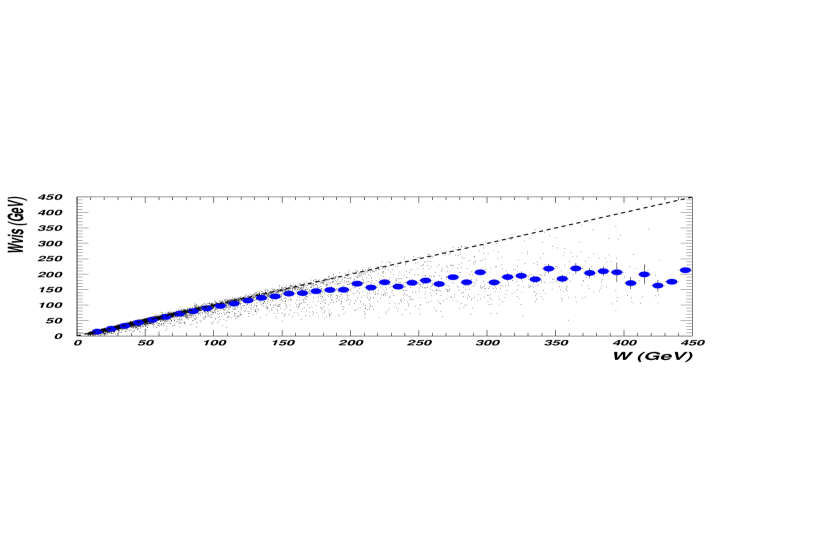
Figure 4: Comparison of $W_{\rm vis}$ with $W_{\gamma^{*}\gamma}$ from PYTHIA [19] for a typical LC detector, including the average value (profile plot).

Monte Carlo simulations of the fragmentation of the $\gamma^{*}\gamma$ system are used to correct $W_{\rm vis}$ for this loss until the uncertainty in the correction begins to dominate the measurement. Eventually, this limits the low-$x$ range of the $F_{2}^{\gamma}$ measurement.

However, if the target photon is produced by laser backscattering, two advantages are realized: 1) the high $W_{\gamma^{*}\gamma}$ (low-$x$) region is enhanced since the real photon energy is high; and 2) the energy spread of the real photons is small enough that the error on $x$ caused by assuming a monochromatic photon does not dominate the systematics.

Figure 5 shows $F_{2}^{\gamma}$ versus $Q^{2}$ for various $x$ bins from possible measurements at a future $e^{+}e^{-}$ linear collider [20]. The various points are differentiated according to the measurement method. The open squares represent the very low-$x$ region accessible only with photons produced by laser backscattering; open circles represent measurements with target photons from bremsstrahlung and with hadronic calorimetry built into a shielding mask down to $30$ mrad; solid dots represent measurements with bremsstrahlung photons and with hadronic calorimetry only outside the mask. Note that there is enough overlap between the methods to provide cross-checks on the various measurements and experimental conditions.

Figure 5: $F_{2}^{\gamma}/\alpha$ versus $Q^{2}$ in $x$ bins. Open squares: real photon target from laser backscattering; open circles: almost-real photon target from bremsstrahlung with small-angle hadronic calorimetry; solid dots: almost-real photon target from bremsstrahlung with hadronic calorimetry outside mask.

With known polarization of both the target photon and the tagged virtual photon, polarized photon structure functions can be measured for the first time. The ‘BFKL’ terms involving $\ln(1/x)$ in the unpolarized structure functions enter in polarized scattering as $\ln^{2}(1/x)$. These effects are then enhanced at low $x$ over the unpolarized case. Thus, in polarized $e\gamma$ DIS, forward particle and jet measurements, such as have been performed at HERA [21], can be done at a future $e^{+}e^{-}$ linear collider with increased sensitivity to any BFKL effects.

In addition to the $F_{2}^{\gamma}$ structure function, $e\gamma$ DIS can be used to test QCD in other ways. For example, dijet production in DIS can be used to extract the strong coupling parameter, $\alpha_{s}$, as is done at HERA [22]. At a future $e^{+}e^{-}$ linear collider, $\alpha_{s}$ from $e^{+}e^{-}$ event shapes and from dijets in DIS can be compared using the same detector.

4 $\gamma\gamma$ scattering—total cross section

Various models have been developed to describe the rise with energy of the total $\gamma\gamma$ cross section. These give either a fast rise driven by QCD effects such as minijets, or a slower rise based on reggeon exchange. To get to the highest $\sqrt{s}$ and $W_{\gamma\gamma}$, real photons from the laser backscattering process are required. Studies show that a precision of $\sim 20\%$ on the total cross section will enable adequate discrimination of model types for energies up to $1$ TeV [23]. Figure 6 shows possible $\sigma_{\rm tot}$ measurements at a 500 GeV linear collider (large stars) compared to existing measurements at lower $\sqrt{s}$ and to various models.

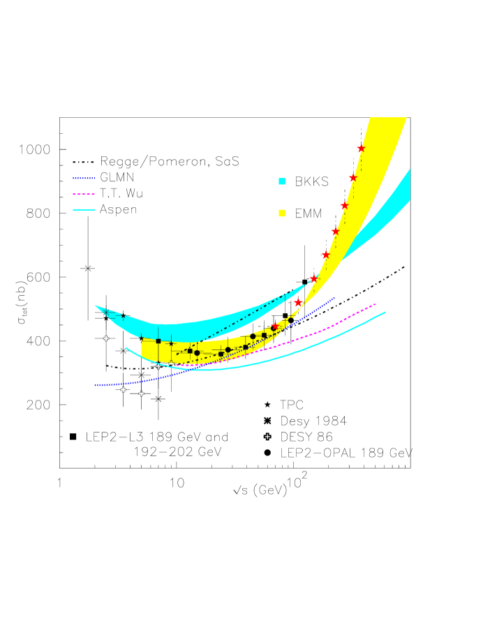
Figure 6: $\sigma_{\rm tot}$ versus $\sqrt{s}$ at a LC (large stars) compared to existing data and various models.

Using dijets from $\gamma\gamma$ scattering, the relative quark/gluon structure of the photon can be determined. Interactions between the almost-real photons produced by bremsstrahlung are determined primarily by interacting gluons in the ratio of approximately $70\%$ gluons to $30\%$ quarks. At higher $\sqrt{s}$, the gluon component should be more predominant. Thus, if real photons from laser backscattering are used, we expect to find an almost pure gluon-constituted photon ($90\%g/10\%q$) [24].

5 $\gamma^{*}\gamma^{*}$ scattering—QCD dynamics

Double-tagged virtual photon scattering completes the study of the photon at the linear collider by allowing the evolution of photon structure to be studied in an almost background-free environment. The $Q^{2}$ of each of the scattered leptons (denoted $Q_{1}^{2}$ and $Q_{2}^{2}$) is measured in the forward electromagnetic tagging calorimeters. By requiring the ratio $Q_{1}^{2}/Q_{2}^{2}\sim 1$, production of hadrons in the region between the two virtual photons through traditional DGLAP evolution is suppressed. This suppression grows stronger as the rapidity separation, $Y$, between the two virtual photons increases. At large values of $Y$, any signal above the small DGLAP background points to alternative forms of structure function evolution, e.g., to the $\ln(1/x)$ evolution of BFKL [25]. Virtual photon scattering at a linear collider provides perhaps the cleanest environment in which to study BFKL physics [26, 27].

With total center-of-mass energy $\sqrt{s}$ and photon virtuality $Q^{2}$, BFKL effects are expected in the kinematic region where the square of the photon-photon invariant mass (or, equivalently, the hadronic final-state system) is large, and

$$s\gg Q^{2}\gg\Lambda_{QCD}^{2}.$$

At fixed order in QCD, the dominant process is four-quark production with $t$-channel gluon exchange. Each photon couples to a quark box, and the quark boxes are connected via the gluon. The corresponding BFKL contribution arises from diagrams in which the $t$-channel gluon becomes a gluon ladder. At lepton-hadron or hadron-hadron colliders, the presence of hadrons in the initial state can complicate or even mask BFKL effects.

The largest values of $Y$ are obtained at low $Q_{1,2}^{2}$, again emphasizing the need for the electromagnetic tagging calorimeters to be positioned as close to the beampipe as possible. Figure 7 shows the substantially greater reach in $Y$ available to the 500 GeV LC relative to that of LEP2 running at $189$ GeV.

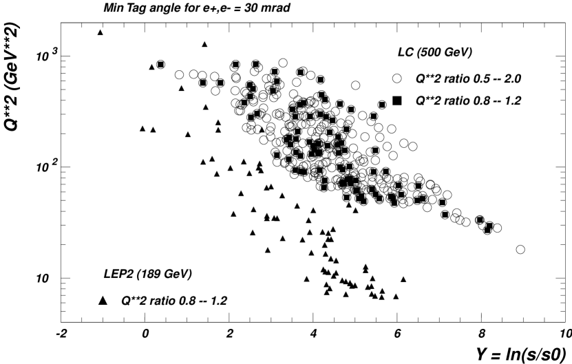
Figure 7: $Q^{2}$ versus $Y$ for a 500 GeV LC compared to LEP2.

Experiments at LEP have looked for BFKL effects in virtual photon scattering [28]. The data tend to lie between the predictions of fixed-order QCD and analytic solutions to the BFKL equation (asymptotic full-order QCD). However, the data were compared to the asymptotic QCD prediction in a non-asymptotic regime [29], so the disagreement with QCD is not surprising. In contrast, a linear collider will be expected to reach closer to the asymptotic regime, providing a more definitive test of BFKL evolution. Improved predictions are also on the way with the development of BFKL Monte Carlo programs that incorporate kinematic constraints, such as [30]. On the more theoretical front, next-to-leading log corrections have been calculated and found to be large, but the source of the large corrections is understood and they are being brought under control; see [31] for a review and references.

6 Summary of two-photon physics

The study of two-photon physics from $e^{+}e^{-}$ collisions has grown tremendously in the past several years of higher-energy LEP2 running and will continue to provide a wealth of precision measurements at a future $e^{+}e^{-}$ linear collider. Using combinations of tagged and untagged bremsstrahlung photons, aspects of real and virtual photon structure will be addressed, especially $F_{2}^{\gamma}$ at high $Q^{2}$, the relative quark/gluon content of the photon from dijets, and possible BFKL effects in QCD evolution.

With laser-backscattered real photons, the highest energies available at the linear collider can be fully exploited. $F_{2}^{\gamma}$ can be measured at very low $x$, which in combination with high $Q^{2}$ measurements from bremsstrahlung photons, will map out a kinematic region in photon structure as extensive as that known for the proton. The total $\gamma\gamma$ cross section will also be measured at the highest $\sqrt{s}$ available at the linear collider, leading to understanding of the dominant mechanisms responsible for this interaction.

Finally, with combinations of lepton and photon polarization, BFKL effects can be enhanced and the first measurements of polarized structure functions of the photon can be made.

4 Overall summary and conclusions

The high-energy linear collider offers a unique program of QCD and related two-photon studies. The strong coupling constant $\alpha_{s}$ can be measured at high $Q^{2}$ to a precision approaching $\pm 1\%$, free of the initial-state ambiguities that make the corresponding determination at a hadron collider substantially less precise, and allowing for substantial improvements in the determination of the running of the QCD coupling strength, as well as its extrapolation to the GUT scale. Constraints on the strong coupling properties of the top, providing sensitivity to a number of new physics scenarios inspired by the large mass of the top quark, can be made as much as an order of magnitude more stringent at an $e^{+}e^{-}$ collider than at a proton collider of equivalent reach.

In two-photon reactions, the precisely defined state of the incoming electron and positron beams permits the kinematic properties of the interacting virtual and nearly on-shell photons to be inferred from the properties of the recoiling electrons. This in turn allows for a unique program of photon structure and strong-force dynamics which cannot be emulated by any other proposed facility. In addition, the possibility of precisely controlled real photon beams from the Compton backscattering of polarized laser light opens up further vistas in the exploration of photon structure, and may allow the resolution of long-standing questions regarding the energy evolution of the photon-photon total cross section. Again, these studies are only possible within the larger context of an $e^{+}e^{-}$ linear collider program.

Together, these physics topics present a unique and compelling program of strong-interaction studies at a high-energy linear collider, one that adds substantial weight to the promise of the proposed linear collider physics program.

Chapter 8 Precision Studies at the $Z$ and the $WW$ Threshold

A high-precision program of electroweak and heavy-quark physics provides a natural complement to the direct searches for the Higgs boson and other new particles. The study of loop corrections to the electroweak parameters measured at the $Z$, in $p\overline{p}$ collisions and in neutrino experiments made impressive indirect predictions for the top quark mass, and constrains the mass range for a Standard Model Higgs. Limits on ${\cal B}(B\to X_{s}\gamma)$ provide the tightest mass limits on type II Higgs doublets. Because the new particles appear virtually in loops, the sensitivity extends over a much higher mass range than can be obtained in direct searches, though generally at the expense of some model–dependence.

While the physics program at 500 GeV has the potential to be very rich, it is also possible that at this center-of-mass energy there is only one Higgs-like particle seen, or no such particle at all. Under either scenario, the constraints from the electroweak and heavy-quark studies can be powerful. In the case that we do see a plethora of new particles, the full spectrum of states predicted by any model must satisfy the rules dictated by the precision measurements. In the case that very little is seen directly, the precision low-energy measurements have a good chance of showing deviations from the Standard Model. These deviations will indicate the direction that future studies must take.

There remain open issues with respect to implementing a low-energy program at a linear collider. If only the basic electroweak program is undertaken, the goals may be met by devoting a modest amount of running time at low energy. A single facility for both the high-energy and the $Z$ running, however, requires incorporation of this capability into the design of the accelerator. For a broader program, including running at $W^{+}W^{-}$ threshold and extended running at the $Z$ pole for heavy flavor physics, a low-energy facility that can operate in parallel with the high-energy may be required.

1 Electroweak observables on the $Z$ resonance

In principle, all measurements done at LEP and SLC can be repeated at the linear collider with much higher statistics. In about 100 days of running, it is possible to collect a sample of $10^{9}$ $Z$ decays (‘Giga-Z’), about 100 times the LEP or 1000 times the SLC statistics. A high degree of electron polarization seems certain and ${\cal P}_{\rm{e}^{-}}=80\%$ will be assumed in the following. Positron polarization is desirable and the R&D to achieve it is under way. Both options, with and without positron polarization, will be discussed. The issue of positron polarization is discussed further in Chapter 12.

1 Machine issues

In the present designs, the linear collider can deliver a luminosity ${\cal L}\sim 5\times 10^{33}{\rm cm}^{-2}{\rm s}^{-1}$ at the $Z$ resonance. The energy loss due to beamstrahlung for colliding particles is around $0.05\%-0.1\%$ and the depolarization in the interaction region is negligible. By sacrificing some luminosity, beamstrahlung can be reduced substantially, for example, by a factor three for a luminosity loss of a factor two [1].

Apart from the beamstrahlung there are several other effects that influence the precision of the measurements:

• The mean energies of the two beams have to be measured very precisely. A precision of $10^{-5}$ relative to the $Z$ mass might be needed to relate $A_{LR}$ to $\sin^{2}\theta_{w}^{\mathrm{eff}}$ with the desired precision.

• The beam energy spread of the machine plays a crucial role in the measurement of the total width of the $Z$. If the shape of the distribution is known, the width can be measured from the acolinearity of Bhabha events in the forward region as long as the energies of the two colliding particles are not strongly correlated.

• With the high luminosities planned, the $Z$ multiplicity in a train becomes high. This can influence $Z$ flavor tagging or even $Z$ counting.

• With positron polarization, the positron source must be able to switch polarizations on a time scale commensurate with the stability of the beam conditions.

The two main designs, X-band and superconducting, differ in some aspects relevant for $Z$ running. For the X-band design a bunch train contains 190 bunches with 1.4 ns bunch spacing, for which over half of the $Z$ bosons are produced in the same train as at least one other $Z$. Typical event separation is about 150 ns, but the experimental consequences merit some study. A TESLA bunch contains 2800 bunches with 280 ns bunch spacing. In this case bunch separation is not a problem, but data acquisition system requirements are higher. The smaller wakefields in the superconducting machine should reduce the beam energy spread. The larger bunch spacing may allow sufficient time for energy feedback, resulting in a smaller energy difference between the bunches in a train.

The LC design must accommodate the needs of the precision electroweak program in advance for the program to be viable. Suitable space in the beam delivery system for precise beam energy measurement and for polarimetry must be provided, or the beam energy measurement must be directly incorporated into the Final Focus magnet system. A measurement of these quantities behind the IP is also desirable, though it is difficult. A nonzero crossing angle might be needed.

2 Electroweak observables

There are three classes of electroweak observables that can be measured during $Z$-running at a linear collider:

• observables related to the partial widths of the $Z$, measured in a $Z$ resonance scan;

• observables sensitive to the effective weak mixing angle;

• observables using quark flavor tagging.

Table 1 summarizes the present precision and the expectations for the linear collider for these quantities.

	LEP/SLC/Tev [2]	LC
$\sin^{2}\theta_{w}^{\mathrm{eff}}$	$0.23146\pm 0.00017$	$\pm 0.000013$
lineshape observables:
$m_{Z}$	$91.1875\pm 0.0021{\rm\,GeV}$	$\pm 0.0021{\rm\,GeV}$
$\alpha_{s}(m_{Z}^{2})$	$0.1183\pm 0.0027$	$\pm 0.0009$
$\Delta\rho_{\ell}$	$(0.55\pm 0.10)\times 10^{-2}$	$\pm 0.05\times 10^{-2}$
$N_{\nu}$	$2.984\pm 0.008$	$\pm 0.004$
heavy flavors:
${\cal A}_{b}$	$0.898\pm 0.015$	$\pm 0.001$
$R_{b}^{0}$	$0.21653\pm 0.00069$	$\pm 0.00014$

Table 1: Possible improvement in the electroweak physics quantities for $10^{9}$ $Z$’s collected at a linear collider. $N_{\nu}=3$ is assumed for $\alpha_{s}$ and $\Delta\rho_{\ell}$.

Observables from the $Z$ resonance line scan

From a scan of the $Z$ resonance curve the following quantities are measured:

• the mass of the $Z$ ($m_{Z}$);

• the total width of the $Z$ ($\Gamma_{Z}$);

• the hadronic pole cross section ($\sigma_{0}=(12\pi/m_{Z}^{2})\cdot(\Gamma_{e}\Gamma_{\mathrm{had}}/\Gamma_{Z}^{2})$);

• the ratio of the hadronic to the leptonic width of the $Z$ ($R_{\ell}=\frac{\Gamma_{\mathrm{had}}}{\Gamma_{l}}$).

From these parameters, two interesting physics quantities can be derived: the radiative correction parameter $\Delta\rho_{\ell}$ that normalizes the $Z$ leptonic width, and the strong coupling constant $\alpha_{s}$.

The LEP measurements are already systematics-limited, so statistical improvement is not the issue. From LEP, $m_{Z}$ is known to $2\times 10^{-5}$, and the other three parameters are all known to $10^{-3}$. To improve on $\alpha_{s}$ and especially on $\Delta\rho_{\ell}$, all three measured parameters must be improved. This requires one to understand the beam energy and the beam energy spread for $\Gamma_{Z}$, the hadronic and leptonic selection efficiencies for $R_{\ell}$, and the absolute luminosity for $\sigma_{0}$. With the better detectors and the higher statistics available for cross checks, the errors on the selection efficiency and on the luminosity might be improved by a factor of three relative to the best LEP experiment [3]. It is not clear whether the theory error on the luminosity can be improved beyond its present value of $0.05\%$. These errors would improve the precision on $R_{\ell}$ by a factor of four and that on $\sigma_{0}$ by 30%.

With a Møller spectrometer, one could possibly obtain a precision of $10^{-5}$ in the beam energy relative to $m_{Z}$. This would give a potential improvement of a factor of two in $\Gamma_{Z}$. However, because the second derivative of a Breit-Wigner curve at the maximum is rather large, $\Gamma_{Z}$ and $\sigma_{0}$ are significantly modified by beamstrahlung and beam energy spread. For illustration, the fitted $\Gamma_{Z}$ is increased by about $60{\rm\,MeV}$ and $\sigma_{0}$ is decreased by 1.8% for the TESLA parameters. The energy spread dominates the effect, so this particularly needs to be understood to about 2% to avoid limiting the precision on $\Gamma_{Z}$ and $\Delta\rho_{\ell}$. There is a potential to achieve this precision with the acolinearity measurement of Bhabha events [4] or to extend the scan to five scan points and fit for the energy spread, but both options need further study.

The effective weak mixing angle

If polarized beams are available, the most sensitive quantity by far to the weak mixing angle is the left-right asymmetry:

$$A_{LR} = \frac{1}{{\cal P}}\frac{\sigma_{L}-\sigma_{R}}{\sigma_{L}+\sigma_{R}}$$

$$= {\cal A}_{e}$$

$$= \frac{2v_{e}a_{e}}{v_{e}^{2}+a_{e}^{2}}$$

$${v_{e}}/{a_{e}} = 1-4\sin^{2}\theta_{w}^{\mathrm{eff}}.$$ (1)

$A_{LR}$ is independent of the final state.

The $A_{LR}$ measurement has been analyzed for the linear collider environment in [5, 1]. With $10^{9}$ $Z$’s, an electron polarization of 80% and no positron polarization, the statistical error is $\Delta A_{LR}=4\times 10^{-5}$. The error from the polarization measurement is $\Delta A_{LR}/A_{LR}=\Delta{\cal P}/{\cal P}$. At SLC, $\Delta{\cal P}/{\cal P}=0.5\%$ has been reached [6]. With some optimism a factor two improvement in $\Delta{\cal P}/{\cal P}$ is possible [1]. In combination with the improved statistics, this leads to $\Delta A_{LR}=3.8\times 10^{-4}$. This precision is already more than a factor of five improvement over the final SLD result for $\sin^{2}\theta_{w}^{\mathrm{eff}}$ and almost a factor of four over the combined LEP/SLD average.

If positron polarization is available, there is the potential to go much further using the ‘Blondel scheme’ [7]. This method of polarization measurement, and the associated techniques for obtaining polarized positrons, are described in more detail in Chapter 12. To summarize the results, the total cross section with both beams polarized is given as $\sigma\,=\,\sigma_{u}\left[1-{\cal P}_{\rm{e}^{+}}{\cal P}_{\rm{e}^{-}}+A_{LR}({\cal P}_{\rm{e}^{+}}-{\cal P}_{\rm{e}^{-}})\right]$, where $\sigma_{u}$ is the unpolarized cross section. If all four helicity combinations are measured, $A_{LR}$ can be determined without polarization measurement as

$$A_{LR}\,=\,\sqrt{\frac{(\sigma_{++}+\sigma_{-+}-\sigma_{+-}-\sigma_{--})(-\sigma_{++}+\sigma_{-+}-\sigma_{+-}+\sigma_{--})}{(\sigma_{++}+\sigma_{-+}+\sigma_{+-}+\sigma_{--})(-\sigma_{++}+\sigma_{-+}+\sigma_{+-}-\sigma_{--})}}\ .$$

Figure 1 shows the error on $A_{LR}$ as a function of the positron polarization. For ${\cal P}_{\rm{e}^{+}}>50\%$ the dependence is relatively weak. For $10^{9}$ $Z$’s, the Blondel scheme with a positron polarization of 20% gives a better result than a polarization measurement of $0.1\%$ and electron polarization only.

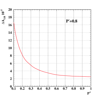
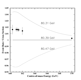
Figure 1: Left: Error of $A_{LR}$ as a function of the positron polarization for a luminosity corresponding to $10^{9}$ unpolarized $Z$’s. The errors assume that switching of the positron polarization can be done on a time scale over which the beam conditions are suitably stable. Right: The ratio of the measured $W^{+}W^{-}$ cross section to the predicted cross section for $M_{W}=80.39$ GeV (see Section 2). The data were generated using $M_{W}=80.36$ GeV. The upper (lower) curves show the ratio of the predicted cross section for $M_{W}=80.31$ GeV ($M_{W}=80.47$ GeV) to that for $M_{W}=80.39$ GeV.

Polarimeters are still needed to resolve one remaining question. There could potentially be a difference between the absolute values of the polarization in the left- and right-handed states. If the two polarization values for electrons and positrons are written as ${\cal P}_{\rm{e}^{\pm}}=\pm|{\cal P}_{\rm{e}^{\pm}}|+\delta{\cal P}_{\rm{e}^{\pm}}$, the dependence on this difference is $\rm{d}A_{LR}/\rm{d}\delta{\cal P}_{\rm{e}^{\pm}}\approx 0.5$. One therefore needs to understand $\delta{\cal P}_{\rm{e}^{\pm}}$ to $<10^{-4}$. If polarimeters with at least two channels are available, $\delta P$ can be measured together with other systematic effects intrinsic to the polarimeters in a way that does not increase the statistical error from the Blondel scheme.

Because of $\gamma$–$Z$ interference, the dependence of $A_{LR}$ on the beam energy is $\rm{d}A_{LR}/\rm{d}\sqrt{s}$ $=2\times 10^{-2}/{\rm\,GeV}$. The difference $\sqrt{s}-m_{Z}$ thus needs to be known to about $10{\rm\,MeV}$ to match the measurement with electron polarization only, and to about $1{\rm\,MeV}$ if polarized positrons are available. For the same reason beamstrahlung shifts $A_{LR}$. The shift is $9\times 10^{-4}$ for TESLA and is larger for NLC/JLC [1]. The uncertainty can only be a few percent. If beamstrahlung in the $A_{LR}$ running is identical to that in the $Z$ scan used to calibrate the beam energy, the effect is absorbed into the mean energy measured in the calibration. In that case, practically no correction would be needed for $A_{LR}$. How well the beam parameters can be kept constant during the scan and how well the beamstrahlung can be measured still need further study. However, for $A_{LR}$, only the beamstrahlung and not the energy spread matters. If the beamstrahlung cannot be understood to the required level in the normal running mode one can still go to a mode with lower beamstrahlung at the expense of lower luminosity. The cost is an increase in the statistical error or the running time.

Finally, the rate at which the positron polarization must be switched, and the switching rates that are achievable are still unknown.

For the interpretation of the data it will be assumed that $\Delta A_{LR}=10^{-4}$ is possible. This leads to $\Delta\sin^{2}\theta_{w}^{\mathrm{eff}}=0.000013$. It must be kept in mind that this error will increase by a factor of four if no positron polarization is available.

Observables with tagged quarks

By the use of quark tagging in addition to the observables discussed above, the partial widths and forward-backward asymmetries for $b$ and $c$ quarks can be measured. These observables are sensitive to vertex corrections at the $Zqq$ vertex and to new Born-level effects that alter the SM relations between quarks and leptons. The $Zbb$ vertex is particularly interesting, since the $b$ is the partner of the heavy top quark, and since the vertex corrections are naturally enhanced with the quark mass.

To date, only the improvement to the $b$-quark observables has been estimated [5]. For the ratio $R_{b}$ of the $Z$ partial widths to $b$ quarks and to hadrons, an improvement of a factor five to the LEP/SLD average is possible. This improvement is due to the much better $b$ tagging than at LEP. The improved tagging results in a higher purity (over 99% for a 30% efficiency) and a smaller energy dependence, which in turn reduces the hemisphere correlations.

The forward-backward asymmetry with unpolarized beams measures the product of the coupling parameters for the initial-state electrons and the final-state quarks: $A_{\rm FB}^{q}=\frac{3}{4}{\cal A}_{e}{\cal A}_{q}$, while the left-right forward-backward asymmetry with polarized beams measures the quark couplings directly: $A_{\rm LR,FB}^{q}=\frac{3}{4}{\cal P}{\cal A}_{q}$. For this reason a factor 15 improvement on ${\cal A}_{b}$ relative to the LEP/SLC result is possible if polarized positrons are available, and if other systematic effects are relatively small. With polarized electrons only, the improvement is limited by the polarization error to a factor of six. For control of systematics, the improved $b$-tagging capabilities are essential here as well.

Though the SM predicts that $Z$ decays to quarks are flavor-diagonal to a very good approximation, loop effects of new physics can induce flavor-violating rare decays [8]. These could be searched for at a high-luminosity $Z$ factory. For $Z\to b\overline{s}$ decays, the SM predicts a branching ratio of ${\cal{B}}(Z\to b\overline{s})\simeq 1.4\cdot 10^{-8}$. To date, the direct experimental bound on this process is relatively weak, at the level of about $10^{-3}$ [9], though bounds from rare $b$ decays such as $b\to s\ell^{+}\ell^{-}$ and $b\to s\nu\overline{\nu}$ lead to a bound ${\cal{B}}(Z\to b\overline{s})\mathrel{\raise 1.29167pt\hbox{$<$\kern-7.5pt\lower 4.30554pt\hbox{$\sim$}}}5\cdot 10^{-7}$ [8]. Still, there is room for a new physics contribution that might be revealed in a large sample of $Z$ decays.

2 $m_{W}$ from $WW$ threshold running

The mass $m_{W}$ of the $W$ boson plays a fundamental role in constraints on the Standard Model via comparison of direct measurement with the prediction based on other electroweak parameters. The electroweak measurements from LEP1 and Giga-Z—combined with the Higgs boson and top quark mass measurements from the linear collider—allow $m_{W}$ to be predicted to about 3 MeV within the SM. Measurements at the Tevatron and at LEP2 combine to give an $m_{W}$ precision of 34 MeV [10]. The LEP2 experiments hope to reach a combined precision of 35 MeV. With Run II at the Tevatron, 30 MeV per experiment appears feasible with 2 $\textrm{fb}^{-1}$, though systematics, correlated between experiments, will dominate [11]. The LHC experiments hope to reach an uncertainty of 20 MeV each, for perhaps an overall uncertainty of 15 MeV [12]. Unfortunately, these uncertainties remain significantly larger than that expected for the indirect determination and would limit the power of the electroweak constraints.

A high-luminosity linear collider presents an opportunity to measure $m_{W}$ with a much higher precision. The two potential approaches [13] are a $W^{+}W^{-}$ threshold scan and kinematic fitting of events with $W^{+}W^{-}$ production. With expected linear collider luminosities, one could obtain 100 fb^-1 in one year ($10^{7}$ s) at $W^{+}W^{-}$ threshold and about 1000 fb^-1 at $\sqrt{s}=500$ GeV in several years. The threshold scan requires precise determination of the absolute average beam energy and of the distortion of the luminosity spectrum by beamstrahlung. The kinematic fitting method also requires precise knowledge of the beam energy, since it relies on a beam energy constraint. The uncertainty from this parameter will grow with energy, since beam calibration will likely refer back to the $Z$ peak. Furthermore, the energy spread from beamstrahlung grows approximately as the square of the beam energy.

The four-quark ($4q$) channel (46% of the rate) cannot be used in the kinematic analysis because of theoretical uncertainties associated with final-state interactions between the decay products of the $W^{+}$ and the $W^{-}$. This uncertainty contributes an error of 40–90 MeV for the current LEP $4q$ measurements [14, 15, 16, 17]. Scaling of the LEP2 statistical precision for the remaining channels results in a 5 MeV $m_{W}$ precision at 500 GeV. However, significant reductions in systematics will be needed. In particular, the difficulties in beam energy calibration disfavor the direct reconstruction method.

1 $m_{W}$ from a polarized threshold scan

The extraction of $m_{W}$ from a threshold scan requires an accurate theoretical description of the cross-section dependence on $m_{W}$. The main corrections to the Born approximation near threshold come from QED. Fortunately, the dominant Coulomb correction (about 6%) is already known to all orders [18]. To keep the theoretical uncertainty down to 2 MeV, however, the electroweak and QCD corrections to the cross section must be known to 0.12% (about the size of the second-order Coulomb contribution). While work is needed, this goal appears attainable.

Recent studies [19, 20] indicate that experimental systematics can be controlled to obtain a 5 MeV $m_{W}$ measurement with 100 fb^-1of data if a polarization of 60% for the positron beam can be achieved. The strategy capitalizes on the domination of the $W^{+}W^{-}$ cross section near threshold by the $t$–channel $\nu_{e}$ exchange process, which couples only to the $e_{R}^{+}e_{L}^{-}$ helicity combination. The correct $e_{R}^{+}e_{L}^{-}$ beam polarization enhances $W^{+}W^{-}$ production relative to the background, while the $e_{L}^{+}e_{R}^{-}$ polarization has almost negligible $W^{+}W^{-}$ production and so can constrain the background levels.

A sample scan is illustrated in Fig. 1. This study assumes that the absolute luminosity and the reconstruction efficiencies can be determined with a relative (pointto-point) accuracy of 0.25%. This is four times looser than that achieved for the LEP1 $Z$ line-shape scan. Beam polarizations are assumed known to 0.25%, and are further constrained at each scan point by exploring various polarization combinations. About 90% of the luminosity is given to the main $e_{R}^{+}e_{L}^{-}$ to $e_{R}^{+}e_{L}^{-}$ configurations, in a 5:1 ratio, with the 10% devoted to the remaining configurations to determine the beam polarization. LEP signal efficiencies and background rates [21] are assumed; this should be conservative for a linear collider detector. The $W$ width $\Gamma_{W}$ is assumed to have the SM value. Under these assumptions, a precision on $m_{W}$ of 4.9 MeV is predicted for 100 fb^-1of data.

To reduce the dependence of the $m_{W}$ precision on the absolute beam polarization determination, ‘radiative return’ ($e^{+}e^{-}\to\gamma+Z$) events can be incorporated into the analysis. They are sufficiently numerous—$10^{7}$ in 100 fb^-1—that the Blondel scheme described in the previous section can be employed to measure the polarization. After fine tuning of the luminosity distribution among various helicity configurations, a scan can still determine $m_{W}$ to 5 MeV without the 0.25% polarization calibration.

The background from $e^{+}e^{-}\to q\overline{q}$ and its polarization asymmetry is neglected in this analysis. It is possible that the polarization asymmetry of the sample of background events that pass the $WW$ event selection cuts will be poorly known. In this case, the scan strategy above may not be optimal for control of the systematics. While further study is warranted, incorporation of a scan point below threshold should control the uncertainties without significantly degrading precision on $m_{W}$.

The beam-energy and beamstrahlung uncertainties of a $W^{+}W^{-}$ threshold scan must be controlled to a few MeV to achieve the desired $m_{W}$ precision. One method [22] provides a direct measurement of the average $\sqrt{s}$ via reconstruction of $e^{+}e^{-}\to\gamma+Z$, $Z\to e^{+}e^{-}/\mu^{+}\mu^{-}$. This measurement includes the average beamstrahlung effect. A precision of 2.5 MeV may be possible for 100 fb^-1. Absolute alignment of the detector polar angle to $10^{-5}$ and knowledge of the radiative corrections will be needed. One could also calibrate a precise beam spectrometer using the $Z$ line shape and extrapolate to the $W^{+}W^{-}$ threshold. The uncertainty from the LEP1 $m_{Z}$ measurement will cancel in the $m_{W}/m_{Z}$ ratio. Beamstrahlung both reduces the effective $W^{+}W^{-}$ cross section at threshold and distorts the shape. To limit the effects to 2 MeV, the absolute induced distortion must be known to 0.1%. Mapping of the distortion to this accuracy appears feasible by measurement of the distribution in the acolinearity angle in Bhabha scattering at forward angles [23]. All of these aspects of the precision energy determination will be challenging if one wishes to achieve a 2 MeV error from this source.

2 Conclusion

The experimental systematics for an $m_{W}$ measurement near $W^{+}W^{-}$ threshold appear to be under control at the few-MeV level. Issues related to beam energy and beamstrahlung deserve further attention, but cautious optimism is appropriate. Certainly the $m_{W}$ issues should be considered in the accelerator and interaction region design. Given the one year of running required to reach the order 5 MeV accuracy in $m_{W}$, consideration of a dedicated low-energy facility seems appropriate. The feasibility of the measurement without positron polarization needs examination. A much longer running period would be necessary just to make up the loss in $W^{+}W^{-}$ production. The impact on control of the background level is currently unknown.

3 Electroweak tests of the Standard Model

The physics program outlined above opens new opportunities for high-precision physics in the electroweak sector. For reference, Table 2 [24] summarizes the present and anticipated precisions for the most relevant electroweak observables at the Tevatron—Run II (2 fb^-1) and TeV33 (30 fb^-1), the LHC, and a future linear collider without (LC) and with (Giga-Z) a low-energy program.

	now	Run II		TeV33		LHC		LC		Giga-Z
$\delta\sin^{2}\theta_{w}^{\mathrm{eff}}(\times 10^{5})$	17	50	[28]	13	[28]	21	[28, 30]	(6)	[28]	1.3	[5]
$\delta m_{W}$ [MeV]	37	30	[11]	15	[12]	15	[12, 30]	15	[32]	6	[34]
$\delta m_{t}$ [GeV]	5.1	4.0	[28]	2.0	[28]	2.0	[28, 31]	0.2	[33]	0.2
$\delta m_{h}$ [MeV]	—	—		2000	[29]	100	[29]	50	[29]	50	[29]

Table 2: The expected experimental precision from various collider programs for $\sin^{2}\theta_{w}^{\mathrm{eff}}$, $m_{W}$, $m_{t}$ and the Higgs boson mass, $m_{h}$, assuming $m_{h}=110{\rm\,GeV}$. For the LC entry in parentheses, a fixed-target polarized Møller scattering experiment using the $e^{-}$ beam has been assumed. The present uncertainty on $m_{W}$ will be improved with the final analysis of the LEP2 data.

The SM predictions for the electroweak precision observables are affected via loop corrections by contributions from the top quark mass, $m_{t}$, and the Higgs boson mass, $m_{h}$. The prediction for the $W$ boson mass is obtained from

$$m_{W}=\frac{m_{Z}}{\sqrt{2}}\,\sqrt{1+\sqrt{\frac{4\,\pi\,\alpha}{\sqrt{2}\,G_{F}\,m_{Z}^{2}}(1+\Delta r)}},$$ (2)

where the loop corrections are contained in $\Delta r$ [25]. Beyond one-loop order, the QCD corrections are known at ${\cal O}(\alpha\alpha_{s})$ [26] and ${\cal O}(\alpha\alpha_{s}^{2})$ [27]. The electroweak two–loop corrections have recently been extended to include the complete fermionic contribution at ${\cal O}(\alpha^{2})$ [35].

The effective leptonic weak mixing angle, $\sin^{2}\theta_{w}^{\mathrm{eff}}$, is defined through the effective couplings $g_{V}^{f}$ and $g_{A}^{f}$ of the $Z$ boson to fermions at the $Z$ resonance,

$$\sin^{2}\theta_{w}^{\mathrm{eff}}=\frac{1}{4\,Q_{f}}\left(1-\frac{\mbox{Re}\,\,g_{V}^{f}}{\mbox{Re}\,\,g_{A}^{f}}\right),$$ (3)

where the loop corrections enter through $g_{V,A}^{f}$. The radiative corrections entering the relations (2) and (3) depend quadratically on $m_{t}$, while the leading dependence on $m_{h}$ is only logarithmic.

The current theoretical uncertainties [36] are dominated by the uncertainties in the input parameters $m_{t}$ and $m_{h}$, and in the value of the running electromagnetic coupling constant evaluated at the scale $m_{Z}$. Let $\Delta\alpha=\alpha(m_{Z})-\alpha(0)$. This difference results from electromagnetic vacuum polarization corrections due to the charged leptons and light quarks. The hadronic contributions to $\Delta\alpha$ currently give rise to an uncertainty $\delta\Delta\alpha\approx\pm 2\times 10^{-4}$ [37]. If future low-energy $e^{+}e^{-}$ experiments can measure the hadronic total cross section up to the $J/\psi$ to 1%, it is possible to reduce this uncertainty to about $\delta\Delta\alpha=\pm 7\times 10^{-5}$ [38]. As an estimate for the future theoretical uncertainties in the prediction of $m_{W}$ and $\sin^{2}\theta_{w}^{\mathrm{eff}}$ from unknown higher-order corrections (including the uncertainties from $\delta\Delta\alpha$) we use

$$\delta m_{W}(\mbox{theory})=\pm 3{\rm\,MeV},\quad\delta\sin^{2}\theta_{w}^{\mathrm{eff}}(\mbox{theory})=\pm 3\times 10^{-5}\quad\mbox{(future)}.$$ (4)

The experimental error on $m_{Z}$ ($\delta m_{Z}=\pm 2.1{\rm\,MeV}$ [10]) leads to an uncertainty in $\sin^{2}\theta_{w}^{\mathrm{eff}}$ of $\delta\sin^{2}\theta_{w}^{\mathrm{eff}}=\pm 1.4\times 10^{-5}$. While this uncertainty can currently be neglected, it will have non-negligible impact given the precision obtainable at Giga-Z. The future experimental error in the top quark mass, $\delta m_{t}=\pm 130{\rm\,MeV}$, induces further uncertainties $\delta m_{W}=\pm 0.8{\rm\,MeV}$ and $\delta\sin^{2}\theta_{w}^{\mathrm{eff}}=\pm 0.4\times 10^{-5}$.

	$m_{W}$	$\sin^{2}\theta_{w}^{\mathrm{eff}}$	all
now	200%	62%	60%
Run II	77%	46%	41%
TeV33	39%	28%	26%
LHC	28%	24%	21%
LC	18%	20%	15%
Giga-Z	12%	7%	7%

Table 3: Cumulative expected precisions for the indirect determination of the Higgs boson mass, $\delta m_{h}/m_{h}$, taking into account the error projections in Table 2 and the theoretical uncertainties of $m_{W}$ and $\sin^{2}\theta_{w}^{\mathrm{eff}}$. The first two columns use $m_{W}$ and $\sin^{2}\theta_{w}^{\mathrm{eff}}$ constraints alone, while the last column uses the full set of precision observables.

Comparison of an indirect determination of the SM Higgs boson mass, which would be significantly improved by Giga-Z [39, 24, 40, 5], with a future direct measurement will provide a sensitive test of the SM. Table 3 [24] summarizes both today’s accuracy for the indirect prediction of $m_{h}$ and the accuracy available from the prospective improvements at forthcoming colliders listed in Table 2. The current accuracies assume $\delta\Delta\alpha=\pm 2\times 10^{-4}$ [37], while the future cases assume $\delta\Delta\alpha=\pm 7\times 10^{-5}$ [38]. The Giga-Z scenario allows an indirect determination of $m_{h}$ with an uncertainty of $\delta m_{h}/m_{h}=\pm 7\%$ (about the level of the current indirect $m_{t}$ determination). This represents a factor of three improvement over the EW constraints that could be made using LHC measurements, while a linear collider running solely at high energy would provide only a modest gain.

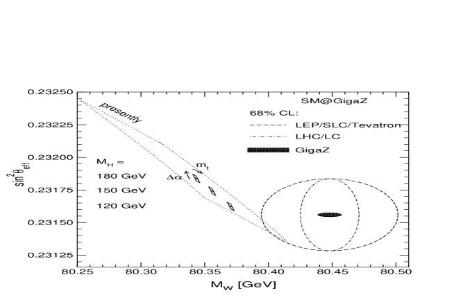
Figure 2: The present and prospective future theoretical predictions in the SM (for three $m_{h}$ values) are compared with the current experimental accuracies and those expected from LHC and Giga-Z (see Table 2). The future theoretical uncertainties arising from $\delta\Delta\alpha=\pm 7\times 10^{-5}$ and $\delta m_{t}=\pm 200{\rm\,MeV}$ are indicated.

Figure 2 compares the potential of Giga-Z for testing the electroweak theory with the present status from both theoretical and experimental standpoints. The SM prediction corresponds to an allowed $m_{h}$ interval of $113{\rm\,GeV}\leq m_{h}\leq 400{\rm\,GeV}$ and to an allowed $m_{t}$ interval within its measured uncertainty. The theoretical prediction assumes that the Higgs boson has been found, with masses of 120, 150 and 180 GeV considered. The uncertainty induced assuming $\delta m_{t}=\pm 200$ MeV and $\delta\Delta\alpha=\pm 7\times 10^{-5}$ is indicated. The figure illustrates that the improved experimental accuracy at Giga-Z will allow tests of the internal consistency of the SM at an unprecedented level.

1 Parameterizations of deviations from the Standard Model

The precision achievable at Giga-Z allows for the exploration of possible effects of new physics with great sensitivity. This section is devoted to more general parameterizations of physics beyond the SM through the specific example of the $S$, $T$, $U$ parameters [41]. While these parameters are widely used, considerable confusion exists concerning their meaning and range of applicability. Because it is important to understand precisely how the effects of new physics can be probed in a sensible way given the potential Giga-Z accuracies, we briefly summarize the main points.

By definition, the $S$, $T$, $U$ parameters describe only the effects of new physics contributions that enter via vacuum-polarization effects (i.e., self-energy corrections) to the vector-boson propagators of the SM. That is, the new physics contributions are assumed to have negligible couplings to SM fermions. The parameters can be computed in new models as certain combinations of one-loop self-energies. Experimentally, their values are determined by comparing the measurements, ${\cal A}_{i}^{\mathrm{exp}}$, of a number of observables with their SM predictions, ${\cal A}_{i}^{\mathrm{SM}}$,

$${\cal A}_{i}^{\mathrm{exp}}={\cal A}_{i}^{\mathrm{SM}}+f^{\mathrm{NP}}_{i}(S,T,U).$$ (5)

Here ${\cal A}_{i}^{\mathrm{SM}}$ contains all known radiative corrections in the SM evaluated at reference values of $m_{t}$ and $m_{h}$. The (linear) function $f^{\mathrm{NP}}_{i}(S,T,U)$ describes the contributions of new physics. For most precision observables, the corrections caused by a variation of $m_{t}$ and $m_{h}$ at one-loop order can also be absorbed into $S$, $T$, and $U$. A non-zero result for $S$, $T$, $U$ determined in this way indicates non-vanishing contributions of new physics (with respect to the SM reference value).

The $S$, $T$, $U$ parameters can only be applied for parameterizing effects of physics beyond the SM. To compute the SM predictions to which these parameters provide corrections, one must take into account the full contributions, which also contain vertex and box corrections, since these effects cannot be consistently absorbed into the $S$, $T$, $U$ parameters. For a more detailed discussion of this point, see [42]. Because the $S$, $T$, $U$ parameters are restricted to the leading-order contributions of new physics, they should only be applied for small deviations from the SM predictions. Their application to cases with large deviations from the SM, like extensions of the SM with a very heavy Higgs boson in the range of several TeV, is questionable. The current experimental values [43] (assuming $m_{t}=173.4{\rm\,GeV}$ and $m_{h}=100{\rm\,GeV}$) are

$$S=-0.07\pm 0.11,\quad T=-0.10\pm 0.14,\quad U=~{}0.10\pm 0.15.\quad$$ (6)

Other parameterizations, defined via linear combinations of various observables without reference to the SM contribution, have been suggested (see, e.g., [44, 45]). While any new physics model can be explored, it is not in all cases obvious that studying parameters is of advantage compared to studying the observables themselves. For this reason and for brevity, we restrict our discussion to the $S$, $T$, $U$ parameters.

Examples of new physics contributions that can be described in the framework of the $S$, $T$, $U$ parameters are contributions from a fourth generation of heavy fermions or effects from scalar quark loops (see Section 2). A counterexample going beyond the $S$, $T$, $U$ framework is given by corrections of the kind that could bring the prediction for the anomalous magnetic moment of the muon in agreement with the experimental value [46, 47].

While many SM extensions result in a vanishing or small contribution to the $U$ parameter (see  Ref. [43] and references therein), sizable contributions to $S$ and $T$ can be expected from a number of models. For instance, the contribution of a heavy Higgs boson with $m_{h}=1{\rm\,TeV}$ gives rise to a contribution in $S$ and $T$ of about $S\approx 0.1$, $T\approx-0.3$ [48] (see however the discussion above). In technicolor models one typically expects $S$ and $T$ to be positive and of order 1 [48]. Peskin and Wells [48] have also examined the ‘topcolor seesaw’ model of Dobrescu and Hill [49], which predicts little or no new physics observable at the LHC or LC. The Giga-Z scenario, however, would reveal a significant departure in the $(S,T)$ plane from the minimal SM with a light Higgs boson.

These additional contributions to the $S,T,U$ parameters have to be compared with the errors with which these parameters can be extracted at Giga-Z [24]:

$$\Delta S=\pm 0.05,\quad\Delta T=\pm 0.06,\quad\Delta U=\pm 0.04.\quad$$ (7)

These parameters are strongly correlated. Assuming $U=0$, as justified above, the anticipated errors in $S$ and $T$ would decrease to about

$$\Delta S=\pm 0.02,\quad\Delta T=\pm 0.02.\quad$$ (8)

The increased precision, compared to the present situation given in Eq. (6), will constrain or exclude of many possible extensions of the SM.

2 Tests of supersymmetry

We now explore the utility of the precision electroweak observables in a scenario with direct observation of new particles, by examining a specific example. Suppose that particles compatible with a MSSM Higgs boson and a light scalar top quark $\tilde{t}_{1}$ have been discovered at the Tevatron or the LHC, and further explored at an $e^{+}e^{-}$ linear collider. With the luminosity expected at a linear collider, the $\tilde{t}_{1}$ mass, $m_{\tilde{t}_{1}}$, and the mixing angle in the stop sector, $\cos\theta_{\tilde{t}}$, can be measured in the process $e^{+}e^{-}\to\tilde{t}_{1}\tilde{t}_{1}^{*}$ to a level below 1% [50, 51].

The precision electroweak variables provide several constraints. First, the measurements and predictions for $m_{W}$ and $\sin^{2}\theta_{w}^{\mathrm{eff}}$ provide an indirect test of the MSSM, as they do for the SM. Comparison of the predicted to the measured value of the lightest CP-even MSSM Higgs boson mass, $m_{h}$, provides a further constraint. In the MSSM, $m_{h}$ is not a free parameter as in the SM; it is calculable from the other SUSY parameters. Furthermore, because $m_{W}$, $\sin^{2}\theta_{w}^{\mathrm{eff}}$ and $m_{h}$ are particularly sensitive to the SUSY parameters of the scalar top and bottom sector and of the Higgs sector, they provide an indirect probe of the masses of supersymmetric particles that might not be seen at the LHC or LC. In particular, the heavier scalar top quark, $\tilde{t}_{2}$, and the heavy Higgs bosons $A$, $H$ and $H^{\pm}$ could be outside the kinematic reach of the initial-stage LC, and background problems could preclude their observation at the LHC. Reference [24] explores this scenario and demonstrates that upper bounds on $M_{A}$ could be established through the SUSY contributions to $m_{W}$ and $\sin^{2}\theta_{w}^{\mathrm{eff}}$, just as the Higgs boson mass can be bounded in the SM.

Finally, we examine the indirect information on the mass of the heavier scalar top quark, $m_{\tilde{t}_{2}}$, that can be obtained by requiring consistency of the MSSM with measurements of $m_{W}$, $\sin^{2}\theta_{w}^{\mathrm{eff}}$, and $m_{h}$ in addition to those of $m_{\tilde{t}_{1}}$ and $\cos\theta_{\tilde{t}}$. The SUSY contributions to $m_{W}$ and $\sin^{2}\theta_{w}^{\mathrm{eff}}$ include the complete one–loop results in the MSSM [52] as well as the leading higher-order QCD corrections [53]. The prediction for $m_{h}$ is obtained with the program FeynHiggs [54], based on the Feynman-diagrammatic two-loop result of Ref. [55]. A future uncertainty in the theoretical prediction of $m_{h}$ of $\pm 0.5{\rm\,GeV}$ is assumed.

We examine the scenarios for a LC with and without the Giga-Z option and for the LHC (see Table 2), taking $m_{\tilde{t}_{1}}=180\pm 1.25{\rm\,GeV}$ for LC/Giga-Z, and $180\pm 18{\rm\,GeV}$ for the LHC. The other parameters have been chosen according to the mSUGRA reference scenario 2 specified in Ref. [56], with the following accuracies: $M_{A}=257\pm 10$ GeV, $\mu=263\pm 1$ GeV, $M_{2}=150\pm 1$ GeV, $m_{\tilde{g}}=496\pm 10$ GeV. For $\tan\beta$ a lower bound of $\tan\beta>10$ has been taken. The central values for $m_{W}$ and $\sin^{2}\theta_{w}^{\mathrm{eff}}$ have been chosen in accordance with a non-zero contribution to the precision observables from SUSY loops.

As one can see in Fig. 3, the allowed parameter space in the $m_{\tilde{t}_{2}}$–$|\cos\theta_{\tilde{t}}|$ plane is significantly reduced in the Giga-Z scenario relative to the others. Using the direct information on $|\cos\theta_{\tilde{t}}|$ from Ref. [51] allows an indirect determination of $m_{\tilde{t}_{2}}$ with a precision of better than 5% in the Giga-Z case. By comparing this indirect prediction for $m_{\tilde{t}_{2}}$ with direct experimental information on the mass of this particle, the MSSM could be tested at its quantum level in a sensitive and highly non-trivial way.

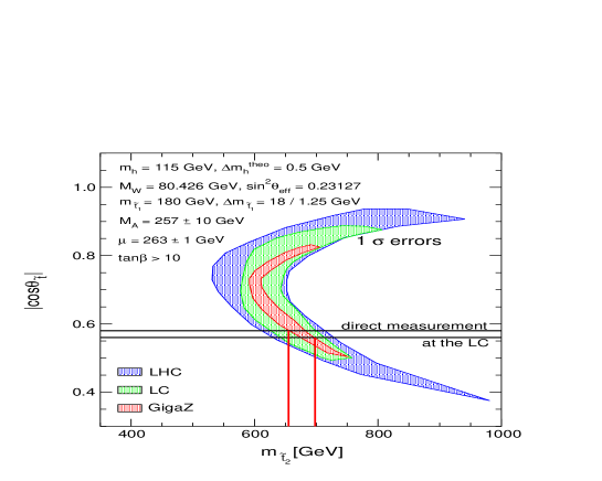
Figure 3: Indirect constraints on the MSSM parameter space in the $m_{\tilde{t}_{2}}$–$|\cos\theta_{\tilde{t}}|$ plane from measurements of $m_{h}$, $m_{W}$, $\sin^{2}\theta_{w}^{\mathrm{eff}}$, $m_{t}$ and $m_{\tilde{t}_{1}}$ at a LC with and without the Giga-Z option and at the LHC. The solid lines indicate the direct information on the mixing angle from a measurement at the LC and the corresponding indirect determination of $m_{\tilde{t}_{2}}$.

4 Heavy flavor physics

The $Z$ pole has already been established as an excellent laboratory for the study of $b$ physics. The large boost and resulting detached vertices for the $b$ decays have amply compensated the relatively modest statistics of the LEP experiments, allowing them to make many competitive and important measurements. SLD, with much smaller statistics, has benefitted greatly from the SLC’s beam polarization in the $b$ studies that require production tagging and has produced measurements competitive with LEP. The hadronic experiments, LHC-b and BTeV, will be faced with large backgrounds, with typical signal-to-noise ratios of $S/N\approx 5\times 10^{-3}$ compared to $S/N\approx 0.21$ at the $Z$ (albeit with $10^{4}$ to $10^{5}$ more $b$’s produced).

The $Z$-pole running will result in a very powerful $b$ experiment. With 80% and 60% polarizations for the electron and positron beams, respectively, production flavor tags that include the forward–backward production asymmetry should reach a signal $\times$ purity $\varepsilon D^{2}$ approaching 0.6. (With 80% electron polarization and no positron polarization, one finds about half of this value.) For comparison, the $B$ factories have achieved $\varepsilon D^{2}\approx 0.25$ [57] while the hadronic facilities will have rather lower values. Coupled with the excellent resolution expected from the vertex detector for the linear collider, a reach in $\delta m_{s}$ of $40\ \textrm{ps}^{-1}$ is possible with $10^{9}$ $Z$’s, with a resolution limit of around $80\ \textrm{ps}^{-1}$.

The scenario in which $2\times 10^{9}$ $Z$ decays are produced, yielding about $6\times 10^{8}$ $b$ hadrons, has been investigated. This sample should be compared to the $\Upsilon(4S)$ and hadronic $b$ samples that will be available in the same time period [5, 58]. This section is largely based on a review of such work in [58]. With these statistics, $b$ studies at the $Z$ offer a number of measurements that are of fundamental importance for the comprehensive $b$-physics program that is being undertaken worldwide, but which cannot be addressed adequately at other existing or planned facilities. A longer running period at the $Z$ ($10^{10}$ $Z$’s) is necessary to improve upon the sensitivity for the ‘canonical’ measurements planned at other $b$ facilities, despite the combined advantages of tagging, boost and purity. Such a facility would be quite competitive. A precision on $\sin 2\beta$ of about 0.01 would be obtainable, similar to that obtainable from LHC-b and BTeV. If one translates the studies of $B\to\pi\pi$ to an effective value of $\sin 2\alpha$, the uncertainty would be about 0.02, approaching that of BTeV and somewhat better than that expected from LHC-b.

The topics unique to a polarized $Z$ facility are the following:

1. The quark-level transition

   $$b\to q+\nu\overline{\nu}$$ (9)

   could well be affected significantly by new physics in ways quite different from $b\to q+l^{+}l^{-}$. Searching for $b\to q\nu\overline{\nu}$ in hadronic colliders appears hopeless. The searches also pose quite a challenge for an $\Upsilon(4S)$ experiment because of the intermingling of the decay productions from the two $B$ decays [59].

2. The CKM elements $|V(cb)|$ and $|V(ub)|$, determined in semileptonic $B$ decay, suffer from a potentially considerable source of uncertainty due to limitations in the validity of quark-hadron duality, of which at present little is known for certain. Detailed comparisons of semileptonic $B_{s}$ and $B_{u,d}$ decays would be invaluable in this respect. The $\Upsilon(4S)$ machines will not have $B_{s}$ samples, while the hadronic machines will have difficulty providing precise inclusive measurements.

3. The availability of polarized beams will allow production of a huge sample of highly polarized beauty baryons whose weak decays can be analyzed. In this way a determination of the handedness of a quark transition becomes feasible.

The canonical measurements for which $2\times 10^{9}$ $Z$’s may be competitive include

1. The transition $b\to\tau\nu$ contains multiple neutrinos in the final state, with an experimental situation similar to that for $b\to q+\nu\overline{\nu}$. This measurement determines the product $F_{B}|V_{ub}|$, and would play a fundamental role in constraints of the CKM matrix. The reach at Giga-Z has not yet been studied.

2. The production flavor tagging from the $Z$ running might offer the most precise measurements of ${\cal B}(B^{0}\to\pi^{0}\pi^{0})$ and ${\cal B}(\overline{B}^{0}\to\pi^{0}\pi^{0})$, which are of great significance for extracting the angle $\phi_{2}$ or $\alpha$ from the measured CP asymmetry in $B^{0}\to\pi^{+}\pi^{-}$.

The following subsections elaborate on these points.

1 Measurement prospects for ${\cal B}(B\to\pi^{0}\pi^{0})$

One of the promising strategies for measuring the CKM angle $\alpha$ is the study of the CP asymmetry in the decay $\rm B^{0}\rightarrow\pi^{+}\pi^{-}$. The presence of significant ‘penguin’ contributions to $\rm B\rightarrow\pi^{+}\pi^{-}$ complicates the extraction of $\alpha$ from the measured timedependent CP asymmetry. The penguin and tree contributions can be separated by measuring the branching ratios ${\cal B}(\rm B^{0}\rightarrow\pi^{+}\pi^{-})$, ${\cal B}(\rm B^{+}\rightarrow\pi^{+}\pi^{0})$ and ${\cal B}(\rm B^{0}\rightarrow\pi^{0}\pi^{0})$ and the charge conjugate modes [60]. The first can be measured as a by-product of the CP-asymmetry analysis, but the other two are more difficult. The need to reconstruct $\pi^{0}$s makes them extremely challenging for hadron machines. The expected branching ratios are also very small, of order $10^{-6}$, with experimental upper limits of $12.7\times 10^{-6}$ ($\pi^{+}\pi^{0}$) [61] and $9.3\times 10^{-6}$ ($\pi^{0}\pi^{0}$) [62].

The feasibility of measuring these branching ratios at a linear collider was studied [5] using the fast Monte Carlo simulation SIMDET [63]. The reconstructed $B$ mass resolutions were found to be 150 MeV ($\pi^{0}\pi^{0}$) and 120 MeV ($\pi^{+}\pi^{0}$), dominated by the calorimeter angular resolution. Assuming signal branching ratios of a few $10^{-6}$ gives signal samples of about 200 events for $2\times 10^{9}\ \rm Z^{0}$ decays, on top of several hundred events of combinatorial background. This would allow a flavor-independent measurement comparable to that of BABAR or BELLE with about $200\,\rm fb^{-1}$ [5]. For the separate $B$ versus the $\overline{B}$ branching fractions, which are needed for the $\alpha$ determination, the factor of two or more improvement in $\varepsilon D^{2}$ at the $Z$ relative to that for the $B$ factories makes these measurements with $10^{9}$ $Z$’s competitive with, if not better than, those obtainable at the $B$ factories. It should be emphasized that this study was performed with a very crude calorimeter simulation and further background rejection may certainly be possible after more detailed studies.

2 $B\to X_{q}\nu\overline{\nu}$

The large backgrounds at hadronic machines make measurement of $B\to X_{q}\nu\overline{\nu}$ impossible there. In an $e^{+}e^{-}$ threshold machine, such transitions could be found only at the cost of reconstructing one $B$ more or less fully. At Giga-Z, however, the relative cleanliness of the $Z$, the hemispheric separation of the $b$ quarks, and the well-defined initial state provide powerful tools for discovering and actually measuring properties of such transitions at the $Z$. This is illustrated by the fact that the current upper limit on this decay mode comes from LEP1:

$${\rm BR}(B\to X_{s}\nu\overline{\nu})\leq 7.7\times 10^{-4}\;\;\;{\rm(ALEPH)}\ .$$ (10)

New physics can affect $b\to ql^{+}l^{-}$ and $b\to q\nu\overline{\nu}$ in quite different way for various reasons [64]. For example, new contributions to an effective $bsZ$ vertex would enhance $b\to q\nu\overline{\nu}$ relative to $b\to ql^{+}l^{-}$ by a large factor, and study of $b\to q\nu\overline{\nu}$ (with contributions from $b\to q\nu_{\tau}\overline{\nu}_{\tau}$) in addition to $b\to qe^{+}e^{-}$ and $b\to q\mu^{+}\mu^{-}$ can help disentangle new physics scenarios with generation–dependent couplings .

At the $Z$, the statistics will be high enough to make meaningful searches for $B\to X_{s}\nu\overline{\nu}$. With an inclusive branching fraction in the standard model of about $4\times 10^{-5}$, and exclusive branching fractions to $K$ and $K^{*}$ of order $10^{-5}$ [64], one can expect a few times $10^{3}$ events in exclusive channels and about $10^{4}$ inclusively. The expected reach, including control of backgrounds such as $b\to\tau\nu$, is not known at this time, but warrants study.

3 Semileptonic $B_{s}$ decays

The CKM parameters $V_{cb}$ and $V_{ub}$ play a central role in the prediction of various CP asymmetries in $B$ and $K$ decays. With precision measurements, constraints on new physics scenarios would be obtained by comparison of the predictions with direct measurements. It is crucial for this program to have reliable determination of $V_{cb}$ and $V_{ub}$, obtained from semileptonic $B$ decays through observables in exclusive and inclusive modes.

Inclusive measurements play an important role in these determinations. The known uncertainties are estimated at the 5% level for $V_{cb}$ and at the (10–15)% level for $V_{ub}$. However, there may be an additional significant source of systematic uncertainty, the validity of quark-hadron duality, which underlies almost all applications of the $1/m_{Q}$ expansions. A large body of folkloric or circumstantial evidence suggests that duality is a useful and meaningful concept. But for a full evaluation of the data from beauty physics it is essential to know with tested confidence whether the deviations from exact duality in semileptonic transitions arise at the 10%, the 5%, or the 1% level. It is quite unlikely that this question can be answered by theoretical means alone.

Experimentally, one can probe duality via an independent extraction of $|V_{cb}|$ in $B_{s}$ decays through measurement of $\Gamma_{SL}(B_{s})$. One could also determine the rate for $B_{s}\to l\nu D^{*}_{s}$, extrapolate to zero recoil, and extract the product $|V(cb)F_{B_{s}\to D_{s}^{*}}(0)|$. The form factor can be obtained from the result of the Heavy Quark Expansion

$$|F_{B_{s}\to D_{s}^{*}}(0)|\simeq|F_{B\to D^{*}}(0)|$$ (11)

up to $SU(3)$ breaking corrections, which can be estimated.

The physical origin of duality violation would be the accidental presence of a nearby hadronic resonance with appropriate quantum numbers to affect the decay pattern for one of the $B$ mesons. On one hand, this resonance may affect $B_{d}\to l\nu X_{c}$ and $B_{u}\to l\nu X_{c}$, but not $B_{s}\to l\nu X_{c}$; conversely, it may affect $B_{s}$ transitions while having no impact on $B_{u,d}$ channels. If the same value emerged for $|V(cb)|$ in both cases, we would have verified the validity of duality in this case at least. If not, we would not know which, if any, of the values is the correct one, but we would be aware of a serious problem.

Duality violation could exhibit a different pattern in $B\to l\nu X_{u}$ channels. Here theory also calls for a detailed comparison of $B_{d}$ and $B_{u}$ modes, since one expects a difference in the endpoint region of $B_{d}$ and $B_{u}$ semileptonic decays [65]. Hadronic resonances could affect $B_{d}\to l\nu X_{u}$ and $B_{u}\to l\nu X_{u}$ quite differently. In addition, measurements of $B_{s}\to l\nu X_{u}$, both inclusive and exclusive, would provide crucial cross checks.

4 Weak decays of polarized beauty baryons

Mode	Branching Ratio	Number of Events
$\Lambda_{b}\to\Lambda_{c}\ell\overline{\nu}_{\ell}$	$8\times 10^{-2}$	$5\times 10^{6}$
$\Lambda_{b}\to p\ell\overline{\nu}_{\ell}$	$8\times 10^{-4}$	$5\times 10^{4}$
$\Lambda_{b}\to X_{s}\gamma$	$3\times 10^{-4}$	$11000$
$\Lambda_{b}\to\Lambda\gamma$	$5\times 10^{-5}$	$1400$
$\Lambda_{b}\to\Lambda\ell\ell$	$1\times 10^{-6}$	50

Table 4: Expected numbers of events for $\Lambda_{b}$ decays, based on the Standard Model estimates.

The large polarization asymmetry for $Z$ decay to $b$ quarks implies that beauty baryons produced in $Z$ decays are highly polarized. From $2\times 10^{9}$ $Z$s, one expects about $3\times 10^{7}$ polarized $b$-flavored baryons. The study of the weak decays of these particles offers a whole new field of dynamical information. The existence of initial-state polarization in $\Lambda_{b}$ decays allows one to analyze the chirality of the quark coupling directly; it also leads to a new program of studying observables revealing direct CP violation. Charmed baryons also merit study.

A generic analysis of $b\to s\gamma$ results in two transition operators, mediating the decays

$$b_{R}\to s_{L}\gamma\;,\;b_{L}\to s_{R}\gamma\;.$$ (12)

While the second operator is highly suppressed in the SM, by a factor $m_{s}/m_{b}$, these operators could be of comparable size in new physics scenarios, for example, in Left-Right Symmetric models or the MSSM. While the decays of mesons realistically cannot distinguish between these two transitions, a study of the $\Lambda$ polarization in the decay $\Lambda_{b}\to\Lambda\gamma$ with polarized $\Lambda_{b}$ could probe the SM prediction that the ratio of left- to right-handed couplings is $r\mathrel{\raise 1.29167pt\hbox{$<$\kern-7.5pt\lower 4.30554pt\hbox{$\sim$}}}0.04$. One measures the asymmetry in the angular distribution defined between the $\Lambda_{b}$ spin and the photon in the parent baryon rest frame. Based on the statistics of Table 4, corresponding to roughly 750 fully reconstructed events, the measurement would be sensitive to values of $r$ between 0.5 and 1.9 at the $5\sigma$ level. For comparison, the sensitivity extends from 0.2 and 4.1 with $10^{10}$ $Z$’s [66]. It should be noted that the angular asymmetry is a theoretically very clean observable and the extraction of $r$ is essentially limited only by statistics.

A significant non-vanishing contribution of $b_{L}\to s_{R}\gamma$ would signal the intervention of new physics. One can actually undertake an inclusive polarization study of $\Lambda_{b}\to\Lambda\gamma+X$ with large statistics; the clean environment of the $Z$ is crucial here. Corresponding studies can be performed with $\Lambda_{b}\to l^{+}l^{-}X$ with smaller statistics.

Although theoretically less clean, similar angular asymmetries in rare hadronic 2-body decays such as $\Lambda_{\rm{b}}\to\Lambda\phi$ offer a unique opportunity to probe for new physics contributions to four-quark penguin operators with chiralities opposite to those in the SM [66].

As an advantage over experiments with unpolarized $\Lambda_{b}$ baryons, spin correlations between the spin of the $\Lambda_{b}$ and the daughter baryon are fully accessible. It is possible, for example, to distinguish between pseudoscalar and vector transition form factors [67]. This allows for novel, powerful consistency checks of the Standard Model including its CP and chirality properties.

Semileptonic decays of polarized $\Lambda_{b}$ allow testing of the $V-A$ character of $b$ quarks with unprecedented accuracy and searches for CP asymmetries in the decay spectra. For example, comparison of

$$\Lambda_{b}\to l^{-}(p+X)_{\rm no\;charm}\;\;\;\textrm{vs.}\;\;\;\overline{\Lambda}_{b}\to l^{+}(\overline{p}+X)_{\rm no\;charm},$$ (13)

might reveal CP violation from new physics. In final states with at least three particles ($\Lambda_{b}\to ABC$), one can also form $T$-odd correlations such as

$$C_{T}\equiv\langle\vec{\sigma}_{\Lambda_{b}}\cdot(\vec{p}_{A}\times\vec{p}_{B})\rangle$$ (14)

with $\vec{p}_{A}$, $\vec{p}_{B}$ denoting the momenta of $A$ and $B$, respectively, and $\vec{\sigma}_{\Lambda_{b}}$ the $\Lambda_{b}$ polarization. A nonzero value of $C_{T}$ can be due either to $T$ violation or to final-state interactions. Measurement of $\overline{C}_{T}$ in the CP-conjugate process resolves the ambiguity. If $C_{T}\neq\overline{C}_{T}$, one has a signature of direct CP violation. Since these effects are typically quite suppressed in the Standard Model, such studies represent largely a search for new physics. They can be performed in nonleptonic modes

$$\Lambda^{0}_{b}\to\Lambda^{+}_{c}\pi^{-}\pi^{0},p\pi^{-}\pi^{0},\Lambda K^{+}\pi^{-}$$ (15)

as well as in semileptonic channels containing a $\tau$ lepton, since the effect is proportional to the lepton mass [68].

5 Summary

A sample of order $10^{9}$ $Z$’s will provide important and unique tools in the search for and constraint of physics beyond the Standard Model. The program available with polarized positron beams in particular provides dramatic improvement in the measurement precision of the electroweak observables at the $Z$. This improvement leads to markedly more powerful constraints on Standard Model and new physics scenarios. The polarized $b$-baryon program offers a unique window of exploration for new right–handed couplings. With the statistics and $b$-tagging capabilities available with two polarized beams, running for several years ($10^{10}$ $Z$’s) could provide a $b$ physics program rivaling the proposed hadronic experiments in some fundamental CKM measurements.

Without positron polarization, significant gains can still be made. Much of the $b$ physics would suffer only from a decrease in statistics. Impact on the $\Lambda_{b}$ asymmetry measurements needs to be evaluated. The improvement in $\Delta A_{LR}$ is still significant and useful. The most damaging aspect could be the loss of the $m_{W}$ determination from threshold running, for which it is unclear that a 5–6 MeV determination would be realistic without positron polarization. This impact still needs study.

References

- [1] K. Hagiwara, R. D. Peccei, D. Zeppenfeld and K. Hikasa, Nucl. Phys. B282, 253 (1987).
- [2] J. Bagger, S. Dawson, and G. Valencia, Nucl. Phys. B399, 264 (1993).
- [3] C. Ahn, M. E. Peskin, B. W. Lynn and S. B. Selipsky, Nucl. Phys. B309, 221 (1988); J. Fleischer, J. L. Kneur, K. Kolodziej, M. Kuroda and D. Schildknecht, Nucl. Phys. B378, 443 (1992) [Erratum-ibid. B426, 443 (1992)].
- [4] A. Arhrib, J. L. Kneur and G. Moultaka, Phys. Lett. B376, 127 (1996); E. N. Argyres, A. B. Lahanas, C. G. Papadopoulos and V. C. Spanos, Phys. Lett. B383, 63 (1996); G. Couture, J. N. Ng, J. L. Hewett, and T. G. Rizzo, Phys. Rev. D38, 860 (1988).
- [5] M. Kitahara, M. Marui, N. Oshimo, T. Saito and A. Sugamoto, Eur. Phys. J. C4, 661 (1998), [hep-ph/9710220].
-
[6]
C. Burgard, in Physics and Experiments with Future Linear Colliders,
E. Fernández and A. Pacheco, eds. (UAB Publications, Barcelona, 2000);
W. Menges, “A Study of Charge Current Triple Gauge Couplings at TESLA.” LC-PHSM-2001-022.
http://www.desy.de/~lcnotes. - [7] D. Choudhury, J. Kalinowski, Nucl. Phys. B491, 129 (1997); D. Choudhury, J. Kalinowski, A. Kulesza, Phys. Lett. B457, 193 (1999).
- [8] ATLAS Detector and Physics Performance Technical Design Report, LHCC 99-14/15 (1999).
- [9] A. Vicini, Acta Phys. Polon. B29, 2847 (1998).
- [10] M. W. Grünewald et al., in Reports of the Working Groups on Precision Calculations for LEP2 Physics, S. Jadach, G. Passarino, and R. Pittau, eds. (CERN 2000-009, Geneva, 2000) [hep-ph/0005309].
- [11] W. Beenakker, F. A. Berends and A. P. Chapovsky, Nucl. Phys. B548, 3 (1999).
- [12] A. Denner, S. Dittmaier, M. Roth and D. Wackeroth, Nucl. Phys. B587, 67 (2000); Phys. Lett. B475, 127 (2000).
- [13] S. Jadach, W. Placzek, M. Skrzypek, B. F. Ward and Z. Was, Phys. Lett. B417, 326 (1998); Phys. Rev. D61, 113010 (2000); hep-ph/0007012; hep-ph/0103163; hep-ph/0104049.
- [14] Y. Kurihara, M. Kuroda and D. Schildknecht, Nucl. Phys. B565, 49 (2000).
- [15] A. Denner, S. Dittmaier, M. Roth and D. Wackeroth, hep-ph/0104057; A. Denner, S. Dittmaier, M. Roth and D. Wackeroth, in Proceedings of the 22nd Annual MRST Meeting, C.R. Hagen, ed. (Melville, NY, 2000) [hep-ph/0007245].
- [16] W. J. Stirling and A. Werthenbach, Phys. Lett. B466, 369 (1999); Eur. Phys. J. C14, 103 (2000).
- [17] G. Belanger, F. Boudjema, Y. Kurihara, D. Perret-Gallix and A. Semenov, Eur. Phys. J. C13, 283 (2000).
- [18] P. J. Dervan, A. Signer, W. J. Stirling and A. Werthenbach, J. Phys. G26, 607 (2000).
- [19] G. Montagna, M. Moretti, O. Nicrosini, M. Osmo and F. Piccinini, hep-ph/0103155.
- [20] The LEP Collaborations ALEPH, DELPHI, L3, OPAL, the LEP Electroweak Working Group, and the SLD Heavy and Flavor and Electroweak Groups, CERN-EP/2001-021, hep-ex/0103048.
- [21] G. Belanger and F. Boudjema, Phys. Lett. B288, 201 (1992). F. Boudjema et al., in Proceedings of the workshop on collisions at 500 GeV, P. Zerwas, ed. (Munich/Annecy/Hamburg, 1991), ENSLAPP-A-365-92. S. Godfrey, in Proceedings of the International Symposium On Vector Boson Self-interactions, U. Baur, S. Errede, T. Muller, eds. (Woodbury, NY, American Inst. Phys., 1996) [hep-ph/9505252].
- [22] G. Abu Leil and W. J. Stirling, J. Phys. G21, 517 (1995).
- [23] S. Dawson, A. Likhoded, G. Valencia and O. Yushchenko, in Proceedings of the 1996 DPF/DPB Summer Study On New Directions For High-Energy Physics (Snowmass 96), D. G. Cassel, L. T. Gennari, R. H. Siemann, eds. (Stanford, CA, 1997) [hep-ph/9610299]; T. Han, H. He and C. P. Yuan, Phys. Lett. B422, 294 (1998); O. J. Eboli, M. C. Gonzalez-Garcia and J. K. Mizukoshi, Phys. Rev. D58, 034008 (1998) [hep-ph/9711499]; F. Gangemi, hep-ph/0002142.
- [24] A. S. Belyaev, O. J. Eboli, M. C. Gonzalez-Garcia, J. K. Mizukoshi, S. F. Novaes and I. Zacharov, Phys. Rev. D59, 015022 (1999); S. Haywood et al., in Proceedings of the CERN-TH workshop on Standard Model Physics (and more) at the LHC, G. Altarelli and M. Mangano, eds. (Geneva, CERN, 2000); W. J. Stirling and A. Werthenbach, Eur. Phys. J. C12, 441 (2000).
- [25] O. J. Eboli, M. C. Gonzalez-Garcia, S. M. Lietti and S. F. Novaes, Phys. Rev. D63, 075008 (2001); O. J. Eboli, M. C. Gonzalez-Garcia and S. F. Novaes, Nucl. Phys. B411, 381 (1994) [hep-ph/9306306].
- [26] M. E. Peskin and J. D. Wells, hep-ph/0101342.
- [27] For recent reviews, see K. Lane, “Technicolor 2000,” hep-ph/0007304; R. S. Chivukula and J. Womersley, in “Review of Particle Physics,” D. E. Groom et al., Eur. Phys. J. C15, 1 (2000).
- [28] T. Appelquist, J. Terning and L. C. Wijewardhana, Phys. Rev. Lett. 79, 2767 (1997).
- [29] R. Casalbuoni, A. Deandrea, S. De Curtis, D. Dominici, R. Gatto and J. F. Gunion, Nucl. Phys. B555, 3 (1999).
- [30] C. T. Hill, Phys. Lett. B345, 483 (1995); K. Lane and E. Eichten, Phys. Lett. B352, 382 (1995) [hep-ph/9503433].
- [31] C. Yue, G. Lu, J. Cao, J. Li and G. Liu, Phys. Lett. B496, 93 (2000).
- [32] T. L. Barklow et al., in Proceedings of the 1996 DPF/DPB Summer Study On New Directions For High-Energy Physics (Snowmass 96), D. G. Cassel, L. T. Gennari, and R. H. Siemann, eds. (SLAC,1997) [hep-ph/9704217].
- [33] V. Barger, K. Cheung, T. Han and R. J. Phillips, Phys. Rev. D52, 3815 (1995); E. Boos, H. J. He, W. Kilian, A. Pukhov, C. P. Yuan and P. M. Zerwas, Phys. Rev. D57, 1553 (1998); Phys. Rev. D61, 077901 (2000).
-
[34]
R. Chierici, S. Rosati, M. Kobel, “Strong electroweak symmetry breaking
signals in WW scattering at TESLA,” LC-PHSM-2001-038,
http://www.desy.de/~lcnotes. - [35] T. L. Barklow, in Proceedings of the 1996 DPF/DPB Summer Study On New Directions For High-Energy Physics (Snowmass 96), D. G. Cassel, L. T. Gennari, and R. H. Siemann, eds. (SLAC,1997); E. Ruiz Morales and M. E. Peskin, hep-ph/9909383; T. Han, Y. J. Kim, A. Likhoded and G. Valencia, Nucl. Phys. B593, 415 (2001); F. Larios, T. M. Tait and C. P. Yuan, hep-ph/0101253.
- [36] A. Manohar and H. Georgi, Nucl. Phys. B 234, 189 (1984).
- [37] M. Peskin, in Physics in Collision IV, A. Seiden, ed. (Éditions Frontières, Gif-Sur-Yvette, France, 1984); F. Iddir, A. Le Yaouanc, L. Oliver, O. Pene and J. C. Raynal, Phys. Rev. D41, 22 (1990).
- [38] T. L. Barklow, “LET Signals in at GeV” in Proceedings of 5th International Linear Collider Workshop (LCWS2000).
- [39] C. J. S. Damerell and D. J. Jackson, in Proceedings of the 1996 DPF/DPB Summer Study On New Directions For High-Energy Physics (Snowmass 96), D. G. Cassel, L. T. Gennari, and R. H. Siemann, eds. (SLAC,1997).
- [40] B. A. Dobrescu and C. T. Hill, Phys. Rev. Lett. 81, 2634 (1998); R. S. Chivukula, B. A. Dobrescu, H. Georgi and C. T. Hill, Phys. Rev. D59, 075003 (1999).
- [41] C. T. Hill, Phys. Lett. B266, 419 (1991).
- [42] G. Burdman and N. Evans, Phys. Rev. D59, 115005 (1999).
- [43] R. S. Chivukula, C. Hölbling and N. Evans, Phys. Rev. Lett. 85, 511 (2000).
- [44] B. A. Dobrescu, Phys. Rev. D63, 015004 (2001).
- [45] B. A. Dobrescu, G. Landsberg and K. T. Matchev, Phys. Rev. D63, 075003 (2001)
- [46] P. F. Derwent et al., “Linear Collider Physics”, FERMILAB-FN-701, (2000).
- [47] H. Collins, A. Grant and H. Georgi, Phys. Rev. D61, 055002 (2000).
- [48] H. Georgi and A. K. Grant, Phys. Rev. D63, 015001 (2001).
- [49] E. Eichten, K. Lane, and M. Peskin, Phys. Rev. Lett. 50, 811 (1983).
- [50] K. Cheung, S. Godfrey, and J. L. Hewett, in Proceedings of the 1996 DPF/DPB Summer Study On New Directions For High-Energy Physics (Snowmass 96), D. G. Cassel, L. T. Gennari, R. H. Siemann, eds. (Stanford, CA, 1997) [hep-ph/9612257].
- [51] T. L. Barklow, Int. J. Mod. Phys A11, 1579 (1996).
- [52] A. Leike, Phys. Reports 317 (1999) 143; M. Cvetič, S. Godfrey, in “Electroweak Symmetry Breaking and Beyond the Standard Model”, T. Barklow, S. Dawson, H. Haber, J. Siegrist eds., World Scientific 1995; S. Godfrey, Phys. Rev. D51, 1402 (1995); S. Godfrey, J. Hewett, and L. Price, in Proceedings of the 1996 DPF/DPB Summer Study On New Directions For High-Energy Physics (Snowmass 96), D. G. Cassel, L. T. Gennari, R. H. Siemann, eds. (Stanford, CA, 1997) [hep-ph/9704291]; T. Rizzo, ibid., [hep-ph/9612440].
- [53] S. Godfrey, P. Kalyniak, B. Kamal, A. Leike, Phys. Rev. D61, 113009 (2000).
- [54] J. Hewett, in Proceedings of the 1996 DPF/DPB Summer Study On New Directions For High-Energy Physics (Snowmass 96), D. G. Cassel, L. T. Gennari, R. H. Siemann, eds. (Stanford, CA, 1997) [hep-ph/9704292].
- [55] M. Doncheski, S. Godfrey, P. Kalyniak, B. Kamal, A. Leike, Phys. Rev. D63, 053005 (2001).
- [56] S. Riemann, LC-TH-2001-007 and in Proceedings of the 5th International Linear Collider Workshop (LCSW2000).
- [57] W. Buchmüller, R. Rückl and D. Wyler, Phys. Lett. B191, 442 (1987).
- [58] A. F. Żarnecki, Eur. Phys. J. C17, 695 (2000).
- [59] M. Heyssler, R. Rückl, and H. Spiesberger, in International Workshop on Linear Colliders, Sitges, Spain, 1999, hep-ph/9908319.
- [60] M. A. Doncheski and S. Godfrey, Phys. Rev. D49, 6220 (1994); Phys. Rev. D51, 1040 (1995); Phys. Lett. B393, 355 (1997); J. L. Hewett and S. Pakvasa, Phys. Lett. B227, 178 (1989).
- [61] J. L. Hewett and T. G. Rizzo, Phys. Rev. D36, 3367 (1987); J. Blümlein and R. Rückl, Phys, Lett. B304, 337 (1993); J. Hewett in 2nd International Workshop on Physics and Experimentation with Linear Colliders, Waikoloa, HI, 1993, hep-ph/9308321.
- [62] S. Abdullin and F. Charles, Phys. Lett. B464, 223 (1999).
- [63] J. L. Hewett and T. G. Rizzo, Phys. Rev. D56, 5709 (1997).
- [64] A. Djouadi, J. Ng, and T. G. Rizzo, in Electroweak Symmetry Breaking and New Physics at the TeV Scale, ed. T. Barklow et al., (World Scientific, Singapore), 416 (1996).
- [65] J. Maalampi, K. Mursula and M. Roos, Nucl. Phys. 207B, 233 (1982).
- [66] J. L. Hewett and T. G. Rizzo, Phys. Rep. 183, 193 (1989).
- [67] J. W. F. Valle, Nucl. Phys. Proc. Suppl. 11, 119 (1989).
- [68] P. Langacker and D. London, Phys. Rev. D38, 886 (1988). E. Nardi, E. Roulet and D. Tommasini, Nucl. Phys. 386B, 239 (1992), Phys. Lett. 327B, 319 (1994). F. M. L. Almeida Jr. et al., Phys. Rev. D62, 075004 (2000).
- [69] V. Barger, T. Han, and J. Ohnemus, Phys. Rev. D37, 1174 (1988); V. Barger and R. Phillips, Collider Physics, (New York, Addison Wesley, 1987).
- [70] A. Djouadi, Z. Phys. C63, 317 (1994); G. Azuelos and A. Djouadi, Z. Phys. C63, 327 (1994).
- [71] F. M. L. Almeida Jr. et al., Phys. Rev. D51, 5990 (1995).
- [72] F. M. L. Almeida Jr. et al., Phys. Rev. D63, 075005 (2001).
- [73] N. Arkani-Hamed, S. Dimopoulos, and G. Dvali, Phys. Lett. B429, 263 (1998), and Phys. Rev. D59, 086004 (1999); I. Antoniadis, N. Arkani-Hamed, S. Dimopoulos, and G. Dvali, Phys. Lett. B436, 257 (1998).
- [74] L. Randall and R. Sundrum, Phys. Rev. Lett. 83, 3370 (1999), and ibid., 4690, (1999).
- [75] I. Antoniadis, Phys. Lett. B246, 377 (1990); J. Lykken, Phys. Rev. D54, 3693 (1996); E. Witten, Nucl. Phys. B471, 135 (1996); P. Horava and E. Witten, Nucl. Phys. B460, 506 (1996), ibid., B475, 94 (1996).
- [76] N. Arkani-Hamed and M. Schmaltz, Phys. Rev. D61, 033005 (2000); N. Arkani-Hamed, Y. Grossman and M. Schmaltz, Phys. Rev. D61, 115004 (2000); E. A. Mirabelli and M. Schmaltz, Phys. Rev. D61, 113001 (2000); G. C. Branco, A. De Gouvea and M. N. Rebolo, hep-ph/0012289; T. G. Rizzo, hep-ph/0101278.
- [77] H. Cheng, B. A. Dobrescu and C. T. Hill, Nucl. Phys. B589, 249 (2000) [hep-ph/9912343]; B. A. Dobrescu, Phys. Lett. B461, 99 (1999) [hep-ph/9812349].
- [78] N. Arkani-Hamed, H. Cheng, B. A. Dobrescu and L. J. Hall, Phys. Rev. D62, 096006 (2000) [hep-ph/0006238].
- [79] B. A. Dobrescu and E. Poppitz, hep-ph/0102010.
- [80] C. D. Hoyle, U. Schmidt, B. R. Heckel, E. G. Adelberger, J. H. Gundlach, D. J. Kapner and H. E. Swanson, Phys. Rev. Lett. 86, 1418 (2001) [hep-ph/0011014].
- [81] G. F. Giudice, R. Rattazzi, and J. D. Wells, Nucl. Phys. B544, 3 (1999).
- [82] S. Cullen and M. Perelstein, Phys. Rev. Lett. 83, 268 (1999); L. Hall and D. Smith, Phys. Rev. D60, 085008 (1999); V. Barger, T. Han, C. Kao, and R. J. Zhang, Phys. Lett. B461, 34 (1999); C. Hanhart, D. R. Phillips, S. Reddy, and M. J. Savage nucl-th/0007016.
- [83] See, for example, T. G. Rizzo and J. D. Wells, Phys. Rev. D61, 016007 (2000); P. Nath and M. Yamaguchi, Phys. Rev. D60, 116006 (1999); M. Masip and A. Pomarol, Phys. Rev. D60, 096005 (1999); W. J. Marciano, Phys. Rev. D60, 093006 (1999); L. Hall and C. Kolda, Phys. Lett. B459, 213 (1999); R. Casalbuoni, S. DeCurtis and D. Dominici, Phys. Lett. B460, 135 (1999); R. Casalbuoni, S. DeCurtis, D. Dominici and R. Gatto, Phys. Lett. B462, 48 (1999); A. Strumia, Phys. Lett. B466, 107 (1999); F. Cornet, M. Relano and J. Rico, Phys. Rev. D61, 037701 (2000); C. D. Carone, Phys. Rev. D61, 015008 (2000); A. Delgado, A. Pomarol and M. Quiros, JHEP 0001, 030 (2000).
- [84] T. Han, J. Lykken, and R. J. Zhang, Phys. Rev. D59, 105006 (1999) .
- [85] E. A. Mirabelli, M. Perelstein, and M. Peskin, Phys. Rev. Lett. 82, 2236 (1999); K. Cheung and W. Y. Keung Phys. Rev. D60, 112003 (1999).
- [86] G.W. Wilson, LC-PHSM-2001-010; A. Vest, LC-TH-2000-058, http://www.desy.de/lcnotes.
- [87] M. Gataullin, talk presented at 36th Rencontres de Moriond on Electroweak Interactions and Unified Theories, Les Arcs, France, 10-17 March 2001; G. Landsberg, ibid., A. Schoning, ibid., D. Bourilkov, hep-ex/0103039; B. Abbott et al., (DØ Collaboration), Phys. Rev. Lett. 86, 1156 (2001).
- [88] L. Vacavant and I. Hinchliffe, SN-ATLAS-2001-005, to appear in J. Phys. G.
- [89] J. L. Hewett Phys. Rev. Lett. 82, 4765 (1999); T. G. Rizzo, Phys. Rev. D59, 115010 (1999).
- [90] M. Bando, T. Kugo, T. Noguchi, and K. Yoshioka Phys. Rev. Lett. 83, 3601 (1999); J. Hisano, and N. Okada Phys. Rev. D61, 106003 (2000).
- [91] O. J. P. Eboli, T. Han, M. B. Magro, and P. C. Mercadante, Phys. Rev. D61, 094007 (2000).
- [92] E. Dudas, J. Mourad, Nucl. Phys. B575, 3 (2000); E. Accomando, I. Antoniadis, K. Benakli, Nucl. Phys. B579, 3 (2000); S. Cullen, M. Perelstein, M. E. Peskin, Phys. Rev. D62, 055012 (2000).
- [93] A. Miagkov, talk presented at Workshop on Higgs and Supersymmetry, Orsay, France, 11-22 March, 2001.
- [94] T. G. Rizzo, Phys. Rev. D60, 115010 (1999); H. Davoudiasl, Phys. Rev. D60, 084022 (1999); Phys. Rev. D61, 044018 (2000).
- [95] D. Sadri and J. L. Hewett, SLAC-PUB-8782 (2001).
- [96] W. D. Goldberger and M. B. Wise Phys. Rev. Lett. 83, 4922 (1999); O. DeWolfe, D. Z. Freedman, S. S. Gubser, and A. Karch, Phys. Rev. D62, 046008 (2000); M. A. Luty and R. Sundrum, Phys. Rev. D62, 035008 (2000).
- [97] H. Davoudiasl, J. L. Hewett, and T. G. Rizzo, Phys. Rev. Lett. 84, 2080 (2000).
- [98] H. Davoudiasl, T. G. Rizzo, hep-ph/0104199.
- [99] H. Davoudiasl, J. L. Hewett, and T. G. Rizzo, Phys. Rev. D63, 075004 (2001).
- [100] B. C. Allanach, K. Odagiri, M. A. Parker, and B. R. Webber, JHEP 0009, 019 (2000).
- [101] H. Davoudiasl, J. L. Hewett, and T. G. Rizzo, Phys. Lett. B473, 43 (2000) and hep-ph/0006097; A. Pomarol, Phys. Lett. B486, 153 (2000); Y. Grossman and M. Neubert, Nucl. Phys. B474, 361 (2000); R. Kitano, Phys. Lett. B481, 39 (2000); S. Chang et al., Phys. Rev. D62, 084025 (2000); T. Ghergetta and A. Pomarol, Nucl. Phys. B586, 141 (2000).
- [102] It will be assumed in the discussion below that all of the SM gauge fields are in the bulk. See, for example, I. Antoniadis, C. Munoz and M. Quiros, Nucl. Phys. B397, 515 (1993); I. Antoniadis and K. Benalki, Phys. Lett. B326, 69 (1994), and Int. J. Mod. Phys. A15, 4237 (2000); I. Antoniadis, K. Benalki and M. Quiros, Phys. Lett. B331, 313 (1994); K. Benalki, Phys. Lett. B386, 106 (1996); T. G. Rizzo, Phys. Rev. D61, 055005 (2000).
- [103] E. Tourneifer, talk presented at the 36th Rencontres de Moriond on Electroweak Interactions and Unified Theories, Les Arcs, France, 10-17 March 2001.
- [104] G. Azuelos, and G. Polesello, in preparation.
- [105] T. G. Rizzo, Phys. Rev. D61, 055005 (2000).
- [106] Finite KK sums can also arise from other kinds of new physics; see for example, M. Bando, T. Kugo, T. Noguchi and K. Yoshioka, hep-ph/9906549; I. Antoniadis, K. Benalki and M. Quiros, hep-ph/9905311.
- [107] T.G. Rizzo, hep-ph/0101278.
- [108] N. Arkani-Hamed, Y. Grossman, and M. Schmaltz, Phys. Rev. D61, 115004 (2000).
- [109] T. Appelquist, H.-C. Cheng and B. A. Dobrescu, hep-ph/0012100; R. Barbieri, L. J. Hall and Y. Nomura, hep-ph/0011311.
- [110] A. De Rujula, A. Donini, M. B. Gavela, S. Rigolin, Phys. Lett. B482, 195 (2000).
- [111] S. Cullen, M. Perelstein, and M. E. Peskin Phys. Rev. D62, 055012 (2000).
- [112] G. Veneziano, Nuovo Cim. A57, 190 (1968).
- [113] For a review of non-commutative theories, see, N. Seiberg and E. Witten, JHEP 9909, 032 (1999).
- [114] S. M. Carroll et al., hep-th/0105082.
- [115] J. L. Hewett, F. J. Petriello, T. G. Rizzo, hep-ph/0010354.
- [116] T. G. Rizzo, Phys. Rev. D59, 113004 (1999).

References

- [1]
- [2] A. H. Hoang et al., Eur. Phys. J. direct C3, 1 (2000).
- [3] K. Fujii, T. Matsui and Y. Sumino, Phys. Rev. D50, 4341 (1994).
- [4] S. Kuhlman et al., hep-ex/9605011; J. Bagger et al., hep-ex/0007022; E. Accomando et al., Phys. Rep. 299, 1 (1998).
- [5] V. S. Fadin and O. Yakovlev, Sov. J. Nucl. Phys. 53, 688 (1991); Sov. J. Nucl. Phys. 53, 1053 (1991); M. J. Strassler and M. E. Peskin, Phys. Rev. D43, 1500 (1991).
- [6] F. Abe et al. [CDF Collaboration], Phys. Rev. Lett. 74, 2626 (1995) [hep-ex/9503002].
- [7] S. Abachi et al. [DØ Collaboration], Phys. Rev. Lett. 74, 2632 (1995) [hep-ex/9503003].
- [8] A. Hoang and T. Teubner, Phys. Rev. D60, 114027 (1999).
- [9] O. Yakovlev and S. Groote, Phys. Rev. D 63, 074012 (2001) [hep-ph/0008156].
- [10] I. I. Bigi et al., Phys. Rev. D56, 4017 (1997).
- [11] M. Beneke, Phys. Lett. B434, 115 (1998).
- [12] A. H. Hoang et al., Phys. Rev. D59, 114014 (1999); N. Uraltsev, in “Varenna 1997, Heavy flavor physics”, hep-ph/9804275.
- [13] A. Hoang et al., Phys. Rev. Lett. 86, 1951 (2001).
- [14] H. Murayama and Y. Sumino, Phys. Rev. D47, 82 (1993).
- [15] A. Hoang, A. Manohar, I. Stewart, and T. Teubner, in preparation.
- [16] M. Martinez in Physics and Experiments with Future Linear Colliders, eds. E. Fernandez and A. Pacheco (1999) Barcelona and references therein.
- [17] M. E. Peskin and J. D. Wells, hep-ph/0101342.
- [18] M. Jeżabek, T. Nagano, and Y. Sumino, Phys. Rev. D62, 014034 (2000) and references therein.
- [19] A. Juste and G. Merino, hep-ph/9910301.
- [20] H. Baer, S. Dawson and L. Reina, Phys. Rev. D61, 013002 (2000).
- [21] S. Moretti, hep-ph/9911501.
- [22] J. Antõs and G.P. Yeh, FERMILAB-Conf-99/260.
- [23] G. Corcella, E. K. Irish and M. H. Seymour, hep-ph/0012319.
- [24] G. Corcella and M. H. Seymour, Phys. Lett. B442, 417 (1998).
- [25] G. Corcella et al., JHEP 01, 010 (2000).
- [26] G. Corcella, M. L. Mangano and M. H. Seymour, JHEP 07, 004 (2000).
- [27] W. Hollik et al., Nucl. Phys. B551, 3 (1999).
- [28] B. Grzadkowski and Z. Hioki, Nucl. Phys. B585, 3 (2000).
- [29] W. Bernreuther, talk given at the ECFA/DESY Linear Collider Workshop, Oxford, UK, March 1999.
- [30] M. Beneke et al., hep-ph/0003033, Proceedings of the Workshop on Standard Model Physics (and more) at the LHC, CERN 2000-004, p. 419.
- [31] R. S. Chivukula, S. B. Selipsky and E. H. Simmons, Phys. Rev. Lett. 69, 575 (1992), hep-ph/9204214; R. S. Chivukula, E. H. Simmons and J. Terning, Phys. Lett. B331, 383 (1994), hep-ph/9404209.
- [32] K. Hagiwara and N. Kitazawa, Phys. Rev. D52, 5374 (1995), hep-ph/9504332.
- [33] U. Mahanta, Phys. Rev. D55, 5848 (1997), hep-ph/9611289; Phys. Rev. D56, 402 (1997).
- [34] J. Jersak, E. Laerman, and P. Zerwas, Phys. Rev. D25, 1218 (1982); Yu. L. Dokshitzer, V. A. Khoze, and W. J. Stirling, Nucl. Phys. B428, 3 (1994); A. Brandenburg, Eur. Phys. J. C11, 127 (1999).
- [35] M. Jeżabek and J. H. Kühn, Nucl. Phys. B314, 1 (1989); A. Czarnecki, Phys. Lett. B252, 467 (1990); C. S. Li et al., Phys. Rev. D43, 3759 (1991).
- [36] Y. L. Dokshitzer et al., Phys. Lett. B181, 157 (1986); L. H. Orr and J. L. Rosner, Phys. Lett. B246, 221 (1990), B248, 474(E) (1990).
- [37] G. Jikia, Phys. Lett. B257, 196 (1991); V. A. Khoze et al., Nucl. Phys. B378, 413 (1992); Y. L. Dokshitzer et al., Nucl. Phys. B403, 65 (1993).
- [38] C. Macesanu and L. H. Orr, hep-ph/0012177.
- [39] A. Denner et al., Nucl. Phys. B587, 67 (2000).
- [40] K. Melnikov and O. Yakovlev, Nucl. Phys. B 471, 90 (1996) [hep-ph/9501358].
- [41] W. Beenakker et al., Phys. Lett. B454, 129 (1999).
- [42] C. Macesanu, in Physics and Experiments with Future Linear Colliders (LCWS 2000), ed. A. Para. (AIP Conference Proceedings, 2001).
- [43] W. Beenakker, S. C. van der Marck and W. Hollik, Nucl. Phys. B365, 24 (1991).
- [44] W. Beenakker et al., hep-ph/9602351.
- [45] W. Hollik and C. Schappacher, Nucl. Phys. B545, 98 (1999).
- [46] A. Denner and T. Sack, Nucl. Phys. B358, 46 (1991).
- [47] J. Kühn, T. Hahn and R. Harlander, hep-ph/9912262.
- [48] C. Macesanu, L.H. Orr, and D. Wackeroth, in progress.

References

- [1] See, e.g., S. Bethke, J. Phys. G26: R27 (2000).
- [2] See, e.g., P. N. Burrows, in Proc. XXVIII International Conference on High Energy Physics, Warsaw, Poland, July 25-31 1996, Eds. Z. Adjuk, A. K. Wroblewski, World Scientific 1997, p. 797.
- [3] S. Bethke, in Proc. Workshop on Physics and Experiments with Linear e+e- Colliders, 26-30 April 1993, Waikoloa, Hawaii; World Scientific, Eds. F. A. Harris et al.
- [4] B. Schumm, SCIPP-96-45, hep-ex/9612013 (1996).
- [5] B. A. Schumm and A. S. Truitt, to appear in the proceedings of the 5th International Linear Collider Workshop (LCWS 2000), Fermilab, Batavia, Illinois, 24-28 Oct 2000; hep-ex/0102020.
- [6] O. Biebel, PITHA 99/40, MPI-PhE/99-17, LC-PHSM-2000-003, hep-ex/9912051, Phys. Rept. 340, 165 (2001).
- [7] See, e.g., OPAL Collaboration, OPAL Physics Note PN377.
- [8] S. Catani et al., Nucl. Phys. B407, 3 (1993).
- [9] Z. Bern, L. Dixon, and D.A. Kosower, JHEP 0001, 027 (2000).
- [10] T. Gehrmann and E. Remiddi, Nucl. Phys. B601, 248, 287 (2001), hep-ph/0008287, hep-ph/0101124.
- [11] See, e.g., M. Neubert, Nucl. Phys. B463, 511 (1996); G. Altarelli, P. Nason, G. Ridolfi, Z. Phys. C68, 257 (1995).
- [12] RG trajectories calculated in P. Langacker and N. Polonsky, Phys. Rev. D52, 3081 (1995).
- [13] T. G. Rizzo, hep-ph/9605361.
- [14] T. G. Rizzo, hep-ph/9506351.
- [15] D. Atwood, A. Kagan, and T. G. Rizzo, Phys. Rev. D52, 6264 (1995).
- [16] S. R. Magill, in Proc. Worldwide Study on Physics and Experiments with Future Linear Colliders, Sitges, Barcelona, Spain, April 28-May 5, 1066 (1999).
- [17] R. Barate et al. (ALEPH), Phys. Lett. B458, 152 (1999); M. Acciarri et al. (L3), Phys. Lett. B436, 403 (1998); K. Ackerstaff et al. (OPAL), Phys. Lett. B412, 225 (1997); P. Abreu et al. (DELPHI), Zeit. Phys. C69, 223 (1996).
- [18] V. G. Serbo, Proc. International Workshop on High Energy Photon Colliders, DESY Hamburg, Germany, June 14-17, 2000, to be published in Nucl. Inst. Meth. A., and references therein.
- [19] T. Sjöstrand, Comp. Phys. Comm. 82, 74 (1994).
- [20] S. R. Magill, talk given at 2nd International Workshop on High Energy Photon Colliders, Fermilab, USA, March 14-17, 2001.
- [21] J. Breitweg et al. (ZEUS), Eur. Phys. Jour. C6, 41 (1998); C. Adloff et al. (H1), Phys. Lett. B462, 440 (1999).
- [22] J. Breitweg et al. (ZEUS), DESY 01-018 (February 2001), accepted by Phys. Lett. B; C. Adloff et al. (H1), DESY 00-181 (December 2000), submitted to Eur. Phys. J. C.
- [23] R. M. Godbole and G. Pancheri, Proc. International Linear Collider Workshop (LCWS2000), Fermilab, USA, October 26-30, 2000.
- [24] T. Wengler and A. De Roeck, Proc. International Workshop on High Energy Photon Colliders, DESY Hamburg, Germany, June 14-17, 2000, to be published in Nucl. Inst. Meth. A.
- [25] L. N. Lipatov, Sov. J. Nucl. Phys. 23, 338 (1976); E. A. Kuraev, L. N. Lipatov and V. S. Fadin, Sov. Phys. JETP 45, 199 (1977); Ya. Balitsky and L. N. Lipatov, Sov. J. Nucl. Phys. 28, 822 (1978).
- [26] S. J. Brodsky, F. Hautmann and D. E. Soper, Phys. Rev. D56, 6957 (1997).
- [27] M. Boonekamp, A. De Roeck, C. Royon and S. Wallon, Nucl. Phys. B555, 540 (1999) [hep-ph/9812523].
- [28] See, e.g., A. De Roeck, Nucl. Phys. Proc. Suppl. 99, 144 (2001) and references therein.
- [29] L. H. Orr and W. J. Stirling, Proc. 30th International Conference on High-Energy Physics (ICHEP 2000), Osaka, Japan, 27 Jul - 2 Aug 2000, hep-ph/0012198.
- [30] C. R. Schmidt, Phys. Rev. Lett. 78 4531 (1997); L. H. Orr and W. J. Stirling, Phys. Rev. D56 5875 (1997).
- [31] G. P. Salam, Acta Phys. Polon. B30, 3679 (1999); Proc. 35th Rencontres de Moriond: QCD and High Energy Hadronic Interactions, Les Arcs, Savoie, France, 18-25 March 2000, hep-ph/0005304, and references therein.

References

- [1] P. C. Rowson and M. Woods, hep-ex/0012055.
- [2] The LEP Collaborations, the LEP Electroweak Working Group, and the SLD Heavy Flavor and Electroweak Groups, A Combination of Preliminary Electroweak Measurements and Constraints on the Standard Model, CERN–EP/2001-021.
- [3] M. Winter, Determination of the strong coupling constant at Giga-Z, LC-PHSM-2001-016.
- [4] K. Mönig, Measurement of the Differential Luminosity using Bhabha events in the Forward-Tracking region at TESLA, LC-PHSM-2000-060.
- [5] R. Hawkings and K. Monig, Eur. Phys. J. C8, 1 (1999) [hep-ex/9910022].
- [6] K. Abe et al. [SLD Collaboration], Phys. Rev. Lett. 84, 5945 (2000) [hep-ex/0004026].
- [7] A. Blondel, Phys. Lett. B202 (1988) 145.
- [8] G. Buchalla, G. Hiller and G. Isidori, Phys. Rev. D63, 014015 (2001) [hep-ph/0006136].
- [9] L3 note 2416, contributed paper to the Int. Europhysics Conference High Energy Physics 99, 15-21 July, 1999, Tampere, Finland.
- [10] The LEP collaborations ALEPH, DELPHI, L3, OPAL, the LEP Electroweak Working Group and the SLD Flavor and Electroweak Group, CERN-EP/2000-016.
- [11] K. del Signore for the CDF and DØ Collaborations, The Future Collider Physics Program at Fermilab: Run II and TeV 33, preprint FERMILAB-Conf-98/221-E, published in the Proceedings of the 33rd Rencontres de Moriond: QCD and High Energy Hadronic Interactions, Les Arcs, France, 1998.
- [12] ATLAS Collaboration, “ATLAS: Detector and physics performance technical design report. Volume 1,”, CERN-LHCC-99-14; S. Keller and J. Womersley, hep-ph/9711304.
- [13] Z. Kunszt et al., CERN 96-01, pp 141–206.
- [14] R. Barate et al. [ALEPH Collaboration], Eur. Phys. J. C17, 241 (2000).
- [15] P. Abreu et al. [DELPHI Collaboration], Phys. Lett. B462, 410 (1999).
- [16] G. Abbiendi et al. [OPAL Collaboration], hep-ex/0009018.
- [17] L3 Collaboration, L3 Note 2637, 2001.
- [18] V. S. Fadin, V. A. Khoze, A. D. Martin and W. J. Stirling, Phys. Lett. B363, 112 (1995) [hep-ph/9507422].
- [19] G. W. Wilson, Proceedings, Linear Collider Workshop, Sitges 1999, LC-PHSM-2001-009.
- [20] G. W. Wilson, talk presented at “Linear Collider Workshop 2000”, Fermi National Accelerator Laboratory, October, 2000.
- [21] A. Ballestrero et al., J. Phys. G24, 365 (1998).
- [22] G. W. Wilson, talk presented at ECFA/DESY workshop, Munich, 1996.
- [23] R. Brinkmann et al., Nucl. Instrum. Meth. A406, 13 (1998) [hep-ex/9707017].
- [24] J. Erler, S. Heinemeyer, W. Hollik, G. Weiglein, and P. M. Zerwas, Phys. Lett. B486, 125 (2000).
- [25] A. Sirlin, Phys. Rev. D22, 971 (1980); W. Marciano and A. Sirlin, Phys. Rev. D22, 2695 (1980).
- [26] A. Djouadi and C. Verzegnassi, Phys. Lett. B195, 265 (1987); A. Djouadi, Nuov. Cim. A100, 357 (1988); B. Kniehl, Nucl. Phys. B347, 89 (1990); F. Halzen and B. Kniehl, Nucl. Phys. B353, 567 (1991); B. Kniehl and A. Sirlin, Nucl. Phys. B371, 141 (1992); A. Djouadi and P. Gambino, Phys. Rev. D49, 3499 (1994).
- [27] K. Chetyrkin, J. Kühn and M. Steinhauser, Phys. Lett. B351, 331 (1995); Phys. Rev. Lett. 75, 3394 (1995); L. Avdeev, J. Fleischer, S. Mikhailov and O. Tarasov, Phys. Lett. B336, 560 (1994); E: Phys. Lett. B349, 597 (1995).
- [28] U. Baur and M. Demarteau, hep-ph/9611334, and references therein.
- [29] J. F. Gunion et al., hep-ph/9703330.
- [30] S. Haywood, P. R. Hobson, W. Hollik, Z. Kunzst et al., Electroweak Physics, hep-ph/0003275, in CERN-YR-2000/01, eds. G. Altarelli and M. L. Mangano and references therein.
- [31] M. Beneke, I. Efthymiopoulos, M. L. Mangano, J. Womersley, Top Quark Physics, hep-ph/0003033, in CERN-YR-2000/01, eds. G. Altarelli and M. L. Mangano and references therein.
- [32] H. Haber et al., hep-ph/9703391.
- [33] R. Frey et al., hep-ph/9704243; P. Igo-Kemenes et al., Proceedings, LC Workshop 1991/93, DESY 92/93-123; A. Hoang et al., to appear in EPJdirect C, hep-ph/0001286.
- [34] G. Wilson, Proceedings, Linear Collider Workshop, Sitges 1999, LC-PHSM-2001-009.
- [35] A. Freitas, W. Hollik, W. Walter and G. Weiglein, Phys. Lett. B495, 338 (2000); A. Freitas, S. Heinemeyer, W. Hollik, W. Walter and G. Weiglein, Nucl. Phys. Proc. Suppl. 89, 82 (2000); hep-ph/0101260.
- [36] D. Bardin, M. Grünewald and G. Passarino, hep-ph/9802452.
- [37] M. Davier and A. Höcker, Phys. Lett. B435, 427 (1998); J. Kühn and M. Steinhauser, Phys. Lett. B437, 425 (1998); J. Erler, Phys. Rev. D59, 054008 (1999); F. Jegerlehner, in Proceedings of the IVth International Symposium on Radiative Corrections, ed. J. Solà (World Scientific, Singapore, 1999), hep-ph/9901386; B. Pietrzyk, talk given at ICHEP 2000, Osaka, July 2000, to appear in the proceedings; A. D. Martin, J. Outhwaite and M.G. Ryskin, hep-ph/0012231.
- [38] F. Jegerlehner, LC-TH-2001-035.
- [39] S. Heinemeyer, T. Mannel and G. Weiglein, hep-ph/9909538.
- [40] J. Erler and S. Heinemeyer, hep-ph/0102083.
- [41] M. Peskin and T. Takeuchi, Phys. Rev. D46, 381 (1992).
- [42] A. Denner, S. Dittmaier and G. Weiglein, in Proceedings of the Ringberg Workshop “Perspectives for electroweak interactions in collisions”, ed. B. A. Kniehl (World Scientific, Singapore, 1995), p. 281, hep-ph/9505271.
- [43] J. Erler and P. Langacker, Electroweak Model and Constraints on New Physics, in: Review of Particle Properties, Particle Data Group, Eur, Phys. J. 15 (2000).
-
[44]
G. Altarelli and R. Barbieri, Phys. Lett. B253, 161 (1990);
G. Altarelli, R. Barbieri and F. Caravaglios, Nucl. Phys. B405, 3 (1993). - [45] S. Dittmaier, K. Kolodziej, M. Kuroda and D. Schildknecht, Nucl. Phys. B426, 249E (1994): B446, 334 (1995); S. Dittmaier, M. Kuroda and D. Schildknecht, Nucl. Phys. B448, 3 (1995).
- [46] H. N. Brown et al., Muon g-2 Collaboration, hep-ex/0102017.
- [47] A. Czarnecki and W. J. Marciano, hep-ph/0102122.
- [48] M. Peskin and J. Wells, hep-ph/0101342.
- [49] B. A. Dobrescu and C. T. Hill, Phys. Rev. Lett. 81, 2634 (1998) [hep-ph/9712319]; R. S. Chivukula, B. A. Dobrescu, H. Georgi and C. T. Hill, Phys. Rev. D59, 075003 (1999) [hep-ph/9809470].
- [50] G. Blair and U. Martyn, Proceedings, Linear Collider Workshop Sitges 1999, hep-ph/9910416.
- [51] A. Bartl, H. Eberl, S. Kraml, W. Majerotto, W. Porod, and A. Sopczak, Z. Phys. C76, 549 (1997); A. Bartl, H. Eberl, S. Kraml, W. Majerotto and W. Porod, Proceedings, Linear Collider Workshop Sitges 1999, hep-ph/9909378; M. Berggren, R. Keränen, H. Nowak and A. Sopczak, Proceedings, Linear Collider Workshop Sitges 1999, hep-ph/9911345.
- [52] P. Chankowski, A. Dabelstein, W. Hollik, W. Mösle, S. Pokorski and J. Rosiek, Nucl. Phys. B417, 101 (1994); D. Garcia and J. Solà, Mod. Phys. Lett. A9, 211 (1994); D. Garcia, R. Jiménez and J. Solà, Phys. Lett. B347, 309 (1995); A. Dabelstein, W. Hollik and W. Mösle, hep-ph/9506251; P. Chankowski and S. Pokorski, Nucl. Phys. B475, 3 (1996); W. de Boer, A. Dabelstein, W. Hollik, W. Mösle and U. Schwickerath, Z. Phys. C75, 625 (1997).
- [53] A. Djouadi, P. Gambino, S. Heinemeyer, W. Hollik, C. Jünger and G. Weiglein, Phys. Rev. Lett. 78, 3626 (1997); Phys. Rev. D57, 4179 (1998).
- [54] S. Heinemeyer, W. Hollik and G. Weiglein, Comp. Phys. Comm. 124, 76 (2000).
- [55] S. Heinemeyer, W. Hollik and G. Weiglein, Phys. Rev. D58, 091701 (1998); Phys. Lett. B440, 296 (1998); Eur. Phys. Jour. C9, 343 (1999).
- [56] http://wwwhephy.oeaw.ac.at/susy/lcws.html
- [57] B. Aubert et al. [BABAR Collaboration], hep-ex/0102030.
- [58] A. Ali, D. Benson, I. Bigi, R. Hawking and T. Mannel, preprint hep-ph/0012218.
- [59] J. Alexander, private communication.
- [60] D. London, N. Sinha and R. Sinha, Phys. Rev. D63, 054015 (2001); M. Gronau and D. London, Phys. Rev. Lett. 65, 3381 (1990).
- [61] CLEO collaboration, D. Cronin-Hennessy et al., Phys. Rev. Lett. 85, 515 (2000).
- [62] CLEO collaboration, R. Godang et al., Phys. Rev. Lett. 80, 3456 (1998).
- [63] SIMDET version 3, A Parametric Monte Carlo for a TESLA Detector, M. Pohl and H.J. Schreiber, DESY preprint 99-030.
- [64] Y. Grossman, Z. Ligeti and E. Nardi, Nucl. Phys. B465, 369 (1996); A. Ali, C. Greub and T. Mannel, DESY-93-016, in Proc. of ECFA Workshop on the Physics of a B Meson Factory, eds. R. Aleksan, A. Ali, 1993.
- [65] I. Bigi and N. Uraltsev, Nucl. Phys. B423, 33 (1994).
- [66] G. Hiller and A. Kagan, SLAC-PUB-8752.
- [67] S. Pakvasa, S.Tuan and S. Rosen, Phys. Rev. D42, 3746 (1990).
- [68] D. Benson and I. Bigi, in preparation.