BNL–52627, CLNS 01/1729, FERMILAB–Pub–01/058-E,
LBNL–47813, SLAC–R–570, UCRL–ID–143810–DR
LC–REV–2001–074–US
hep-ex/0106056
June 2001

Linear Collider Physics Resource Book
for Snowmass 2001
Part 2: Higgs and Supersymmetry Studies

American Linear Collider Working Group

Abstract

This Resource Book reviews the physics opportunities of a next-generation $e^{+}e^{-}$ linear collider and discusses options for the experimental program. Part 2 reviews the possible experiments on Higgs bosons and supersymmetric particles that can be done at a linear collider.

This document, and the material and data contained therein, was developed under sponsorship of the United States Government. Neither the United States nor the Department of Energy, nor the Leland Stanford Junior University, nor their employees, nor their respective contractors, subcontractors, or their employees, makes any warranty, express or implied, or assumes any liability of responsibility for accuracy, completeness or usefulness of any information, apparatus, product or process disclosed, or represents that its use will not infringe privately owned rights. Mention of any product, its manufacturer, or suppliers shall not, nor is intended to imply approval, disapproval, or fitness for any particular use. A royalty-free, nonexclusive right to use and disseminate same for any purpose whatsoever, is expressly reserved to the United States and the University.

Cover: Events of $e^{+}e^{-}\to Z^{0}h^{0}$, simulated with the Large linear collider detector described in Chapter 15. Front cover: $h^{0}\to\tau^{+}\tau^{-}$, $Z^{0}\to b\overline{b}$. Back cover: $h^{0}\to b\overline{b}$, $Z^{0}\to\mu^{+}\mu^{-}$.

Typset in LaTeX by S. Jensen.

Prepared for the Department of Energy under contract number DE–AC03–76SF00515 by Stanford Linear Accelerator Center, Stanford University, Stanford, California. Printed in the United State of America. Available from National Technical Information Services, US Department of Commerce, 5285 Port Royal Road, Springfield, Virginia 22161.

American Linear Collider Working Group

T. Abe⁵², N. Arkani-Hamed²⁹, D. Asner³⁰, H. Baer²², J. Bagger²⁶, C. Balazs²³, C. Baltay⁵⁹, T. Barker¹⁶, T. Barklow⁵², J. Barron¹⁶, U. Baur³⁸, R. Beach³⁰ R. Bellwied⁵⁷, I. Bigi⁴¹, C. Blöchinger⁵⁸, S. Boege⁴⁷, T. Bolton²⁷, G. Bower⁵², J. Brau⁴², M. Breidenbach⁵², S. J. Brodsky⁵², D. Burke⁵², P. Burrows⁴³, J. N. Butler²¹, D. Chakraborty⁴⁰, H. C. Cheng¹⁴, M. Chertok⁶, S. Y. Choi¹⁵, D. Cinabro⁵⁷, G. Corcella⁵⁰, R. K. Cordero¹⁶, N. Danielson¹⁶, H. Davoudiasl⁵², S. Dawson⁴, A. Denner⁴⁴, P. Derwent²¹, M. A. Diaz¹², M. Dima¹⁶, S. Dittmaier¹⁸, M. Dixit¹¹, L. Dixon⁵², B. Dobrescu⁵⁹, M. A. Doncheski⁴⁶, M. Duckwitz¹⁶, J. Dunn¹⁶, J. Early³⁰, J. Erler⁴⁵, J. L. Feng³⁵, C. Ferretti³⁷, H. E. Fisk²¹, H. Fraas⁵⁸, A. Freitas¹⁸, R. Frey⁴², D. Gerdes³⁷, L. Gibbons¹⁷, R. Godbole²⁴, S. Godfrey¹¹, E. Goodman¹⁶, S. Gopalakrishna²⁹, N. Graf⁵², P. D. Grannis³⁹, J. Gronberg³⁰, J. Gunion⁶, H. E. Haber⁹, T. Han⁵⁵, R. Hawkings¹³, C. Hearty³, S. Heinemeyer⁴, S. S. Hertzbach³⁴, C. Heusch⁹, J. Hewett⁵², K. Hikasa⁵⁴, G. Hiller⁵², A. Hoang³⁶, R. Hollebeek⁴⁵, M. Iwasaki⁴², R. Jacobsen²⁹, J. Jaros⁵², A. Juste²¹, J. Kadyk²⁹, J. Kalinowski⁵⁷, P. Kalyniak¹¹, T. Kamon⁵³, D. Karlen¹¹, L. Keller⁵² D. Koltick⁴⁸, G. Kribs⁵⁵, A. Kronfeld²¹, A. Leike³², H. E. Logan²¹, J. Lykken²¹, C. Macesanu⁵⁰, S. Magill¹, W. Marciano⁴, T. W. Markiewicz⁵², S. Martin⁴⁰, T. Maruyama⁵², K. Matchev¹³, K. Moenig¹⁹, H. E. Montgomery²¹, G. Moortgat-Pick¹⁸, G. Moreau³³, S. Mrenna⁶, B. Murakami⁶, H. Murayama²⁹, U. Nauenberg¹⁶, H. Neal⁵⁹, B. Newman¹⁶, M. Nojiri²⁸, L. H. Orr⁵⁰, F. Paige⁴, A. Para²¹, S. Pathak⁴⁵, M. E. Peskin⁵², T. Plehn⁵⁵, F. Porter¹⁰, C. Potter⁴², C. Prescott⁵², D. Rainwater²¹, T. Raubenheimer⁵², J. Repond¹, K. Riles³⁷, T. Rizzo⁵², M. Ronan²⁹, L. Rosenberg³⁵, J. Rosner¹⁴, M. Roth³¹, P. Rowson⁵², B. Schumm⁹, L. Seppala³⁰, A. Seryi⁵², J. Siegrist²⁹, N. Sinev⁴², K. Skulina³⁰, K. L. Sterner⁴⁵, I. Stewart⁸, S. Su¹⁰, X. Tata²³, V. Telnov⁵, T. Teubner⁴⁹, S. Tkaczyk²¹, A. S. Turcot⁴, K. van Bibber³⁰, R. van Kooten²⁵, R. Vega⁵¹, D. Wackeroth⁵⁰, D. Wagner¹⁶, A. Waite⁵², W. Walkowiak⁹, G. Weiglein¹³, J. D. Wells⁶, W. Wester, III²¹, B. Williams¹⁶, G. Wilson¹³, R. Wilson², D. Winn²⁰, M. Woods⁵², J. Wudka⁷, O. Yakovlev³⁷, H. Yamamoto²³ H. J. Yang³⁷

¹ Argonne National Laboratory, Argonne, IL 60439

² Universitat Autonoma de Barcelona, E-08193 Bellaterra,Spain

³ University of British Columbia, Vancouver, BC V6T 1Z1, Canada

⁴ Brookhaven National Laboratory, Upton, NY 11973

⁵ Budker INP, RU-630090 Novosibirsk, Russia

⁶ University of California, Davis, CA 95616

⁷ University of California, Riverside, CA 92521

⁸ University of California at San Diego, La Jolla, CA 92093

⁹ University of California, Santa Cruz, CA 95064

¹⁰ California Institute of Technology, Pasadena, CA 91125

¹¹ Carleton University, Ottawa, ON K1S 5B6, Canada

¹² Universidad Catolica de Chile, Chile

¹³ CERN, CH-1211 Geneva 23, Switzerland

¹⁴ University of Chicago, Chicago, IL 60637

¹⁵ Chonbuk National University, Chonju 561-756, Korea

¹⁶ University of Colorado, Boulder, CO 80309

¹⁷ Cornell University, Ithaca, NY 14853

¹⁸ DESY, D-22063 Hamburg, Germany

¹⁹ DESY, D-15738 Zeuthen, Germany

²⁰ Fairfield University, Fairfield, CT 06430

²¹ Fermi National Accelerator Laboratory, Batavia, IL 60510

²² Florida State University, Tallahassee, FL 32306

²³ University of Hawaii, Honolulu, HI 96822

²⁴ Indian Institute of Science, Bangalore, 560 012, India

²⁵ Indiana University, Bloomington, IN 47405

²⁶ Johns Hopkins University, Baltimore, MD 21218

²⁷ Kansas State University, Manhattan, KS 66506

²⁸ Kyoto University, Kyoto 606, Japan

²⁹ Lawrence Berkeley National Laboratory, Berkeley, CA 94720

³⁰ Lawrence Livermore National Laboratory, Livermore, CA 94551

³¹ Universität Leipzig, D-04109 Leipzig, Germany

³² Ludwigs-Maximilians-Universität, München, Germany

^32a Manchester University, Manchester M13 9PL, UK

³³ Centre de Physique Theorique, CNRS, F-13288 Marseille, France

³⁴ University of Massachusetts, Amherst, MA 01003

³⁵ Massachussetts Institute of Technology, Cambridge, MA 02139

³⁶ Max-Planck-Institut für Physik, München, Germany

³⁷ University of Michigan, Ann Arbor MI 48109

³⁸ State University of New York, Buffalo, NY 14260

³⁹ State University of New York, Stony Brook, NY 11794

⁴⁰ Northern Illinois University, DeKalb, IL 60115

⁴¹ University of Notre Dame, Notre Dame, IN 46556

⁴² University of Oregon, Eugene, OR 97403

⁴³ Oxford University, Oxford OX1 3RH, UK

⁴⁴ Paul Scherrer Institut, CH-5232 Villigen PSI, Switzerland

⁴⁵ University of Pennsylvania, Philadelphia, PA 19104

⁴⁶ Pennsylvania State University, Mont Alto, PA 17237

⁴⁷ Perkins-Elmer Bioscience, Foster City, CA 94404

⁴⁸ Purdue University, West Lafayette, IN 47907

⁴⁹ RWTH Aachen, D-52056 Aachen, Germany

⁵⁰ University of Rochester, Rochester, NY 14627

⁵¹ Southern Methodist University, Dallas, TX 75275

⁵² Stanford Linear Accelerator Center, Stanford, CA 94309

⁵³ Texas A&M University, College Station, TX 77843

⁵⁴ Tokoku University, Sendai 980, Japan

⁵⁵ University of Wisconsin, Madison, WI 53706

⁵⁷ Uniwersytet Warszawski, 00681 Warsaw, Poland

⁵⁷ Wayne State University, Detroit, MI 48202

⁵⁸ Universität Würzburg, Würzburg 97074, Germany

⁵⁹ Yale University, New Haven, CT 06520

Work supported in part by the US Department of Energy under contracts DE–AC02–76CH03000, DE–AC02–98CH10886, DE–AC03–76SF00098, DE–AC03–76SF00515, and W–7405–ENG–048, and by the National Science Foundation under contract PHY-9809799.

Sourcebook for Linear Collider Physics

Chapter 0 Higgs Bosons at the Linear Collider

1 Introduction

This chapter shows how a linear collider (LC) can contribute to our understanding of the Higgs sector through detailed studies of the physical Higgs boson state(s). Although this subject has been reviewed several times in the past [1, 2, 3, 4, 5], there are at least two reasons to revisit the subject. First, the completion of the LEP2 Higgs search, together with earlier precise measurements from SLC, LEP, and the Tevatron, gives us a clearer idea of what to expect. The simplest explanations of these results point to a light Higgs boson with (nearly) standard couplings to $W$ and $Z$. The key properties of such a particle can be investigated with a 500 GeV LC. Second, the luminosity expected from the LC is now higher: 200–300 fb^-1yr^-1 at $\sqrt{s}=500$ GeV, and 300–500 fb^-1yr^-1 at $\sqrt{s}=800$ GeV. Consequently, several tens of thousands of Higgs bosons should be produced in each year of operation. With such samples, several measurements become more feasible, and the precision of the whole body of expected results becomes such as to lend insight not only into the nature of the Higgs boson(s), but also into the dynamics of higher scales.

There is an enormous literature on the Higgs boson and, more generally, on possible mechanisms of electroweak symmetry breaking. It is impossible to discuss all of it here. To provide a manageable, but nevertheless illustrative, survey of LC capabilities, we focus mostly on the Higgs boson of the Standard Model (SM), and on the Higgs bosons of the minimal supersymmetric extension of the SM (MSSM). Although this choice is partly motivated by simplicity, a stronger impetus comes from the precision data collected over the past few years, and some other related considerations.

The SM, which adds to the observed particles a single complex doublet of scalar fields, is economical. It provides an impressive fit to the precision data. Many extended models of electroweak symmetry breaking possess a limit, called the decoupling limit, that is experimentally almost indistinguishable from the SM. These models agree with the data equally well, and even away from the decoupling limit they usually predict a weakly coupled Higgs boson whose mass is at most several hundred GeV. Thus, the SM serves as a basis for discussing the Higgs phenomenology of a wide range of models, all of which are compatible with experimental constraints.

The SM suffers from several theoretical problems, which are either absent or less severe with weak-scale supersymmetry. The Higgs sector of the MSSM is a constrained two Higgs doublet model, consisting of two CP-even Higgs bosons, $h^{0}$ and $H^{0}$, a CP-odd Higgs boson, $A^{0}$, and a charged Higgs pair, $H^{\pm}$. The MSSM is especially attractive because the superpartners modify the running of the strong, weak, and electromagnetic gauge couplings in just the right way as to yield unification at about $10^{16}$ GeV [6]. For this reason, the MSSM is arguably the most compelling extension of the SM. This is directly relevant to Higgs phenomenology, because in the MSSM a theoretical bound requires that the lightest CP-even Higgs boson $h^{0}$ has a mass less than 135 GeV. (In non-minimal supersymmetric models, the bound can be relaxed to around 200 GeV.) Furthermore, the MSSM offers, in some regions of parameter space, very non-standard Higgs phenomenology, so the full range of possibilities in the MSSM can be used to indicate how well the LC performs in non-standard scenarios. Thus, we use the SM to show how the LC fares when there is only one observable Higgs boson, and the MSSM to illustrate how extra fields can complicate the phenomenology. We also use various other models to illustrate important exceptions to conclusions that would be drawn from these two models alone.

The rest of this chapter is organized as follows. Section 2 gives, in some detail, the argument that one should expect a weakly coupled Higgs boson with a mass that is probably below about 200 GeV. In Section 3, we summarize the theory of the Standard Model Higgs boson. In Section 4, we review the expectations for Higgs discovery and the determination of Higgs boson properties at the Tevatron and LHC. In Section 5, we introduce the Higgs sector of the minimal supersymmetric extension of the Standard Model (MSSM) and discuss its theoretical properties. The present direct search limits are reviewed, and expectations for discovery at the Tevatron and LHC are described in Section 6. In Section 7, we treat the theory of the non-minimal Higgs sector more generally. In particular, we focus on the decoupling limit, in which the properties of the lightest Higgs scalar are nearly identical to those of the Standard Model Higgs boson, and discuss how to distinguish the two. We also discuss some non-decoupling exceptions to the usual decoupling scenario.

Finally, we turn to the program of Higgs measurements that can be carried out at the LC, focusing on $e^{+}e^{-}$ collisions at higher energy, but also including material on the impact of Giga-Z operation and $\gamma\gamma$ collisions. The measurement of Higgs boson properties in $e^{+}e^{-}$ collisions is outlined in Section 8. This includes a survey of the measurements that can be made for a SM-like Higgs boson for all masses up to 500 GeV. We also discuss measurements of the extra Higgs bosons that appear in the MSSM. Because the phenomenology of decoupling limit mimics, by definition, the SM Higgs boson, we emphasize how the precision that stems from high luminosity helps to diagnose the underlying dynamics. In Section 9, we outline the impact of Giga-Z operation on constraining and exploring various scenarios. In Section 10, the most important gains from $\gamma\gamma$ collisions are reviewed. Finally, in Section 11, we briefly discuss the case of a Higgs sector containing triplet Higgs representations and also consider the Higgs-like particles that can arise if the underlying assumption of a weakly coupled elementary Higgs sector is not realized in Nature.

2 Expectations for electroweak symmetry breaking

With the recent completion of experimentation at the LEP collider, the Standard Model of particle physics appears close to final experimental verification. After more than ten years of precision measurements of electroweak observables at LEP, SLC and the Tevatron, no definitive departures from Standard Model predictions have been found [7]. In some cases, theoretical predictions have been checked with an accuracy of one part in a thousand or better. However, the dynamics responsible for electroweak symmetry breaking has not yet been directly identified. Nevertheless, this dynamics affects predictions for currently observed electroweak processes at the one-loop quantum level. Consequently, the analysis of precision electroweak data can already provide some useful constraints on the nature of electroweak symmetry breaking dynamics.

In the minimal Standard Model, electroweak symmetry breaking dynamics arises via a self-interacting complex doublet of scalar fields, which consists of four real degrees of freedom. Renormalizable interactions are arranged in such a way that the neutral component of the scalar doublet acquires a vacuum expectation value, $v=246$ GeV, which sets the scale of electroweak symmetry breaking. Hence, three massless Goldstone bosons are generated that are absorbed by the $W^{\pm}$ and $Z$, thereby providing the resulting massive gauge bosons with longitudinal components. The fourth scalar degree of freedom that remains in the physical spectrum is the CP-even neutral Higgs boson of the Standard Model. It is further assumed in the Standard Model that the scalar doublet also couples to fermions through Yukawa interactions. After electroweak symmetry breaking, these interactions are responsible for the generation of quark and charged lepton masses.

The global analysis of electroweak observables provides a superb fit to the Standard Model predictions. Such analyses take the Higgs mass as a free parameter. The electroweak observables depend logarithmically on the Higgs mass through its one-loop effects. The accuracy of the current data (and the reliability of the corresponding theoretical computations) already provides a significant constraint on the value of the Higgs mass. In [8, 9], the non-observation of the Higgs boson is combined with the constraints of the global precision electroweak analysis to yield $m_{h_{\rm SM}}\mathrel{\raise 1.29167pt\hbox{$<$\kern-7.5pt\lower 4.30554pt\hbox{$\sim$}}}205$–230 GeV at 95% CL (the quoted range reflects various theoretical choices in the analysis). Meanwhile, direct searches for the Higgs mass at LEP achieved a 95% CL limit of $m_{h_{\rm SM}}>113.5$ GeV.

One can question the significance of these results. After all, the self-interacting scalar field is only one model of electroweak symmetry breaking; other approaches, based on very different dynamics, are also possible. For example, one can introduce new fermions and new forces, in which the Goldstone bosons are a consequence of the strong binding of the new fermion fields [11]. Present experimental data are not sufficient to identify with certainty the nature of the dynamics responsible for electroweak symmetry breaking. Nevertheless, one can attempt to classify alternative scenarios and study the constraints of the global precision electroweak fits and the implications for phenomenology at future colliders. Since electroweak symmetry dynamics must affect the one-loop corrections to electroweak observables, the constraints on alternative approaches can be obtained by generalizing the global precision electroweak fits to allow for new contributions at one-loop. These enter primarily through corrections to the self-energies of the gauge bosons (the so-called “oblique” corrections). Under the assumption that any new physics is characterized by a new mass scale $M\gg m_{Z}$, one can parameterize the leading oblique corrections by three constants, $S$, $T$, and $U$, first introduced by Peskin and Takeuchi [12]. In almost all theories of electroweak symmetry breaking dynamics, $U\ll S$, $T$, so it is sufficient to consider a global electroweak fit in which $m_{h_{\rm SM}}$, $S$ and $T$ are free parameters. (The zero of the $S$–$T$ plane must be defined relative to some fixed value of the Higgs mass, usually taken to be 100 GeV.) New electroweak symmetry breaking dynamics could generate non-zero values of $S$ and $T$, while allowing for a much heavier Higgs mass (or equivalent). Various possibilities have been recently classified by Peskin and Wells [13], who argue that any dynamics that results in a significantly heavier Higgs boson should also generate new experimental signatures at the TeV scale that can be studied at the LC, either directly by producing new particles or indirectly by improving precision measurements of electroweak observables.

In this chapter, we mainly consider the simplest possible interpretation of the precision electroweak data, namely, that there exists a light weakly coupled Higgs boson. Nevertheless, this still does not fix the theory of electroweak symmetry breaking. It is easy to construct extensions of the scalar boson dynamics and generate non-minimal Higgs sectors. Such theories can contain charged Higgs bosons and neutral Higgs bosons of opposite (or indefinite) CP-quantum numbers. Although some theoretical constraints exist, there is still considerable freedom in constructing models which satisfy all known experimental constraints. Moreover, in most extensions of the Standard Model, there exists a large range of parameter space in which the properties of the lightest Higgs scalar are virtually indistinguishable from those of the Standard Model Higgs boson. One of the challenges of experiments at future colliders, once the Higgs boson is discovered, is to see whether there are any deviations from the properties expected for the Standard Model Higgs boson.

Although the Standard Model provides a remarkably successful description of the properties of the quarks, leptons and spin-1 gauge bosons at energy scales of ${\cal O}(100)$ GeV and below, the Standard Model is not the ultimate theory of the fundamental particles and their interactions. At an energy scale above the Planck scale, $M_{\rm PL}\simeq 10^{19}$ GeV, quantum gravitational effects become significant and the Standard Model must be replaced by a more fundamental theory that incorporates gravity. It is also possible that the Standard Model breaks down at some energy scale, $\Lambda$, below the Planck scale. In this case, the Standard Model degrees of freedom are no longer adequate for describing the physics above $\Lambda$ and new physics must enter. Thus, the Standard Model is not a fundamental theory; at best, it is an effective field theory [14]. At an energy scale below $\Lambda$, the Standard Model (with higher-dimension operators to parameterize the new physics at the scale $\Lambda$) provides an extremely good description of all observable phenomena.

An essential question that future experiments must address is: what is the minimum scale $\Lambda$ at which new physics beyond the Standard Model must enter? The answer to this question depends on the value of the Higgs mass, $m_{h_{\rm SM}}$. If $m_{h_{\rm SM}}$ is too large, then the Higgs self-coupling blows up at some scale $\Lambda$ below the Planck scale [15]. If $m_{h_{\rm SM}}$ is too small, then the Higgs potential develops a second (global) minimum at a large value of the scalar field of order $\Lambda$ [16]. Thus, new physics must enter at a scale $\Lambda$ or below in order that the true minimum of the theory correspond to the observed SU(2)$\times$U(1) broken vacuum with $v=246$ GeV for scales above $\Lambda$. Thus, given a value of $\Lambda$, one can compute the minimum and maximum Higgs mass allowed. Although the arguments just given are based on perturbation theory, it is possible to repeat the analysis of the Higgs-Yukawa sector non-perturbatively [17]. These results are in agreement with the perturbative estimates. The results of this analysis (with shaded bands indicating the theoretical uncertainty of the result) are illustrated in Fig. 1.

Figure 1: The upper [15] and the lower [16] Higgs mass bounds as a function of the energy scale $\Lambda$ at which the Standard Model breaks down, assuming $m_{t}=175$ GeV and $\alpha_{s}(m_{Z})=0.118$. The shaded areas above reflect the theoretical uncertainties in the calculations of the Higgs mass bounds. This figure is taken from [18].

Although the Higgs mass range 130 GeV $\mathrel{\raise 1.29167pt\hbox{$<$\kern-7.5pt\lower 4.30554pt\hbox{$\sim$}}}m_{h_{\rm SM}}\mathrel{\raise 1.29167pt\hbox{$<$\kern-7.5pt\lower 4.30554pt\hbox{$\sim$}}}180$ GeV appears to permit an effective Standard Model that survives all the way to the Planck scale, most theorists consider such a possibility unlikely. This conclusion is based on the “naturalness” [19] argument as follows. In an effective field theory, all parameters of the low-energy theory (i.e., masses and couplings) are calculable in terms of parameters of a more fundamental theory that describes physics at the energy scale $\Lambda$. All low-energy couplings and fermion masses are logarithmically sensitive to $\Lambda$. In contrast, scalar squared-masses are quadratically sensitive to $\Lambda$. The Higgs mass (at one-loop) has the following heuristic form:

$$m_{h}^{2}=(m_{h}^{2})_{0}+{cg^{2}\over 16\pi^{2}}\Lambda^{2}\,,$$ (1)

where $(m_{h}^{2})_{0}$ is a parameter of the fundamental theory and $c$ is a constant, presumably of ${\cal O}(1)$, that depends on the physics of the low-energy effective theory. The “natural” value for the scalar squared-mass is $g^{2}\Lambda^{2}/16\pi^{2}$. Thus, the expectation for $\Lambda$ is

$$\Lambda\simeq{4\pi m_{h}\over g}\sim{\cal O}(1~{}{\rm TeV})\,.$$ (2)

If $\Lambda$ is significantly larger than 1 TeV then the only way for the Higgs mass to be of order the scale of electroweak symmetry breaking is to have an “unnatural” cancellation between the two terms of Eq. (1). This seems highly unlikely given that the two terms of Eq. (1) have completely different origins.

An attractive theoretical framework that incorporates weakly coupled Higgs bosons and satisfies the constraint of Eq. (2) is that of “low-energy” or “weak-scale” supersymmetry [20, 21]. In this framework, supersymmetry is used to relate fermion and boson masses and interaction strengths. Since fermion masses are only logarithmically sensitive to $\Lambda$, boson masses will exhibit the same logarithmic sensitivity if supersymmetry is exact. Since no supersymmetric partners of Standard Model particles have yet been found, supersymmetry cannot be an exact symmetry of nature. Thus, $\Lambda$ should be identified with the supersymmetry breaking scale. The naturalness constraint of Eq. (2) is still relevant. It implies that the scale of supersymmetry breaking should not be much larger than 1 TeV, to preserve the naturalness of scalar masses. The supersymmetric extension of the Standard Model would then replace the Standard Model as the effective field theory of the TeV scale. One advantage of the supersymmetric approach is that the effective low-energy supersymmetric theory can be valid all the way up to the Planck scale, while still being natural! The unification of the three gauge couplings at an energy scale close to the Planck scale, which does not occur in the Standard Model, is seen to occur in the minimal supersymmetric extension of the Standard Model, and provides an additional motivation for seriously considering the low-energy supersymmetric framework [6]. However, the fundamental origin of supersymmetry breaking is not known at present. Without a fundamental theory of supersymmetry breaking, one ends up with an effective low-energy theory characterized by over 100 unknown parameters that in principle would have to be measured by experiment. This remains one of the main stumbling blocks for creating a truly predictive model of fundamental particles and their interactions. Nevertheless, the Higgs sectors of the simplest supersymmetric models are quite strongly constrained, and exhibit very specific phenomenological profiles.

3 The Standard Model Higgs boson—theory

In the Standard Model, the Higgs mass is given by $m_{h_{\rm SM}}^{2}=\lambda v^{2}$, where $\lambda$ is the Higgs self-coupling. Since $\lambda$ is unknown at present, the value of the Standard Model Higgs mass is not predicted (although other theoretical considerations, discussed in Section 2, place constraints on the Higgs mass, as exhibited in Fig. 1). The Higgs couplings to fermions and gauge bosons are proportional to the corresponding particle masses. As a result, Higgs phenomenology is governed primarily by the couplings of the Higgs boson to the $W^{\pm}$ and $Z$ and the third generation quarks and leptons. It should be noted that a $h_{\rm SM}gg$ coupling, where $g$ is the gluon, is induced by the one-loop graph in which the Higgs boson couples to a virtual $t\overline{t}$ pair. Likewise, a $h_{\rm SM}\gamma\gamma$ coupling is generated, although in this case the one-loop graph in which the Higgs boson couples to a virtual $W^{+}W^{-}$ pair is the dominant contribution. Further details of Standard Higgs boson properties are given in [1].

1 Standard Model Higgs boson decay modes

The Higgs boson mass is the only unknown parameter in the Standard Model. Thus, one can compute Higgs boson branching ratios and production cross sections as a function of $m_{h_{\rm SM}}$. The branching ratios for the dominant decay modes of a Standard Model Higgs boson are shown as a function of Higgs boson mass in Fig. 2. Note that subdominant channels are important to establish a complete phenomenological profile of the Higgs boson, and to check consistency (or look for departures from) Standard Model predictions. For $115~{}{\rm GeV}\sim m_{h_{\rm SM}}\mathrel{\raise 1.29167pt\hbox{$<$\kern-7.5pt\lower 4.30554pt\hbox{$\sim$}}}2m_{W}$ many decays modes are large enough to measure, as discussed in Section 8.

For $m_{h_{\rm SM}}\mathrel{\raise 1.29167pt\hbox{$<$\kern-7.5pt\lower 4.30554pt\hbox{$\sim$}}}135$ GeV, the main Higgs decay mode is $h_{\rm SM}\to b\overline{b}$, while the decays $h_{\rm SM}\to\tau^{+}\tau^{-}$ and $c\overline{c}$ can also be phenomenologically relevant. In addition, although one–loop suppressed, the decay $h_{\rm SM}\to gg$ is competitive with other decays for $m_{h_{\rm SM}}\mathrel{\raise 1.29167pt\hbox{$<$\kern-7.5pt\lower 4.30554pt\hbox{$\sim$}}}2m_{W}$ because of the large top Yukawa coupling and the color factor. As the Higgs mass increases above 135 GeV, the branching ratio to vector boson pairs becomes dominant. In particular, the main Higgs decay mode is $h_{\rm SM}\to WW^{(*)}$, where one of the $W$’s must be off-shell (indicated by the star superscript) if $m_{h_{\rm SM}}<2m_{W}$. For Higgs bosons with $m_{h_{\rm SM}}\mathrel{\raise 1.29167pt\hbox{$>$\kern-7.5pt\lower 4.30554pt\hbox{$\sim$}}}2m_{t}$, the decay $h_{\rm SM}\to t\overline{t}$ begins to increase until it reaches its maximal value of about 20%.

Figure 2: Branching ratios of the dominant decay modes of the Standard Model Higgs boson. These results have been obtained with the program HDECAY [22], and include QCD corrections beyond the leading order.

Rare Higgs decay modes can also play an important role. The one-loop decay $h_{\rm SM}\to\gamma\gamma$ is a suppressed mode. For $m_{W}\mathrel{\raise 1.29167pt\hbox{$<$\kern-7.5pt\lower 4.30554pt\hbox{$\sim$}}}m_{h_{\rm SM}}\mathrel{\raise 1.29167pt\hbox{$<$\kern-7.5pt\lower 4.30554pt\hbox{$\sim$}}}2m_{W}$, ${\rm BR}(h_{\rm SM}\to\gamma\gamma)$ is above $10^{-3}$. This decay channel provides an important Higgs discovery mode at the LHC for $100~{}{\rm GeV}\mathrel{\raise 1.29167pt\hbox{$<$\kern-7.5pt\lower 4.30554pt\hbox{$\sim$}}}m_{h_{\rm SM}}\mathrel{\raise 1.29167pt\hbox{$<$\kern-7.5pt\lower 4.30554pt\hbox{$\sim$}}}150$ GeV. At the LC, the direct observation of $h_{\rm SM}\to\gamma\gamma$ is difficult because of its suppressed branching ratio. Perhaps more relevant is the partial width $\Gamma(h^{0}\to\gamma\gamma)$, which controls the Higgs production rate at a $\gamma\gamma$ collider.

2 Standard Model Higgs boson production at the LC

In the Standard Model there are two main processes to produce the Higgs boson in $e^{+}e^{-}$ annihilation. These processes are also relevant in many extensions of the Standard Model, particularly in nearly-decoupled extensions, in which the lightest CP-even Higgs boson possesses properties nearly identical to those of the SM Higgs boson. In the “Higgsstrahlung” process, a virtual $Z$ boson decays to an on-shell $Z$ and the $h_{\rm SM}$, depicted in Fig. 3(a).

Figure 3: Main production processes for Higgs production in $e^{+}e^{-}$ annihilation. (a) Higgsstrahlung. (b) $WW$ fusion.

Figure 4: Cross sections for Higgsstrahlung ($e^{+}e^{-}\to Zh_{\rm SM}$) and Higgs production via $W^{+}W^{-}$ fusion ($e^{+}e^{-}\to\nu\overline{\nu}h_{\rm SM}$) and $ZZ$ fusion ($e^{+}e^{-}\to e^{+}e^{-}h_{\rm SM}$) as a function of $m_{h_{\rm SM}}$ for two center-of-mass energies, $\sqrt{s}=500$ and 800 GeV [5].

The cross section for Higgsstrahlung rises sharply at threshold to a maximum a few tens of GeV above $m_{h}+m_{Z}$, and then falls off as $s^{-1}$, as shown in Fig. 4. The associated production of the $Z$ provides an important trigger for Higgsstrahlung events. In particular, in some theories beyond the Standard Model, in which the Higgs boson decays into invisible modes, the Higgs boson mass peak can be reconstructed in the spectrum of the missing mass recoiling against the $Z$. The other production process is called “vector boson fusion”, where the incoming $e^{+}$ and $e^{-}$ each emit a virtual vector boson, followed by vector boson fusion to the $h_{\rm SM}$. Figure 3(b) depicts the $W^{+}W^{-}$ fusion process. Similarly, the $ZZ$ fusion process corresponds to $e^{+}e^{-}\to e^{+}e^{-}h_{\rm SM}$. In contrast to Higgsstrahlung, the vector boson fusion cross section grows as $\ln s$, and thus is the dominant Higgs production mechanism for $\sqrt{s}\gg m_{h_{\rm SM}}$. The cross section for $WW$ fusion is about ten times larger than that for $ZZ$ fusion. Nevertheless, the latter provides complementary information on the $ZZh_{\rm SM}$ vertex. Note that at an $e^{-}e^{-}$ collider, the Higgsstrahlung and $W^{+}W^{-}$ fusion processes are absent, so that $ZZ$ fusion is the dominant Higgs production process.

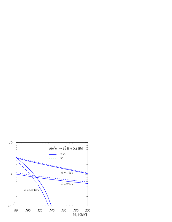
Figure 5: Cross-sections for $e^{+}e^{-}\to t\overline{t}h_{\rm SM}$ in fb for three choices of center-of-mass energy. The dashed lines correspond to the tree-level result [23], and the solid lines include the next-to-leading order QCD corrections [24].

Other relevant processes for producing Higgs bosons are associated production with a fermion-antifermion pair, and multi-Higgs production. For the former class, only $e^{+}e^{-}\to t\overline{t}h_{\rm SM}$ has a significant cross section, around the femtobarn level in the Standard Model, as depicted in Fig. 5. As a result, if $m_{h_{\rm SM}}$ is small enough (or $\sqrt{s}$ is large enough), this process can be used for determining the Higgs–top quark Yukawa coupling. The cross section for double Higgs production ($e^{+}e^{-}\to Zh_{\rm SM}h_{\rm SM}$) are even smaller, of order 0.1 fb for $100~{}{\rm GeV}\mathrel{\raise 1.29167pt\hbox{$<$\kern-7.5pt\lower 4.30554pt\hbox{$\sim$}}}m_{h_{\rm SM}}\mathrel{\raise 1.29167pt\hbox{$<$\kern-7.5pt\lower 4.30554pt\hbox{$\sim$}}}150$ GeV and $\sqrt{s}$ ranging between 500 GeV and 1 TeV. With sufficient luminosity, the latter can be used for extracting the triple Higgs self-coupling.

At the $\gamma\gamma$ collider, a Higgs boson is produced as an $s$-channel resonance via the one-loop triangle diagram. Every charged particle whose mass is generated by the Higgs boson contributes to this process. In the Standard Model, the main contributors are the $W^{\pm}$ and the $t$-quark loops. See Section 10 for further discussion.

4 SM Higgs searches before the linear collider

1 Direct search limits from LEP

The LEP collider completed its final run in 2000, and presented tantalizing hints for the possible observation of the Higgs boson. Combining data from all four LEP collaborations [10], one could interpret their observations as corresponding to the production of a Higgs boson with a mass of $m_{h^{0}}=115.0^{+1.3}_{-0.9}$ GeV with a significance of $2.9\sigma$. This is clearly not sufficient to announce a discovery or even an “observation”. A more conservative interpretation of the data then places a 95% CL lower limit of $m_{h_{\rm SM}}>113.5$ GeV.

2 Implications of precision electroweak measurements

Indirect constraints on the Higgs boson mass within the SM can be obtained from confronting the SM predictions with results of electroweak precision measurements. In the case of the top quark mass, the indirect determination turned out to be in remarkable agreement with the actual experimental value. In comparison, to obtain constraints on $m_{h_{\rm SM}}$ of similar precision, much higher accuracy is required for both the experimental results and the theory predictions. This is due to the fact that the leading dependence of the precision observables on $m_{h_{\rm SM}}$ is only logarithmic, while the dominant effects of the top-quark mass enter quadratically.

Figure 6: The prediction for $m_{W}$ as a function of $m_{h_{\rm SM}}$ is compared with the experimental value of $m_{W}$ for the current experimental accuracies of $m_{W}$ and $m_{t}$ (left plot) and for the prospective future accuracies at a LC with Giga-Z option (right plot, the present experimental central values are assumed) [25]. In the left plot also the present experimental 95% CL lower bound on the Higgs-boson mass, $m_{h_{\rm SM}}=113.5$ GeV, is indicated.

The left plot of Fig. 6 shows the currently most precise result for $m_{W}$ as function of $m_{h_{\rm SM}}$ in the SM, and compares it with the present experimental value of $m_{W}$. The calculation incorporates the complete electroweak fermion-loop contributions at ${\cal O}(\alpha^{2})$ [25]. Based on this result, the remaining theoretical uncertainty from unknown higher-order corrections has been estimated to be about $6~{}\mbox{MeV}$ [25]. It is about a factor five smaller than the uncertainty induced by the current experimental error on the top-quark mass, $\Delta m_{t}^{\rm exp}=\pm 5.1{\rm\,GeV}$, which presently dominates the theoretical uncertainty. The right plot of Fig. 6 shows the prospective situation at a future $e^{+}e^{-}$ linear collider after Giga-Z operation and a threshold measurement of the $W$ mass (keeping the present experimental central values for simplicity), which are expected to reduce the experimental errors to $\Delta m_{W}^{\rm exp}=6~{}\mbox{MeV}$ and $\Delta m_{t}^{\rm exp}=200~{}\mbox{MeV}$. This program is described in Chapter 8. The plot clearly shows the considerable improvement in the sensitivity to $m_{h_{\rm SM}}$ achievable at the LC via very precise measurements of $m_{W}$ and $m_{t}$. Since furthermore the experimental error of $\sin^{2}\theta_{w}^{\mathrm{eff}}$ is expected to be reduced by almost a factor of 20 at Giga-Z, the accuracy in the indirect determination of the Higgs-boson mass from all data will improve by about a factor of 10 compared to the present situation [26].

3 Expectations for Tevatron searches

The upgraded Tevatron began taking data in the spring of 2001. This is the only collider at which the Higgs boson can be produced for the next five years, until the LHC begins operation in 2006. The Tevatron Higgs working group presented a detailed analysis of the Higgs discovery reach at the upgraded Tevatron [27]. Here, we summarize the main results. Two Higgs mass ranges were considered separately: (i) 100 GeV$\mathrel{\raise 1.29167pt\hbox{$<$\kern-7.5pt\lower 4.30554pt\hbox{$\sim$}}}m_{h_{\rm SM}}\mathrel{\raise 1.29167pt\hbox{$<$\kern-7.5pt\lower 4.30554pt\hbox{$\sim$}}}135$ GeV and (ii) 135 GeV$\mathrel{\raise 1.29167pt\hbox{$<$\kern-7.5pt\lower 4.30554pt\hbox{$\sim$}}}m_{h_{\rm SM}}\mathrel{\raise 1.29167pt\hbox{$<$\kern-7.5pt\lower 4.30554pt\hbox{$\sim$}}}190$ GeV, corresponding to the two different dominant Higgs decay modes: $h_{\rm SM}\to b\overline{b}$ for the lighter mass range and $h_{\rm SM}\to WW^{(*)}$ for the heavier mass range.

In mass range (i), the relevant production mechanisms are $q_{i}\overline{q}_{j}\to Vh_{\rm SM}$, where $V=W$ or $Z$. In all cases, the dominant $h_{\rm SM}\to b\overline{b}$ decay was employed. The most relevant final-state signatures correspond to events in which the vector boson decays leptonically ($W\to\ell\nu$, $Z\to\ell^{+}\ell^{-}$ and $Z\to\nu\overline{\nu}$, where $\ell=e$ or $\mu$), resulting in $\ell\nu b\overline{b}$, $\nu\overline{\nu}b\overline{b}$ and $\ell^{+}\ell^{-}b\overline{b}$ final states. In mass range (ii), the relevant production mechanisms include $gg\to h_{\rm SM}$, $V^{*}V^{*}\to h_{\rm SM}$ and $q_{i}\overline{q}_{j}\to Vh_{\rm SM}$, with decays $h_{\rm SM}\to WW^{(*)}$, $ZZ^{(*)}$. The most relevant phenomenological signals are those in which two of the final-state vector bosons decay leptonically, resulting in $\ell^{+}\ell^{-}\nu\overline{\nu}$ or $\ell^{\pm}\ell^{\pm}jjX$, where $j$ is a hadronic jet and $X$ consists of two additional leptons (either charged or neutral). For example, the latter can arise from $Wh_{\rm SM}$ production followed by $h_{\rm SM}\to WW^{(*)}$, where the two like-sign $W$ bosons decay leptonically, and the third $W$ decays into hadronic jets. In this case $X$ is a pair of neutrinos.

Figure 7: The integrated luminosity required per experiment, to either exclude a SM Higgs boson at 95% CL or discover it at the $3\sigma$ or $5\sigma$ level, as a function of the Higgs mass. These results are based on the combined statistical power of both experiments. The curves shown are obtained by combining the $\ell\nu b\overline{b}$, $\nu\overline{\nu}b\overline{b}$ and $\ell^{+}\ell^{-}b\overline{b}$ channels using the neural network selection in the low-mass Higgs region ($90~{}{\rm GeV}~{}\mathrel{\raise 1.29167pt\hbox{$<$\kern-7.5pt\lower 4.30554pt\hbox{$\sim$}}}m_{h_{\rm SM}}\mathrel{\raise 1.29167pt\hbox{$<$\kern-7.5pt\lower 4.30554pt\hbox{$\sim$}}}130$ GeV), and the $\ell^{\pm}\ell^{\pm}jjX$ and $\ell^{+}\ell^{-}\nu\overline{\nu}$ channels in the high-mass Higgs region ($130~{}{\rm GeV}~{}\mathrel{\raise 1.29167pt\hbox{$<$\kern-7.5pt\lower 4.30554pt\hbox{$\sim$}}}m_{h_{\rm SM}}\mathrel{\raise 1.29167pt\hbox{$<$\kern-7.5pt\lower 4.30554pt\hbox{$\sim$}}}190$ GeV). The lower edge of the bands is the calculated threshold; the bands extend upward from these nominal thresholds by 30% as an indication of the uncertainties in $b$-tagging efficiency, background rate, mass resolution, and other effects.

Figure 7 summarizes the Higgs discovery reach versus the total integrated luminosity delivered to the Tevatron (and by assumption, delivered to each detector). As the plot shows, the required integrated luminosity increases rapidly with Higgs mass to 140 GeV, beyond which the high-mass channels play the dominant role. With 2 fb^-1 per detector (which is expected after one year of running at design luminosity), the 95% CL limits will barely extend the expected LEP2 limits, but with 10 fb^-1, the SM Higgs boson can be excluded up to 180 GeV if the Higgs boson does not exist in that mass range.

Current projections envision that the Tevatron, with further machine improvements, will provide an integrated luminosity of 15 fb^-1 after six years of running. If $m_{h_{\rm SM}}\simeq 115$ GeV, as suggested by LEP data, then the Tevatron experiments will be able to achieve a $5\sigma$ discovery of the Higgs boson. If no Higgs events are detected, the LEP limits will be significantly extended, with a 95% CL exclusion possible up to about $m_{h_{\rm SM}}\simeq 185$ GeV. Moreover, evidence for a Higgs boson at the $3\sigma$ level could be achieved up to about $m_{h_{\rm SM}}\simeq 175$ GeV. (The Higgs mass region around 140 GeV might require more luminosity, depending on the magnitude of systematic errors due to uncertainties in $b$-tagging efficiency, background rate, the $b\overline{b}$ mass resolution, etc.) Evidence for or discovery of a Higgs boson at the Tevatron would be a landmark in high energy physics. However, even if a Higgs boson is seen, the Tevatron data would only provide a very rough phenomenological profile. In contrast, the LC, and to a lesser extent, the LHC could measure enough of its properties with sufficient precision to verify that the observed Higgs is truly SM-like. The LHC is also certain to yield $>5\sigma$ discovery of a SM Higgs boson over the full range of possible masses, up to 1 TeV.

4 Expectations for LHC searches

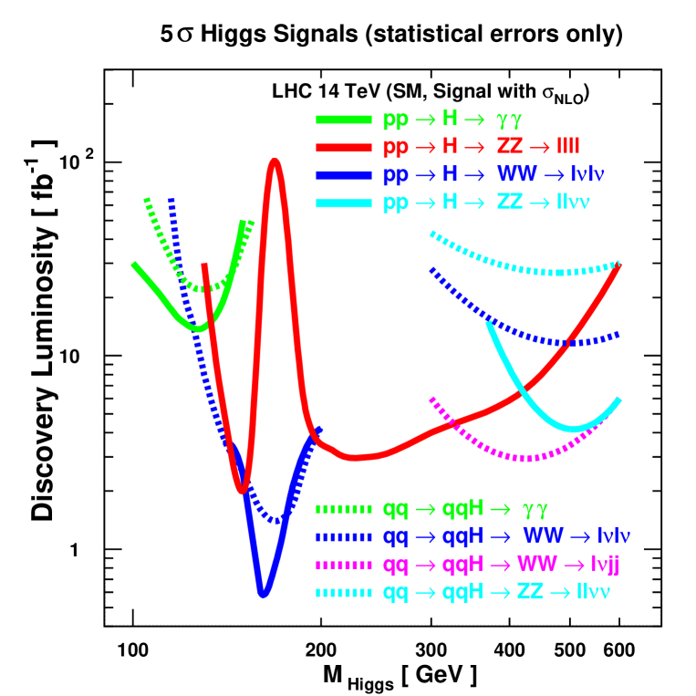
Figure 8: Expected $5\sigma$ SM Higgs discovery luminosity requirements at the LHC, for one experiment, statistical errors only [28]. The study was performed with CMS fast detector simulation.

At the LHC, the ATLAS and CMS detectors have been specifically designed so as to guarantee discovery of a SM Higgs boson, regardless of mass. The most important production processes for the $h_{\rm SM}$ are the gluon fusion process, $gg\to h_{\rm SM}$, and the vector boson fusion process, $WW\to h_{\rm SM}$. In particular, for $m_{h_{\rm SM}}\mathrel{\raise 1.29167pt\hbox{$<$\kern-7.5pt\lower 4.30554pt\hbox{$\sim$}}}130{\rm\,GeV}$ the important discovery modes are $gg,WW\to h_{\rm SM}\to\gamma\gamma$, $\tau^{+}\tau^{-}$. At high luminosity, $q_{i}\overline{q}_{j}\to W^{\pm}h_{\rm SM}$ and $gg\to t\overline{t}h_{\rm SM}$ with $h_{\rm SM}\to\gamma\gamma$ and $h_{\rm SM}\to b\overline{b}$ should also be visible. Once $m_{h_{\rm SM}}>130{\rm\,GeV}$, $gg\to h_{\rm SM}\to ZZ^{(*)}\to 4\ell$ is extremely robust except for the small mass region with $m_{h_{\rm SM}}$ just above $2m_{W}$ in which $h_{\rm SM}\to WW$ is allowed and $B(h_{\rm SM}\to ZZ^{*})$ drops sharply. In this region, $gg,WW\to h_{\rm SM}\to WW\to\ell\nu\ell\nu$ provides a strong Higgs signal. Once $m_{h_{\rm SM}}>300{\rm\,GeV}$ ($400{\rm\,GeV}$), the final states $h_{\rm SM}\to WW\to\ell\nu jj$ and $h_{\rm SM}\to ZZ\to\ell\ell\nu\nu$, where the $h_{\rm SM}$ is produced by a combination of $gg$ and $WW$ fusion, provide excellent discovery channels. These latter allow discovery even for $m_{h_{\rm SM}}\mathrel{\raise 1.29167pt\hbox{$>$\kern-7.5pt\lower 4.30554pt\hbox{$\sim$}}}1{\rm\,TeV}$, i.e., well beyond the $m_{h_{\rm SM}}\sim 800{\rm\,GeV}$ limit of viability for the $h_{\rm SM}\to 4\ell$ mode. These results are summarized in Fig. 8, from which we observe that the net statistical significance for the $h_{\rm SM}$, after combining channels, exceeds $10\sigma$ for all $m_{h_{\rm SM}}>80{\rm\,GeV}$, assuming accumulated luminosity of $L=100~{}\mbox{fb${}^{-1}$}$ at the ATLAS detector [29]. Similar results are obtained by the CMS group [30], the $\gamma\gamma$ mode being even stronger in the lower mass region.

Figure 9: Relative accuracy expected at the LHC with 200 fb^-1 of data. (a) Cross section times branching fraction for several inclusive modes (dotted and dash-dotted lines) and vector boson fusion channels (dashed and solid lines). (b) Extracted total width (solid line) and $H\to WW$ partial width (dashed line). In the latter, $\epsilon=1-[B(H\to b\overline{b})+B(H\to\tau\tau)+B(H\to WW^{(*)})+B(H\to ZZ^{(*)})+B(H\to gg)+B(H\to\gamma\gamma)]$. To the extent that $\epsilon$ is small, the indicated accuracies can be achieved.

Precision measurements for a certain number of quantities will be possible, depending upon the exact value of $m_{h_{\rm SM}}$. For instance, in [29] it is estimated that $m_{h_{\rm SM}}$ can be measured to $<0.1\%$ for $m_{h_{\rm SM}}<400{\rm\,GeV}$ and to $0.1$–$1\%$ for $400<m_{h_{\rm SM}}<700{\rm\,GeV}$. Using the $4\ell$ final state, $\Gamma^{T}_{h_{\rm SM}}$ can determined for $m_{h_{\rm SM}}>250{\rm\,GeV}$ from the shape of the $4\ell$ mass peak. Various ratios of branching ratios and a selection of partial widths times branching ratios can be measured in any given mass region. Some early estimates of possibilities and achievable accuracies appear in [2]. A more recent, but probably rather optimistic parton-level theoretical study [31] finds that if $m_{h_{\rm SM}}\mathrel{\raise 1.29167pt\hbox{$<$\kern-7.5pt\lower 4.30554pt\hbox{$\sim$}}}200{\rm\,GeV}$ then good accuracies can be achieved for many absolute partial widths and for the total width provided: (a) $WW$ fusion production can be reliably separated from $gg$ fusion; (b) the $WW/ZZ$ coupling ratio is as expected in the SM from the SU(2)$\times$U(1) symmetry; (c) the $WW^{*}$ final state can be observed in both $gg$ and $WW$ fusion; and (d) there are no unexpected decays of the $h_{\rm SM}$. Invisible Higgs decays may also be addressed by this technique [32]; CMS simulations show some promise for this channel. The resulting errors estimated for $L=200~{}\mbox{fb${}^{-1}$}$ of accumulated data are given in Fig. 9.

5 Higgs bosons in low-energy supersymmetry

The simplest realistic model of low-energy supersymmetry is the minimal supersymmetric Standard Model (MSSM), which consists of the two-Higgs-doublet extension of the Standard Model plus the corresponding superpartners [21]. Two Higgs doublets, one with $Y=+1$ and one with $Y=-1$, are needed in order that gauge anomalies due to the higgsino superpartners are exactly canceled. The supersymmetric structure also constrains the Higgs-fermion interactions. In particular, it is the $Y=-1$ Higgs doublet that generates mass for “up”-type quarks and the $Y=+1$ Higgs doublet that generates mass for “down”-type quarks (and charged leptons) [33, 34].

After electroweak symmetry breaking, one finds five physical Higgs particles: a charged Higgs pair ($H^{\pm}$), two CP-even neutral Higgs bosons (denoted by $h^{0}$ and $H^{0}$ where $m_{h^{0}}\leq m_{H^{0}}$) and one CP-odd neutral Higgs boson ($A^{0}$). Two other relevant parameters are the ratio of neutral Higgs vacuum expectation values, $\tan\beta$, and an angle $\alpha$ that measures the component of the original $Y=\pm 1$ Higgs doublet states in the physical CP-even neutral scalars.

1 MSSM Higgs sector at tree-level

The supersymmetric structure of the theory imposes constraints on the Higgs sector of the model [35]. As a result, all Higgs sector parameters at tree-level are determined by two free parameters: $\tan\beta$ and one Higgs mass, conveniently chosen to be $m_{A^{0}}$. There is an upper bound to the tree-level mass of the light CP-even Higgs boson: $m_{h^{0}}^{2}\leq m_{Z}^{2}\cos 2\beta\leq m_{Z}^{2}$. However, radiative corrections can significantly alter this upper bound as described in Section 2.

The limit of $m_{A^{0}}\gg m_{Z}$ is of particular interest, with two key consequences. First, $m_{A^{0}}\simeq m_{H^{0}}\simeq m_{H^{\pm}}$, up to corrections of ${\cal O}(m_{Z}^{2}/m_{A^{0}})$. Second, $\cos(\beta-\alpha)=0$ up to corrections of ${\cal O}(m_{Z}^{2}/m_{A^{0}}^{2})$. This limit is known as the decoupling limit [36] because when $m_{A^{0}}$ is large, the effective low-energy theory below the scale of $m_{A^{0}}$ contains a single CP-even Higgs boson, $h^{0}$, whose properties are nearly identical to those of the Standard Model Higgs boson, $h_{\rm SM}$.

The phenomenology of the Higgs sector is determined by the various couplings of the Higgs bosons to gauge bosons, Higgs bosons and fermions. The couplings of the two CP-even Higgs bosons to $W$ and $Z$ pairs are given in terms of the angles $\alpha$ and $\beta$ by

$$g_{h^{0}VV} = g_{V}m_{V}\sin(\beta-\alpha)$$

$$g_{H^{0}VV} = g_{V}m_{V}\cos(\beta-\alpha)\,,$$ (3)

where

$$g_{V}\equiv\begin{array}[]{cl}g,&V=W,\\ g/\cos\theta_{W},&V=Z.\end{array}$$ (4)

There are no tree-level couplings of $A^{0}$ or $H^{\pm}$ to $VV$. The couplings of one gauge boson to two neutral Higgs bosons are given by:

$$g_{h^{0}A^{0}Z} = {g\cos(\beta-\alpha)\over 2\cos\theta_{W}}\,,$$

$$g_{H^{0}A^{0}Z} = {-g\sin(\beta-\alpha)\over 2\cos\theta_{W}}\,.$$ (5)

In the MSSM, the Higgs tree-level couplings to fermions obey the following property: the neutral member of the $Y=-1$ [$Y=+1$] Higgs doublet couples exclusively to down-type [up-type] fermion pairs. This pattern of Higgs-fermion couplings defines the Type-II two-Higgs-doublet model [37, 1]. Consequently, the couplings of the neutral Higgs bosons to $f\overline{f}$ relative to the Standard Model value, $gm_{f}/2m_{W}$, are given by (using third family notation):

$$h^{0}b\overline{b}\;\;\;({\rm or}~{}h^{0}\tau^{+}\tau^{-}) : ~{}~{}-{\sin\alpha\over\cos\beta}=\sin(\beta-\alpha)-\tan\beta\cos(\beta-\alpha)\,,$$

$$h^{0}t\overline{t} : ~{}~{}\phantom{-}{\cos\alpha\over\sin\beta}=\sin(\beta-\alpha)+\cot\beta\cos(\beta-\alpha)\,,$$

$$H^{0}b\overline{b}\;\;\;({\rm or}~{}H^{0}\tau^{+}\tau^{-}) : ~{}~{}\phantom{-}{\cos\alpha\over\cos\beta}=\cos(\beta-\alpha)+\tan\beta\sin(\beta-\alpha)\,,$$

$$H^{0}t\overline{t} : ~{}~{}\phantom{-}{\sin\alpha\over\sin\beta}=\cos(\beta-\alpha)-\cot\beta\sin(\beta-\alpha)\,,$$

$$A^{0}b\overline{b}\;\;\;({\rm or}~{}A^{0}\tau^{+}\tau^{-}) : ~{}~{}\phantom{-}\gamma_{5}\,{\tan\beta}\,,$$

$$A^{0}t\overline{t} : ~{}~{}\phantom{-}\gamma_{5}\,{\cot\beta}\,.$$ (6)

In these expressions, $\gamma_{5}$ indicates a pseudoscalar coupling.

The neutral Higgs boson couplings to fermion pairs (1) have been written in such a way that their behavior can be immediately ascertained in the decoupling limit ($m_{A^{0}}\gg m_{Z}$) by setting $\cos(\beta-\alpha)=0$. In particular, in the decoupling limit, the couplings of $h^{0}$ to vector bosons and fermion pairs are equal to the corresponding couplings of the Standard Model Higgs boson.

The region of MSSM Higgs sector parameter space in which the decoupling limit applies is large, because $\sin(\beta-\alpha)$ approaches 1 quite rapidly once $m_{A^{0}}$ is larger than about 200 GeV, as shown in Fig. 10. As a result, over a significant region of the MSSM parameter space, the search for the lightest CP-even Higgs boson of the MSSM is equivalent to the search for the Standard Model Higgs boson. This result is more general; in many theories of non-minimal Higgs sectors, there is a significant portion of the parameter space that approximates the decoupling limit. Consequently, simulations of the Standard Model Higgs signal are also relevant for exploring the more general Higgs sector.

Figure 10: The value of $\sin^{2}(\beta-\alpha)$ is shown as a function of $m_{A^{0}}$ for two choices of $\tan\beta=3$ and $\tan\beta=30$. When radiative corrections are included, one can define an approximate loop-corrected angle $\alpha$ as a function of $m_{A^{0}}$, $\tan\beta$ and the MSSM parameters. In the figures above, we have incorporated radiative corrections, assuming that $M_{\rm SUSY}=1$ TeV. In addition, two extreme cases for the squark mixing parameters are shown (see Section 2 for further discussion of the radiative corrections and their dependence on the supersymmetric parameters). The decoupling effect expected when $\sin^{2}(\beta-\alpha)\simeq 1$ for $m_{A^{0}}\gg m_{Z}$, continues to hold even when radiative corrections are included.

2 The radiatively corrected MSSM Higgs sector

When one-loop radiative corrections are incorporated, the Higgs masses and couplings depend on additional parameters of the supersymmetric model that enter via the virtual loops. One of the most striking effects of the radiative corrections to the MSSM Higgs sector is the modification of the upper bound of the light CP-even Higgs mass, as first noted in [38]. When $\tan\beta\gg 1$ and $m_{A^{0}}\gg m_{Z}$, the tree-level prediction for $m_{h^{0}}$ corresponds to its theoretical upper bound, $m_{h}^{\rm max}=m_{Z}$. Including radiative corrections, the theoretical upper bound is increased, primarily because of an incomplete cancellation of the top-quark and top-squark (stop) loops. (These contributions would cancel if supersymmetry were exact.) The relevant parameters that govern the stop sector are the average of the two stop squared-masses: $M^{2}_{\rm SUSY}\equiv\frac{1}{2}(M_{\widetilde{t}_{1}}^{2}+M_{\widetilde{t}_{2}}^{2})$, and the off-diagonal element of the stop squared-mass matrix: $m_{t}X_{t}\equiv m_{t}(A_{t}-\mu\cot\beta)$, where $A_{t}$ is a soft supersymmetry-breaking trilinear scalar interaction term, and $\mu$ is the supersymmetric Higgs mass parameter. The qualitative behavior of the radiative corrections can be most easily seen in the large top squark mass limit, where, in addition, the splitting of the two diagonal entries and the off-diagonal entry of the stop squared-mass matrix are both small in comparison to $M^{2}_{\rm SUSY}$. In this case, the upper bound on the lightest CP-even Higgs mass is approximately given by

$$m_{h^{0}}^{2}\mathrel{\raise 1.29167pt\hbox{$<$\kern-7.5pt\lower 4.30554pt\hbox{$\sim$}}}m_{Z}^{2}+{3g^{2}m_{t}^{4}\over 8\pi^{2}m_{W}^{2}}\left[\ln\left({M^{2}_{\rm SUSY}\over m_{t}^{2}}\right)+{X_{t}^{2}\over M^{2}_{\rm SUSY}}\left(1-{X_{t}^{2}\over 12M^{2}_{\rm SUSY}}\right)\right]\,.$$ (7)

More complete treatments of the radiative corrections include the effects of stop mixing, renormalization group improvement, and the leading two-loop contributions, and imply that these corrections somewhat overestimate the true upper bound of $m_{h^{0}}$ (see [39] for the most recent results). Nevertheless, Eq. (7) correctly illustrates some noteworthy features of the more precise result. First, the increase of the light CP-even Higgs mass bound beyond $m_{Z}$ can be significant. This is a consequence of the $m_{t}^{4}$ enhancement of the one-loop radiative correction. Second, the dependence of the light Higgs mass on the stop mixing parameter $X_{t}$ implies that (for a given value of $M_{\rm SUSY}$) the upper bound of the light Higgs mass initially increases with $X_{t}$ and reaches its maximal value at $X_{t}\simeq\sqrt{6}M_{\rm SUSY}$. This point is referred to as the maximal mixing case (whereas $X_{t}=0$ corresponds to the minimal mixing case).

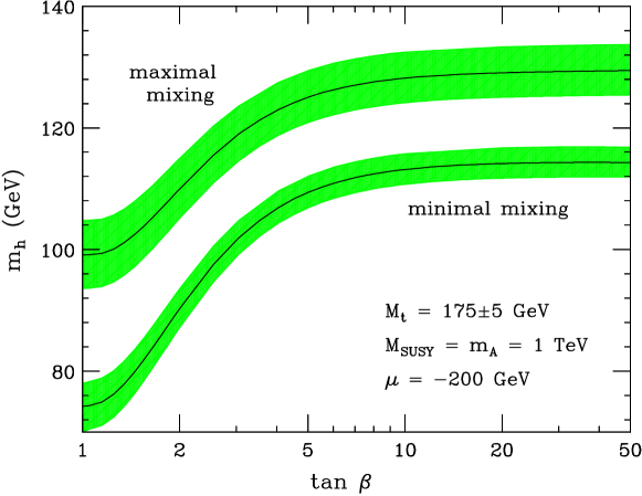
Figure 11: The radiatively corrected light CP-even Higgs mass is plotted as a function of $\tan\beta$, for the maximal mixing [upper band] and minimal mixing cases. The impact of the top quark mass is exhibited by the shaded bands; the central value corresponds to $m_{t}=175$ GeV, while the upper [lower] edge of the bands correspond to increasing [decreasing] $m_{t}$ by 5 GeV.

Taking $m_{A^{0}}$ large, Fig. 11 illustrates that the maximal value of the lightest CP-even Higgs mass bound is realized at large $\tan\beta$ in the case of maximal mixing. Allowing for the uncertainty in the measured value of $m_{t}$ and the uncertainty inherent in the theoretical analysis, one finds for $M_{\rm SUSY}\mathrel{\raise 1.29167pt\hbox{$<$\kern-7.5pt\lower 4.30554pt\hbox{$\sim$}}}2$ TeV that $m_{h^{0}}\mathrel{\raise 1.29167pt\hbox{$<$\kern-7.5pt\lower 4.30554pt\hbox{$\sim$}}}m_{h}^{\rm max}$, where

$$m_{h}^{\rm max} \simeq 122~{}{\rm GeV},\quad\mbox{minimal stop mixing,}$$

$$m_{h}^{\rm max} \simeq 135~{}{\rm GeV},\quad\mbox{maximal stop mixing.}$$ (8)

The $h^{0}$ mass bound in the MSSM quoted above does not apply to non-minimal supersymmetric extensions of the Standard Model. If additional Higgs singlet and/or triplet fields are introduced, then new Higgs self-coupling parameters appear, which are not significantly constrained by present data. For example, in the simplest non-minimal supersymmetric extension of the Standard Model (NMSSM), the addition of a complex Higgs singlet field $S$ adds a new Higgs self-coupling parameter, $\lambda_{S}$ [40]. The mass of the lightest neutral Higgs boson can be raised arbitrarily by increasing the value of $\lambda_{S}$, analogous to the behavior of the Higgs mass in the Standard Model. Under the assumption that all couplings stay perturbative up to the Planck scale, one finds in essentially all cases that $m_{h^{0}}\mathrel{\raise 1.29167pt\hbox{$<$\kern-7.5pt\lower 4.30554pt\hbox{$\sim$}}}200$ GeV, independent of the details of the low-energy supersymmetric model [41].

Figure 12: Lightest CP-even Higgs mass ($m_{h^{0}}$), heaviest CP-even Higgs mass ($m_{H^{0}}$) and charged Higgs mass ($m_{H^{\pm}}$) as a function of $m_{A^{0}}$ for two choices of $\tan\beta=3$ and $\tan\beta=30$. The slight increase in the charged Higgs mass as $\tan\beta$ is increased from 3 to 30 is a consequence of the radiative corrections.

In Fig. 12, we exhibit the masses of the CP-even neutral and the charged Higgs masses as a function of $m_{A^{0}}$. Note that $m_{H^{0}}\geq m_{h}^{\rm max}$ for all values of $m_{A^{0}}$ and $\tan\beta$, where $m_{h}^{\rm max}$ is to be evaluated depending on the top-squark mixing, as indicated in Eq. (2).

Radiative corrections also significantly modify the tree-level values of the Higgs boson couplings to fermion pairs and to vector boson pairs. As discussed above, the tree-level Higgs couplings depend crucially on the value of $\sin(\beta-\alpha)$. In the first approximation, when radiative corrections of the Higgs squared-mass matrix are computed, the diagonalizing angle $\alpha$ is modified. This provides one important source of the radiative corrections of the Higgs couplings. In Fig. 10, we show the effect of radiative corrections on the value of $\sin(\beta-\alpha)$ as a function of $m_{A^{0}}$ for different values of the squark mixing parameters and $\tan\beta$. One can then simply insert the radiatively corrected value of $\alpha$ into eqs. (3), (5), and (1) to obtain radiatively improved couplings of Higgs bosons to vector bosons and to fermions.

At large $\tan\beta$, there is another potentially important class of radiative corrections in addition to those that enter through the modified $\alpha$. These corrections arise in the relation between $m_{b}$ and $\tan\beta$ and depend on the details of the MSSM spectrum (which enter via loop-effects). At tree-level, the Higgs couplings to $b\overline{b}$ are proportional to the Higgs–bottom-quark Yukawa coupling. Deviations from the tree-level relation due to radiative corrections are calculable and finite [42, 43, 44, 45, 46]. One of the fascinating properties of such corrections is that in certain cases the corrections do not vanish in the limit of large supersymmetric mass parameters. These corrections grow with $\tan\beta$ and therefore can be significant in the large $\tan\beta$ limit. In the supersymmetric limit, $b\overline{b}$ couples only to the neutral component of the $Y=-1$ Higgs doublet. However, when supersymmetry is broken there will be a small coupling of $b\overline{b}$ to the neutral component of the $Y=+1$ Higgs doublet resulting from radiative corrections. From this result, one can compute the couplings of the physical Higgs bosons to $b\overline{b}$ pairs. A useful approximation at large $\tan\beta$ yields the following corrections to Eq. (1):

$$h^{0}b\overline{b} : ~{}~{}~{}-{\sin\alpha\over\cos\beta}{1\over 1+\Delta_{b}}\left[1-\frac{\Delta_{b}\cot\alpha}{\tan\beta}\right]\,,$$

$$H^{0}b\overline{b} : ~{}~{}~{}\phantom{-}{\cos\alpha\over\cos\beta}{1\over 1+\Delta_{b}}\left[1+\frac{\Delta_{b}\tan\alpha}{\tan\beta}\right]\,,$$

$$A^{0}b\overline{b} : ~{}~{}~{}\phantom{-}\gamma_{5}\,\frac{\tan\beta}{1+\Delta_{b}}\,,$$ (9)

where $\Delta_{b}\propto\tan\beta$. The explicit form of $\Delta_{b}$ at one–loop in the limit of $M_{\rm SUSY}\gg m_{b}$ is given in [43, 44, 45]. The correction $\Delta_{b}$ arises from a bottom-squark–gluino loop, which depends on the gluino mass and the supersymmetric Higgs mass parameter $\mu$, and the top-squark–chargino loop, which depends on the top-squark masses and the top-squark mixing parameters $\mu$ and $A_{t}$. Contributions proportional to the electroweak gauge couplings have been neglected.

Similarly, the neutral Higgs couplings to $\tau^{+}\tau^{-}$ are modified by replacing $\Delta_{b}$ in Eq. (2) with $\Delta_{\tau}$ [44, 45]. One can also derive radiatively corrected couplings of the charged Higgs boson to fermion pairs [47, 48]. The tree-level couplings of the charged Higgs boson to fermion pairs are modified accordingly by replacing $m_{b}\rightarrow m_{b}/(1+\Delta_{b})$ and $m_{\tau}\rightarrow m_{\tau}/(1+\Delta_{\tau})$, respectively.

One consequence of the above results is that the neutral Higgs coupling to $b\overline{b}$ (which is expected to be the dominant decay mode over nearly all of the MSSM Higgs parameter space), can be significantly suppressed at large $\tan\beta$ [49, 50, 51] if $\Delta_{b}\simeq{\cal O}(1)$. Typically $|\Delta_{\tau}|\ll|\Delta_{b}|$, since the correction proportional to $\alpha_{s}$ in the latter is absent in the former. For this reason, the $\tau^{+}\tau^{-}$ decay mode can be the dominant Higgs decay channel for the CP-even Higgs boson with SM-like couplings to gauge bosons.

In the decoupling limit, one can show that $\cot\alpha\cot\beta=-1+{\cal O}(m_{Z}^{2}/m_{A^{0}}^{2})$. Inserting this result into Eq. (2), one can check that the $h^{0}b\overline{b}$ coupling does indeed approach its Standard Model value. However, because $\Delta_{b}\propto\tan\beta$, the deviation of the $h^{0}b\overline{b}$ coupling from the corresponding SM result is of ${\cal O}(m_{Z}^{2}\tan\beta/m_{A^{0}}^{2})$. That is, at large $\tan\beta$, the approach to decoupling may be “delayed” [52], depending on the values of other MSSM parameters that enter the radiative corrections.

3 MSSM Higgs boson decay modes

In this section, we consider the decay properties of the three neutral Higgs bosons ($h^{0}$, $H^{0}$ and $A^{0}$) and of the charged Higgs pair ($H^{\pm}$). Let us start with the lightest state, $h^{0}$. When $m_{A^{0}}\gg m_{Z}$, the decoupling limit applies, and the couplings of $h^{0}$ to SM particles are nearly indistinguishable from those of $h_{\rm SM}$. If some superpartners are light, there may be some additional decay modes, and hence the $h^{0}$ branching ratios would be different from the corresponding Standard Model values, even though the partial widths to Standard Model particles are the same. Furthermore, loops of light charged or colored superpartners could modify the $h^{0}$ coupling to photons and/or gluons, in which case the one-loop $gg$ and $\gamma\gamma$ decay rates would also be different. On the other hand, if all superpartners are heavy, all the decay properties of $h^{0}$ are essentially those of the SM Higgs boson, and the discussion of Section 1 applies.

The heavier Higgs states, $H^{0}$, $A^{0}$ and $H^{\pm}$, are roughly mass-degenerate and have negligible couplings to vector boson pairs. In particular, $\Gamma(H^{0}\to VV)\ll\Gamma(h_{\rm SM}\to VV)$, while the couplings of $A^{0}$ and $H^{\pm}$ to the gauge bosons are loop-suppressed. The couplings of $H^{0}$, $A^{0}$ and $H^{\pm}$ to down-type (up-type) fermions are significantly enhanced (suppressed) relative to those of $h_{\rm SM}$ if $\tan\beta\gg 1$. Consequently, the decay modes $H^{0},A^{0}\to b\overline{b}$, $\tau^{+}\tau^{-}$ dominate the neutral Higgs decay modes for moderate-to-large values of $\tan\beta$ below the $t\overline{t}$ threshold, while $H^{+}\to\tau^{+}\nu$ dominates the charged Higgs decay below the $t\overline{b}$ threshold.

For values of $m_{A^{0}}$ of order $m_{Z}$, all Higgs boson states lie below 200 GeV in mass, and would all be accessible at the LC. In this parameter regime, there is a significant area of the parameter space in which none of the neutral Higgs boson decay properties approximates those of $h_{\rm SM}$. For example, when $\tan\beta$ is large, supersymmetry-breaking effects can significantly modify the $b\overline{b}$ and/or the $\tau^{+}\tau^{-}$ decay rates with respect to those of $h_{\rm SM}$. Additionally, the heavier Higgs bosons can decay into lighter Higgs bosons. Examples of such decay modes are: $H^{0}\to h^{0}h^{0}$, $A^{0}A^{0}$, and $ZA^{0}$, and $H^{\pm}\to W^{\pm}h^{0}$, $W^{\pm}A^{0}$ (although in the MSSM, the Higgs branching ratio into vector boson–Higgs boson final states, if kinematically allowed, rarely exceeds a few percent). The decay of the heavier Higgs boson into two lighter Higgs bosons can provide information about Higgs self-couplings. For values of $\tan\beta\mathrel{\raise 1.29167pt\hbox{$<$\kern-7.5pt\lower 4.30554pt\hbox{$\sim$}}}5$, the branching ratio of $H^{0}\to h^{0}h^{0}$ is dominant for a Higgs mass range of $200~{}{\rm GeV}\mathrel{\raise 1.29167pt\hbox{$<$\kern-7.5pt\lower 4.30554pt\hbox{$\sim$}}}m_{H^{0}}\mathrel{\raise 1.29167pt\hbox{$<$\kern-7.5pt\lower 4.30554pt\hbox{$\sim$}}}2m_{t}$. The dominant radiative corrections to this decay arise from the corrections to the self-interaction $\lambda_{H^{0}h^{0}h^{0}}$ in the MSSM and are large [53].

The phenomenology of charged Higgs bosons is less model-dependent, and is governed by the values of $\tan\beta$ and $m_{H^{\pm}}$. Because charged Higgs couplings are proportional to fermion masses, the decays to third-generation quarks and leptons are dominant. In particular, for $m_{H^{\pm}}<m_{t}+m_{b}$ (so that the channel $H^{+}\to t\overline{b}$ is closed), $H^{+}\to\tau^{+}\nu_{\tau}$ is favored if $\tan\beta\mathrel{\raise 1.29167pt\hbox{$>$\kern-7.5pt\lower 4.30554pt\hbox{$\sim$}}}1$, while $H^{+}\to c\overline{s}$ is favored only if $\tan\beta$ is small. Indeed, ${\rm BR}(H^{+}\to\tau^{+}\nu_{\tau})\simeq 1$ if $\tan\beta\mathrel{\raise 1.29167pt\hbox{$>$\kern-7.5pt\lower 4.30554pt\hbox{$\sim$}}}5$. These results apply generally to Type-II two-Higgs doublet models. For $m_{H^{\pm}}\mathrel{\raise 1.29167pt\hbox{$>$\kern-7.5pt\lower 4.30554pt\hbox{$\sim$}}}180$ GeV, the decay $H^{+}\to t\overline{b}\to W^{+}b\overline{b}$ is the dominant decay mode.

In addition to the above decay modes, there exist new Higgs decay channels that involve supersymmetric final states. Higgs decays into charginos, neutralinos and third-generation squarks and sleptons can become important, once they are kinematically allowed [54]. For Higgs masses below 130 GeV, the range of supersymmetric parameter space in which supersymmetric decays are dominant is rather narrow when the current bounds on supersymmetric particle masses are taken into account. One interesting possibility is a significant branching ratio of $h^{0}\to\widetilde{\chi}^{0}\widetilde{\chi}^{0}$, which could arise for values of $m_{h^{0}}$ near its upper theoretical limit. Such an invisible decay mode could be detected at the LC by searching for the missing mass recoiling against the $Z$ in $e^{+}e^{-}\to h^{0}Z$.

4 MSSM Higgs boson production at the LC

For $m_{A^{0}}\mathrel{\raise 1.29167pt\hbox{$>$\kern-7.5pt\lower 4.30554pt\hbox{$\sim$}}}150$ GeV, Fig. 10 shows that the MSSM Higgs sector quickly approaches the decoupling limit, where the properties of $h^{0}$ approximately coincide with those of $h_{\rm SM}$. Thus, the Higgsstrahlung and vector-boson-fusion cross-sections for $h_{\rm SM}$ production also apply to $h^{0}$ production. In contrast, the $H^{0}VV$ and $A^{0}VV$ couplings are highly suppressed, since $|\cos(\beta-\alpha)|\ll 1$. Equation (3) illustrates this for the $H^{0}W$ coupling. Thus, these mechanisms are no longer useful for $H^{0}$ and $A^{0}$ production. The most robust production mechanism is $e^{+}e^{-}\to Z^{*}\to H^{0}A^{0}$, which is not suppressed since the $ZH^{0}A^{0}$ coupling is proportional to $\sin(\beta-\alpha)$, as indicated in Eq. (5). Radiatively corrected cross-sections for $Zh^{0}$, $ZH^{0}$, $H^{0}A^{0}$, and $h^{0}A^{0}$ have been recently obtained in [55]. The charged Higgs boson is also produced in pairs via $s$-channel photon and $Z$ exchange. However, since $m_{H^{0}}\simeq m_{A^{0}}\simeq m_{H^{\pm}}$ in the decoupling limit, $H^{0}A^{0}$ and $H^{+}H^{-}$ production are kinematically allowed only when $m_{A^{0}}\mathrel{\raise 1.29167pt\hbox{$<$\kern-7.5pt\lower 4.30554pt\hbox{$\sim$}}}\sqrt{s}/2$. In $\gamma\gamma$ collisions, one can extend the Higgs mass reach for the neutral Higgs bosons. As described in Section 10, the $s$-channel resonant production of $H^{0}$ and $A^{0}$ (due primarily to the top and bottom-quark loops in the one-loop Higgs–$\gamma\gamma$ triangle) can be detected for some choices of $m_{A^{0}}$ and $\tan\beta$ if the heavy Higgs masses are less than about 80% of the initial $\sqrt{s}$ of the primary $e^{+}e^{-}$ system. The corresponding cross sections are a few fb [56, 57].

If $m_{A^{0}}\mathrel{\raise 1.29167pt\hbox{$<$\kern-7.5pt\lower 4.30554pt\hbox{$\sim$}}}150$ GeV, deviations from the decoupling limit become more apparent, and $H^{0}$ can now be produced via Higgsstrahlung and vector boson fusion at an observable rate. In addition, the factor of $\cos(\beta-\alpha)$ in the $Zh^{0}A^{0}$ coupling no longer significantly suppresses $h^{0}A^{0}$ production. Finally, if $m_{H^{\pm}}\mathrel{\raise 1.29167pt\hbox{$<$\kern-7.5pt\lower 4.30554pt\hbox{$\sim$}}}170$ GeV, the charged Higgs boson will also be produced in $t\to H^{+}b$. In the non-decoupling regime, all non-minimal Higgs states can be directly produced and studied at the LC.

The associated production of a single Higgs boson and a fermion-antifermion pair can also be considered. Here, the new feature is the possibility of enhanced Higgs–fermion Yukawa couplings. Consider the behavior of the Higgs couplings at large $\tan\beta$, where some of the Higgs couplings to down type fermion pairs (denoted generically by $b\overline{b}$) can be significantly enhanced. Let us examine two particular large $\tan\beta$ regions of interest. In the decoupling limit (where $m_{A^{0}}\gg m_{Z}$ and $|\cos(\beta-\alpha)|\ll 1$), it follows from Eq. (1) that the $b\overline{b}H^{0}$ and $b\overline{b}A^{0}$ couplings have equal strength and are significantly enhanced by a factor of $\tan\beta$ relative to the $b\overline{b}h_{\rm SM}$ coupling, while the $b\overline{b}h^{0}$ coupling is given by the corresponding Standard Model value. If $m_{A^{0}}\mathrel{\raise 1.29167pt\hbox{$<$\kern-7.5pt\lower 4.30554pt\hbox{$\sim$}}}m_{Z}$ and $\tan\beta\gg 1$, then $|\sin(\beta-\alpha)|\ll 1$, as shown in Fig. 10, and $m_{h^{0}}\simeq m_{A^{0}}$. In this case, the $b\overline{b}h^{0}$ and $b\overline{b}A^{0}$ couplings have equal strength and are significantly enhanced (by a factor of $\tan\beta$) relative to the $b\overline{b}h_{\rm SM}$ coupling. Note that in both cases above, only two of the three neutral Higgs bosons have enhanced couplings to $b\overline{b}$. If $\phi$ is one of the two neutral Higgs bosons with enhanced $b\overline{b}\phi$ couplings, then the cross-section for $e^{+}e^{-}\to f\overline{f}\phi$ ($f=b$ or $\tau$) will be significantly enhanced relative to the corresponding Standard Model cross-section by a factor of $\tan^{2}\beta$. The phase-space suppression is not as severe as in $e^{+}e^{-}\to t\overline{t}\phi$ (see Fig. 5), so this process could extend the mass reach of the heavier neutral Higgs states at the LC given sufficient luminosity. The production of the charged Higgs boson via $e^{+}e^{-}\to t\overline{b}H^{-}$ is also enhanced by $\tan^{2}\beta$, although this process has a more significant phase-space suppression because of the final state top quark. If any of these processes can be observed, it would provide a direct measurement of the corresponding Higgs–fermion Yukawa coupling.

6 MSSM Higgs boson searches before the LC

1 Review of direct search limits

Although no direct experimental evidence for the Higgs boson yet exists, there are both experimental as well as theoretical constraints on the parameters of the MSSM Higgs sector. Experimental limits on the charged and neutral Higgs masses have been obtained at LEP. For the charged Higgs boson, $m_{H^{\pm}}>78.7$ GeV [58]. This is the most model-independent bound. It is valid for more general non-supersymmetric two-Higgs doublet models and assumes only that the $H^{+}$ decays dominantly into $\tau^{+}\nu_{\tau}$ and/or $c\overline{s}$. The LEP limits on the masses of $h^{0}$ and $A^{0}$ are obtained by searching simultaneously for $e^{+}e^{-}\to Z\to Zh^{0}$ and $e^{+}e^{-}\to Z\to h^{0}A^{0}$. Radiative corrections can be significant, as shown in Section 2, so the final limits depend on the choice of MSSM parameters that govern the radiative corrections. The third generation squark parameters are the most important of these. The LEP Higgs working group [59] quotes limits for the case of $M_{\rm SUSY}=1$ TeV in the maximal-mixing scenario, which corresponds to the choice of third generation squark parameters that yields the largest corrections to $m_{h^{0}}$. The present LEP 95% CL lower limits are $m_{A^{0}}>91.9$ GeV and $m_{h^{0}}>91.0$ GeV. The theoretical upper bound on $m_{h^{0}}$ as a function of $\tan\beta$, exhibited in Fig. 11, can then be used to exclude a region of $\tan\beta$ in which the predicted value of $m_{h^{0}}$ lies below the experimental bound. Under the same MSSM Higgs parameter assumptions stated above, the LEP Higgs search excludes the region $0.5<\tan\beta<2.4$ at 95% CL.

In discussing Higgs discovery prospects at the Tevatron and LHC, we shall quote limits based on the assumption of $M_{\rm SUSY}=1$ TeV and maximal squark mixing. This tends to be a conservative assumption; that is, other choices give sensitivity to more of the $m_{A^{0}}$ versus $\tan\beta$ plane. However, there are a number of other parameter regimes in which certain Higgs search strategies become more difficult. While these issues are of vital importance to the Tevatron and LHC Higgs searches, they are much less important at the LC.

2 MSSM Higgs searches at the Tevatron

At the Tevatron, the SM Higgs search can be reinterpreted in terms of the search for the CP-even Higgs boson of the MSSM. Since the theoretical upper bound was found to be $m_{h^{0}}\mathrel{\raise 1.29167pt\hbox{$<$\kern-7.5pt\lower 4.30554pt\hbox{$\sim$}}}135$ GeV (for $M_{\rm SUSY}<2$ TeV), only the Higgs search of the low-mass region, 100 GeV $\mathrel{\raise 1.29167pt\hbox{$<$\kern-7.5pt\lower 4.30554pt\hbox{$\sim$}}}m_{h^{0}}\mathrel{\raise 1.29167pt\hbox{$<$\kern-7.5pt\lower 4.30554pt\hbox{$\sim$}}}135$ GeV, applies. In the MSSM at large $\tan\beta$, the enhancement of the $A^{0}b\overline{b}$ coupling (and a similar enhancement of either the $h^{0}b\overline{b}$ or $H^{0}b\overline{b}$ coupling) provides a new search channel: $q\overline{q}$, $gg\to b\overline{b}\phi$, where $\phi$ is a neutral Higgs boson with enhanced couplings to $b\overline{b}$. Combining both sets of analyses, the Tevatron Higgs Working Group obtained the anticipated 95% CL exclusion and 5$\sigma$ Higgs discovery contours for the maximal mixing scenario as a function of total integrated luminosity per detector (combining both CDF and D0 data sets) shown in Fig. 13 [27].

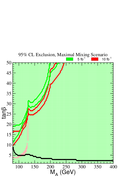
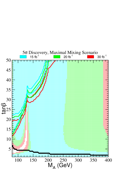
Figure 13: (a) 95$\%$ CL exclusion region and (b) $5\sigma$ discovery region on the $m_{A^{0}}$–$\tan\beta$ plane, for the maximal mixing scenario and two different search channels: $q\overline{q}\to V\phi$ ($\phi=h^{0}$, $H^{0}$), $\phi\to b\overline{b}$ (shaded regions) and $gg$, $q\overline{q}\to b\overline{b}\phi$ ($\phi=h^{0}$, $H^{0}$, $A^{0}$), $\phi\to b\overline{b}$ (region in the upper left-hand corner bounded by the solid lines). Different integrated luminosities are explicitly shown by the color coding. The two sets of lines (for a given color) correspond to the CDF and DØ simulations, respectively. The region below the solid black line near the bottom of the plot is excluded by the absence of observed $e^{+}e^{-}\to Z\phi$ events at LEP2.

From these results, one sees that 5 fb^-1 of integrated luminosity per experiment will allow one to test nearly all of the MSSM Higgs parameter space at 95% CL. To assure discovery of a CP-even Higgs boson at the 5$\sigma$ level, the luminosity requirement becomes very important. Figure 13(b) shows that a total integrated luminosity of about 20 fb^-1 per experiment is necessary in order to assure a significant, although not exhaustive, coverage of the MSSM parameter space. If the anticipated 15 fb^-1 integrated luminosity is achieved, the discovery reach will significantly extend beyond that of LEP. A Higgs discovery would be assured if the Higgs interpretation of the Higgs-like LEP events is correct. Nevertheless, the MSSM Higgs boson could still evade capture at the Tevatron. We would then turn to the LHC to try to obtain a definitive Higgs boson discovery.

3 MSSM Higgs searches at the LHC

The potential of the LHC to discover one or more of the MSSM Higgs bosons has been exhaustively studied for the minimal and maximal mixing scenarios described above. One of the primary goals of these studies has been to demonstrate that at least one of the MSSM Higgs bosons will be observed by ATLAS and CMS for any possible choice of $\tan\beta$ and $m_{A^{0}}$ consistent with bounds coming from current LEP data. In order to establish such a ‘no-lose’ theorem, an important issue is whether or not the Higgs bosons have substantial decays to supersymmetric particle pairs. It is reasonable to suppose that these decays will be absent or relatively insignificant for the light $h^{0}$. Current mass limits on SUSY particles are such that only $h^{0}\to\widetilde{\chi}^{0}_{1}\widetilde{\chi}^{0}_{1}$ might possibly be kinematically allowed and this possibility arises only in a very limited class of models. For $m_{A^{0}}\mathrel{\raise 1.29167pt\hbox{$>$\kern-7.5pt\lower 4.30554pt\hbox{$\sim$}}}200{\rm\,GeV}$, decays of the $A^{0},H^{0},H^{\pm}$ to SUSY pair states (especially pairs of light charginos/neutralinos) are certainly a possibility, but the branching ratios are generally not all that large. The discovery limits we discuss below would be weakened, but not dramatically. Further, at high $\tan\beta$ the enhancement of the $b\overline{b}$ and $\tau^{+}\tau^{-}$ couplings of the heavy $A^{0}$ and $H^{0}$ imply that SUSY decay modes will not be important even for quite high $m_{A^{0}}\sim m_{H^{0}}\sim m_{H^{\pm}}$. We will summarize the LHC discovery prospects for the MSSM Higgs bosons assuming that SUSY decays are not significant.

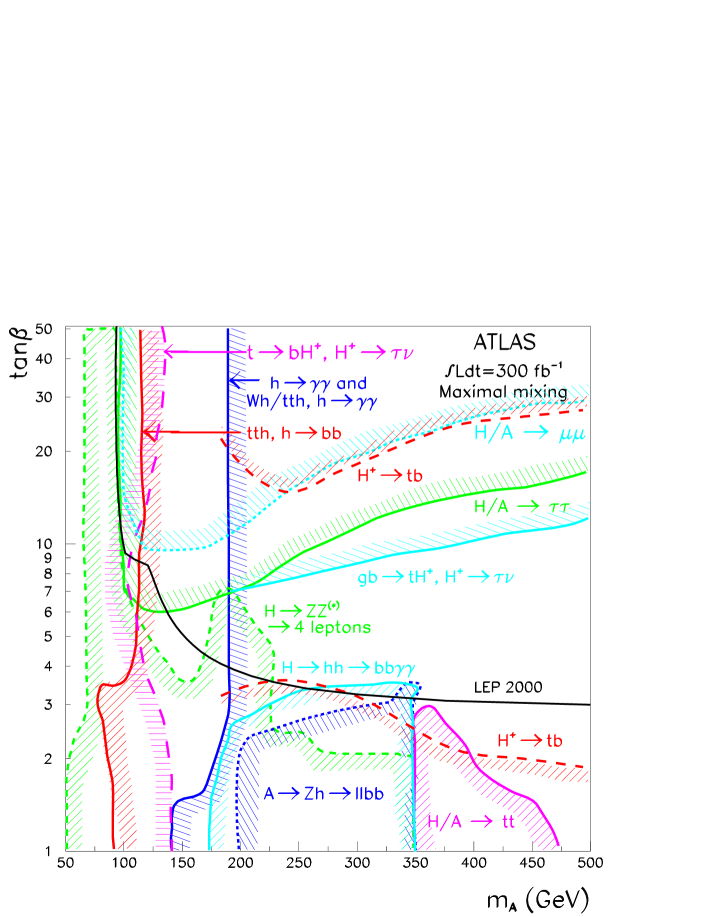
Figure 14: $5\sigma$ discovery contours for MSSM Higgs boson detection in various channels are shown in the $[m_{A^{0}},\tan\beta]$ parameter space, assuming maximal mixing and an integrated luminosity of $L=300~{}\mbox{fb${}^{-1}$}$ for the ATLAS detector. This figure is preliminary [60].

One of the primary Higgs discovery modes is detection of the relatively SM-like $h^{0}$ using the same modes as employed for a light $h_{\rm SM}$. Based on Fig. 14 (which assumes $L=300~{}\mbox{fb${}^{-1}$}$) [60], we see that for $m_{A^{0}}\mathrel{\raise 1.29167pt\hbox{$>$\kern-7.5pt\lower 4.30554pt\hbox{$\sim$}}}180{\rm\,GeV}$, the $h^{0}$ will be detected via $gg,WW\to h^{0}$ and $Wh^{0},t\overline{t}h^{0}$ with $h^{0}\to\gamma\gamma$, while the $t\overline{t}h^{0}$ with $h^{0}\to b\overline{b}$ mode is viable down to $m_{A^{0}}\mathrel{\raise 1.29167pt\hbox{$>$\kern-7.5pt\lower 4.30554pt\hbox{$\sim$}}}100-120{\rm\,GeV}$, depending on $\tan\beta$. There are also many possibilities for detecting the other MSSM Higgs bosons. We give a descriptive list. First, there is a small domain in which $m_{A^{0}}\mathrel{\raise 1.29167pt\hbox{$<$\kern-7.5pt\lower 4.30554pt\hbox{$\sim$}}}130{\rm\,GeV}$, but yet $m_{A^{0}}$ is still large enough for consistency with LEP limits, in which $t\to bH^{\pm}$ discovery will be possible. However, the most interesting alternative detection modes are based on $gg\to A^{0},H^{0}$ and $gb\to H^{\pm}t$ production. We focus first on the former. For low-to-moderate $\tan\beta$ values, the channels $H^{0}\to ZZ^{(*)}\to 4\ell$, $H^{0}\to h^{0}h^{0}\to b\overline{b}\gamma\gamma$ and $A^{0}\to Zh^{0}\to\ell\ell b\overline{b}$ are viable when $m_{A^{0}}\mathrel{\raise 1.29167pt\hbox{$<$\kern-7.5pt\lower 4.30554pt\hbox{$\sim$}}}2m_{t}$, whereas the $A^{0},H^{0}\to t\overline{t}$ modes are viable for $m_{A^{0}}>2m_{t}$. For large enough $\tan\beta$ the $gg\to A^{0},H^{0}\to\tau^{+}\tau^{-},\mu^{+}\mu^{-}$ discovery modes become viable. For the $gb\to H^{\pm}t$ process, the $H^{\pm}\to tb$ decays provide a $5\sigma$ signal both for low-to-moderate $\tan\beta\mathrel{\raise 1.29167pt\hbox{$<$\kern-7.5pt\lower 4.30554pt\hbox{$\sim$}}}2$–3 and for high $\tan\beta\mathrel{\raise 1.29167pt\hbox{$>$\kern-7.5pt\lower 4.30554pt\hbox{$\sim$}}}15$–25, depending upon mass. In addition, the $H^{\pm}\to\tau^{\pm}\nu$ decay mode yields a viable signal for $\tan\beta\mathrel{\raise 1.29167pt\hbox{$>$\kern-7.5pt\lower 4.30554pt\hbox{$\sim$}}}7$–12. Of course, if the plot were extended to higher $m_{A^{0}}$, the minimum $\tan\beta$ value required for $H^{0},A^{0}$ or $H^{\pm}$ detection would gradually increase.

It is important to notice that current LEP constraints exclude all of the low-to-moderate $\tan\beta$ regime in the case of maximal mixing (and, of course, even more in the case of minimal mixing). Thus, it is very likely that $\tan\beta$ and $m_{A^{0}}$ will be in one of two regions: (a) the increasingly large (as $m_{A^{0}}$ increases) wedge of moderate $\tan\beta>3$ in which only the $h^{0}$ will be detected; or, (b) the high $\tan\beta$ region for which the $gg\to H^{0},A^{0}\to\tau^{+}\tau^{-},\mu^{+}\mu^{-}$ and $gb\to H^{\pm}t\to\tau^{\pm}\nu t,tbt$ modes are viable as well. If the $H^{0},A^{0},H^{\pm}$ are heavy and cannot be detected either at the LHC (because $\tan\beta$ is not large enough) or at the LC (because they are too heavy to be pair-produced), precision measurements of the $h^{0}$ branching ratios and other properties will be particularly crucial. The precision measurements might provide the only means for constraining or approximately determining the value of $m_{A^{0}}$ aside from possible direct detection in $\gamma\gamma\to H^{0},A^{0}$ production. Expected LC precisions are such that deviations of $h^{0}$ branching ratios from the predicted SM values can be detected for $m_{A^{0}}\mathrel{\raise 1.29167pt\hbox{$<$\kern-7.5pt\lower 4.30554pt\hbox{$\sim$}}}700{\rm\,GeV}$ [2, 61].

At the LHC there is another important possibility for $h^{0}$ detection. Provided that the mass of the second-lightest neutralino exceeds that of the lightest neutralino (the LSP) by at least $m_{h^{0}}$, gluino and squark production will lead to chain decays in which $\widetilde{\chi}_{2}^{0}\to h^{0}\widetilde{\chi}_{1}^{0}$ occurs with substantial probability. In this way, an enormous number of $h^{0}$’s can be produced, and the $h^{0}\to b\overline{b}$ decay mode will produce a dramatic signal.

7 Non-exotic extended Higgs sectors

In this section, we consider the possibility of extending only the Higgs sector of the SM, leaving unchanged the gauge and fermionic sectors of the SM. We will also consider extensions of the two-doublet Higgs sector of the MSSM.

The simplest extensions of the minimal one-doublet Higgs sector of the SM contain additional doublet and/or singlet Higgs fields. Such extended Higgs sectors will be called non-exotic (to distinguish them from exotic Higgs sectors with higher representations, which will be considered briefly in Section 11). Singlet-only extensions have the advantage of not introducing the possibility of charge violation, since there are no charged Higgs bosons. In models with more than one Higgs doublet, tree-level Higgs-mediated flavor-changing neutral currents are present unless additional symmetries (discrete symmetries or supersymmetry) are introduced to restrict the form of the tree-level Higgs-fermion interactions [62]. Extensions containing additional doublet fields allow for spontaneous and explicit CP violation within the Higgs sector. These could be the source of observed CP-violating phenomena. Such models require that the mass-squared of the charged Higgs boson(s) that are introduced be chosen positive in order to avoid spontaneous breaking of electric charge conservation.

Extensions of the SM Higgs sector containing doublets and singlets can certainly be considered on a purely ad hoc basis. But there are also many dynamical models in which the effective low-energy sector below some scale $\Lambda$ of order 1 to 10 TeV, or higher, consists of the SM fermions and gauge bosons plus an extended Higgs sector. Models with an extra doublet of Higgs fields include those related to technicolor, in which the effective Higgs doublet fields are composites containing new heavier fermions. See Chapter 5, Section 3 for further discussion of this case. The heavy fermions should be vector-like to minimize extra contributions to precision electroweak observables. In many of these models, the top quark mixes with the right-handed component of a new vector-like fermion. The top quark could also mix with the right-handed component of a Kaluza-Klein (KK) excitation of a fermion field, so that Higgs bosons would be composites of the top quark and fermionic KK excitations. (For a review and references to the literature, see [63].) Although none of these (non-perturbative) models have been fully developed, they do provide significant motivation for studying the Standard Model with a Higgs sector containing extra doublets and/or singlets if only as the effective low-energy theory below a scale $\Lambda$ in the TeV range.

When considering Higgs representations in the context of a dynamical model with strong couplings at scale $\Lambda$, restrictions on Higgs self-couplings and Yukawa couplings that would arise by requiring perturbativity for such couplings up to some large GUT scale do not apply. At most, one should only demand perturbativity up to the scale $\Lambda$ at which the new (non-perturbative) dynamics enters and the effective theory breaks down.

The minimal Higgs sector of the MSSM is a Type-II two-doublet model, where one Higgs doublet ($H_{d}$) couples at tree-level only to down quarks and leptons while the other ($H_{u}$) couples only to up quarks. Non-minimal extended Higgs sectors are also possible in low-energy supersymmetric models. Indeed, string theory realizations of low-energy supersymmetry often contain many extra singlet, doublet and even higher representations, some of which can yield light Higgs bosons (see, e.g., [64]). However, non-singlet Higgs representations spoil gauge coupling unification, unless additional intermediate-scale matter fields are added to restore it. A particularly well-motivated extension is the inclusion of a single extra complex singlet Higgs field, often denoted $S$. Including $S$, the superpotential for the theory can contain the term $\lambda_{S}H_{u}H_{d}S$, which can then provide a natural source of a weak scale value for the $\mu$ parameter appearing in the bilinear superpotential form $\mu H_{u}H_{d}$ required in the MSSM. A weak-scale value for $s\equiv\left\langle{S^{0}}\right\rangle$, where $S^{0}$ is the scalar component of the superfield $S$, is natural and yields an effective $\mu=\lambda_{S}s$. This extension of the MSSM is referred to as the next-to-minimal supersymmetric model, or NMSSM, and has received considerable attention. For an early review and references, see [1].

1 The decoupling limit

In many extended Higgs sector models, the most natural parameter possibilities correspond to a decoupling limit in which there is only one light Higgs boson, with Yukawa and vector boson couplings close to those of the SM Higgs boson. In contrast, all the other Higgs bosons are substantially heavier (than the $Z$) with negligibly small relative mass differences, and with suppressed vector boson couplings (which vanish in the exact limit of decoupling). By assumption, the decoupling limit assumes that all Higgs self-couplings are kept fixed and perturbative in size.  In the MSSM, such a decoupling limit arises for large $m_{A^{0}}$, and quickly becomes a very good approximation for $m_{A^{0}}\mathrel{\raise 1.29167pt\hbox{$>$\kern-7.5pt\lower 4.30554pt\hbox{$\sim$}}}150$ GeV.

The decoupling limit can be evaded in special cases, in which the scalar potential exhibits a special form (e.g., a discrete symmetry can forbid certain terms). In such models, there could exist regions of parameter space in which all but one Higgs boson are significantly heavier than the $Z$, but the light scalar state does not possess SM-like properties [65]. A complete exposition regarding the decoupling limit in the 2HDM, and special cases that evade the limit can be found in [66].

2 Constraints from precision electroweak data and LC implications

In the minimal SM, precision electroweak constraints require $m_{h_{\rm SM}}\mathrel{\raise 1.29167pt\hbox{$<$\kern-7.5pt\lower 4.30554pt\hbox{$\sim$}}}230{\rm\,GeV}$ at 90% CL. This is precisely the mass region preferred in the MSSM and its extensions. However, in the context of general doublets + singlets extensions of the Higgs sector there are many more complicated possibilities. First, it could be that there are several, or even many, Higgs bosons that couple to vector bosons and it is only their average mass weighted by the square of their $VV$ coupling strength (relative to the SM strength) that must obey this limit. Second, there can be weak isospin violations either within the Higgs sector itself or involving extra dynamics (for example related to the composite Higgs approach) that can compensate for the excessive deviations predicted if there is a SM-like Higgs with mass substantially above $\sim 230{\rm\,GeV}$.

A particularly simple example of this latter situation arises in the context of the 2HDM [65]. Consider a 2HDM in which one of the CP-even neutral Higgs bosons has SM-like couplings but has mass just above a particular presumed value of $\sqrt{s}$ ($500$ or $800{\rm\,GeV}$) for the linear collider. In addition, focus on cases in which there is a lighter $A^{0}$ or $h^{0}$ with no $VV$ coupling (for either, we use the notation $\widehat{h}$) and in which all other Higgs bosons have mass larger than $\sqrt{s}$. Next, isolate mass and $\tan\beta$ choices for which detection of the $\widehat{h}$ will also be impossible at the LC. Finally, scan over masses of the heavy Higgs bosons so as to achieve the smallest precision electroweak $\Delta\chi^{2}$ relative to that found in the minimal SM for $m_{h_{\rm SM}}=115{\rm\,GeV}$. The blobs of overlapping points in Fig. 15 indicate the $S,T$ values for the optimal choices and lie well within the current 90% CL ellipse. The heavy Higgs boson with SM couplings gives a large positive contribution to $S$ and large negative contribution to $T$, and in the absence of the other Higgs bosons would give the $S,T$ location indicated by the star. However, there is an additional positive contribution to $T$ arising from a slight mass non-degeneracy among the heavier Higgs bosons. For instance, for the case of a light $\widehat{h}=A^{0}$, the $h^{0}$ is heavy and SM-like and

$$\Delta\rho\equiv\alpha\Delta T=\frac{\alpha}{16\pi m_{W}^{2}c_{W}^{2}}\left\{\frac{c_{W}^{2}}{s_{W}^{2}}\frac{m_{H^{\pm}}^{2}-m_{H}^{2}}{2}-3m_{W}^{2}\left[\log\frac{m_{h}^{2}}{m_{W}^{2}}+\frac{1}{6}+\frac{1}{s_{W}^{2}}\log\frac{m_{W}^{2}}{m_{Z}^{2}}\right]\right\}$$ (10)

can be adjusted to place the $S,T$ prediction at the location of the blob in Fig. 15 by an appropriate choice of $m_{H^{\pm}}^{2}-m_{H^{0}}^{2}$. Indeed, even if the “light” decoupled Higgs boson is not so light, but rather has mass equal to $\sqrt{s}$ (and is therefore unobservable), one can still obtain entirely adequate agreement with current precision electroweak data. Fortunately, one can only push this scenario so far. To avoid moving beyond the current 90% ellipse (and also to maintain perturbativity for the Higgs self-couplings), the Higgs with SM-like $VV$ coupling must have mass $\mathrel{\raise 1.29167pt\hbox{$<$\kern-7.5pt\lower 4.30554pt\hbox{$\sim$}}}1{\rm\,TeV}$.

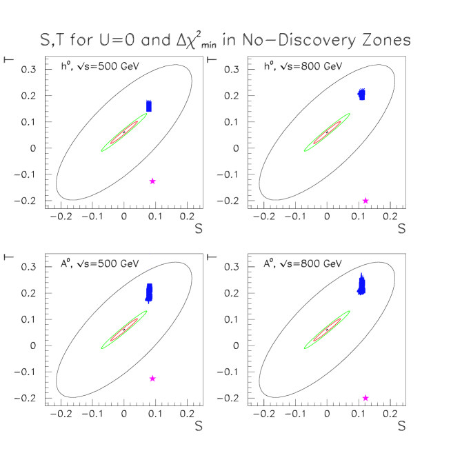
Figure 15: The outer ellipse gives the current 90% CL region for $U=0$ and SM Higgs mass of 115 GeV. The blobs show the $S,T$ predictions for the 2HDM models described in the text that have minimum $\Delta\chi^{2}$ relative to this SM benchmark and for which no Higgs boson of the 2HDM will be detected at the LC. The innermost (middle) ellipse gives the 90% (99.9%) CL region for $m_{h_{\rm SM}}=115{\rm\,GeV}$ obtained after Giga-Z precision measurements and a $\Delta m_{W}\mathrel{\raise 1.29167pt\hbox{$<$\kern-7.5pt\lower 4.30554pt\hbox{$\sim$}}}6$ MeV threshold scan measurement of $m_{W}$. The stars indicate the minimal SM $S,T$ prediction if $m_{h_{\rm SM}}=\sqrt{s}$.

In composite Higgs models with extra fermions, there are similar non-degeneracies of the fermions that can yield a similar positive contribution to $\Delta\rho$ and thence $T$. As reviewed in [13], consistency with current precision electroweak data inevitably constrains parameters so that some type of new physics (including a possible heavy scalar sector) would again have to lie below a TeV or so. Future Giga-Z data could provide much stronger constraints on these types of models, as discussed in Section 9.

3 Constraints on Higgs bosons with $VV$ coupling

In the MSSM, we know that the Higgs boson(s) that carry the $VV$ coupling must be light: if $m_{A^{0}}$ is large (the decoupling limit) then it is the mass-bounded $h^{0}$ that has all the $VV$ coupling strength; if $m_{A^{0}}\mathrel{\raise 1.29167pt\hbox{$<$\kern-7.5pt\lower 4.30554pt\hbox{$\sim$}}}2m_{Z}$, then the $H^{0}$ can share the $VV$ coupling with the $h^{0}$, but then $m_{H^{0}}$ cannot be larger than about $2m_{Z}$. In the NMSSM, assuming Higgs-sector CP conservation, there are 3 neutral CP-even Higgs bosons, $h_{1,2,3}$ ($m_{1}<m_{2}<m_{3}$), which can share the $VV$ coupling strength. One can show (see [67] for a recent update) that the masses of the $h_{i}$ with substantial $VV$ coupling are strongly bounded from above. This result generalizes to the most general supersymmetric Higgs sector as follows. Labeling the neutral Higgs bosons by $i$ with masses $m_{h_{i}}$ and denoting the $ZZ$ squared-coupling relative to the SM by $K_{i}$, it can be shown that

$$\sum_{i}K_{i}\geq 1\,,\quad\sum_{i}K_{i}m_{h_{i}}^{2}\leq(200{\rm\,GeV})^{2}\,.$$ (11)

That is, the aggregate strength of the $VV$ coupling-squared of all the neutral Higgs bosons is at least that of the SM, and the masses-squared of the neutral $h_{i}$ weighted by the coupling-squared must lie below a certain bound. The upper bound of $(200{\rm\,GeV})^{2}$ in Eq. (11) is obtained [41] by assuming that the MSSM remains perturbative up to the the GUT scale of order $10^{19}{\rm\,GeV}$. This bound applies for the most general possible Higgs representations (including triplets) in the supersymmetric Higgs sector and for arbitrary numbers of representations. If only doublet and singlet representations are allowed for, the bound would be lower. The $(200{\rm\,GeV})^{2}$ bound also applies to general Higgs-sector-only extensions of the SM by requiring consistency with precision electroweak constraints and assuming the absence of a large contribution to $T$ from the Higgs sector itself or from new physics, such as discussed in Section 2.

4 Detection of non-exotic extended Higgs sector scalars at the Tevatron and LHC

In the case of extended Higgs sectors, all of the same processes as discussed for the SM and MSSM will again be relevant. However, we can no longer guarantee Higgs discovery at the Tevatron and/or LHC. In particular, if there are many Higgs bosons sharing the $WW,ZZ$ coupling, Higgs boson discovery based on processes that rely on the $VV$ coupling could be much more difficult than in models with just a few light Higgs bosons with substantial $VV$ coupling. This is true even if the sum rule of Eq. (11) applies. For example, at the LHC even the NMSSM addition of a single singlet to the minimal two-doublet structure in the perturbative supersymmetric context allows for parameter choices such that no Higgs boson can be discovered [68] using any of the processes considered for SM Higgs and MSSM Higgs detection. The $\gamma\gamma$ decay channel signals are all weak (because of decreased $W$-loop contribution to the coupling). Further, if a moderate value of $\tan\beta$ is chosen then $t\overline{t}+$Higgs processes are small and $b\overline{b}+$Higgs processes are insufficiently enhanced. In short, the equivalent to the wedge of Fig. 14 enlarges. The $h^{0}$ signal is divided among the three light neutral CP-even Higgs bosons and diluted to too low a statistical significance.

However, in other cases, the Tevatron and LHC could observe signals not expected in an approximate decoupling limit. For example, in the 2HDM model discussed earlier the light $\widehat{h}$ with no $VV$ couplings decays via $\widehat{h}\to b\overline{b},\tau^{+}\tau^{-}$ and discovery in $t\overline{t}\widehat{h}$, $b\overline{b}\widehat{h}$ and even $gg\to\widehat{h}$ [69] is possible, though certainly not guaranteed. Further, in these models there is a heavy neutral Higgs boson having the bulk of the $VV$ coupling and (for consistency with current precision electroweak constraints or with perturbativity) mass $\mathrel{\raise 1.29167pt\hbox{$<$\kern-7.5pt\lower 4.30554pt\hbox{$\sim$}}}1{\rm\,TeV}$. This latter Higgs boson would be detected at the LHC using $gg,WW$ fusion production and $ZZ\to 4\ell,WW\to 2j\ell\nu,\ldots$ decay modes, just like a heavy minimal SM Higgs boson.

5 LC production mechanisms for non-exotic extended Higgs sector scalars

Any physical Higgs eigenstate with substantial $WW$ and $ZZ$ coupling will be produced in Higgsstrahlung and $WW$ fusion at the LC. Although there could be considerable cross section dilution and/or resonance peak overlap, the LC will nonetheless always detect a signal. This has been discussed for the MSSM in Section 4. In the NMSSM, if one of the heavier CP-even $h_{i}$ has most of the $VV$ coupling, the strong bound on its mass [67] noted earlier implies that it will be detected at any LC with $\sqrt{s}>350{\rm\,GeV}$ within a small fraction of a year when running at planned luminosities. The worst possible case is that in which there are many Higgs bosons with $VV$ coupling with masses spread out over a large interval with separation smaller than the mass resolution. In this case, the Higgs signal becomes a kind of continuum distribution. Still, in [70] it is shown that the sum rule of Eq. (11) guarantees that the Higgs continuum signal will still be detectable for sufficient integrated luminosity, $L\mathrel{\raise 1.29167pt\hbox{$>$\kern-7.5pt\lower 4.30554pt\hbox{$\sim$}}}200~{}\mbox{fb${}^{-1}$}$, as a broad excess in the recoil mass spectrum of the $e^{+}e^{-}\to ZX$ process. (In this case, $WW$ fusion events do not allow for the reconstruction of Higgs events independently of the final state Higgs decay channel.) As already noted, the value of $200{\rm\,GeV}$ appearing in Eq. (11) can be derived from perturbative RGE constraints for the most general Higgs sector in supersymmetric theories and is also required by precision electroweak data for general SM Higgs sector extensions, at least in theories that do not have a large positive contribution to $T$ from a non-decoupling structure in the Higgs sector or from new physics not associated with the Higgs sector.

Other production modes of relevance include Higgs pair production, $t\overline{t}+$Higgs, and $b\overline{b}+$Higgs. In multi-doublet models, $t\overline{b}H^{-}$ and $b\overline{t}H^{+}$ reactions are present. However, none of these are guaranteed to be either kinematically accessible or, if accessible, to have a sufficiently high event rate to be observed.

Regardless of the production process, relevant decay channels could include cases where heavier Higgs bosons decay to lighter ones. If observed, such decays would provide vital information regarding Higgs self-couplings.

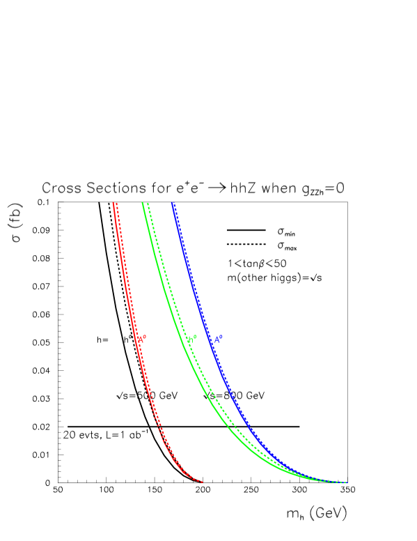
Figure 16: For $\sqrt{s}=500{\rm\,GeV}$ and $800{\rm\,GeV}$ and for $\widehat{h}=h^{0}$ and $\widehat{h}=A^{0}$, we plot as a function of $m_{\widehat{h}}$ the maximum and minimum values of $\sigma(e^{+}e^{-}\to\widehat{h}\widehat{h}Z)$ found after scanning $1<\tan\beta<50$ taking all other higgs masses equal to $\sqrt{s}$. For $\widehat{h}=h^{0}$, we require $\sin(\beta-\alpha)=0$ during the scan. The 20 event level for $L=1000$ fb^-1 is indicated.

We should particularly consider what production processes are most relevant for those Higgs bosons (denoted $\widehat{h}$) that do not have substantial $VV$ coupling. Such processes have particular relevance in the non-decoupling scenario for the general 2HDM model discussed earlier. There, such a $\widehat{h}$ is the only Higgs boson light enough to be produced at an LC with $\sqrt{s}\mathrel{\raise 1.29167pt\hbox{$<$\kern-7.5pt\lower 4.30554pt\hbox{$\sim$}}}1{\rm\,TeV}$ and it cannot be produced and detected in $WW$ fusion or Higgsstrahlung. Since the other Higgs bosons are heavy, the $\widehat{h}$ also cannot be produced in association with another Higgs boson. As shown in [71, 65], the $b\overline{b}\widehat{h}$ and $t\overline{t}\widehat{h}$ processes will also not be detectable at the LC if $\tan\beta$ is moderate in value. The most interesting tree-level processes are then those based on the quartic couplings $WW\widehat{h}\widehat{h}$ and $ZZ\widehat{h}\widehat{h}$ required by gauge invariance [72, 73]. These couplings allow for $WW\to\widehat{h}\widehat{h}$ fusion and $Z^{*}\to Z\widehat{h}\widehat{h}$ production, respectively. The exact cross sections for these processes are only mildly sensitive to the masses of the other heavier Higgs bosons via 2HDM Higgs self-couplings. Of course, phase space restrictions imply an upper limit on the $\widehat{h}$ masses that can be probed in this way. Cross sections in the case of $Z^{*}\to Z{\widehat{h}}{\widehat{h}}$ are plotted in Fig. 16 for both $\widehat{h}=A^{0}$ and $\widehat{h}=h^{0}$ taking $\sqrt{s}=500$ [74]. Assuming optimistically that 20 events in $L=1000~{}\mbox{fb${}^{-1}$}$ could be detected, $Z^{*}\to Z\widehat{h}\widehat{h}$ could be detected for $m_{\widehat{h}}$ as large as $150{\rm\,GeV}$. At $\sqrt{s}=800{\rm\,GeV}$, this limit increases to $250{\rm\,GeV}$. Similar results are obtained for $WW\to\widehat{h}\widehat{h}$ fusion production.

8 Measurements of Higgs boson properties at the LC

The strength of the LC physics program is that it cannot only observe one or more Higgs boson(s), but also precisely determine the Higgs boson mass, width, couplings, and quantum numbers, and parameters of the Higgs potential. These measurements are crucial to establish the nature of the Higgs and thus to illuminate the mechanism of electroweak symmetry breaking. Measurements of the Higgs couplings can demonstrate that a Higgs boson generates the masses of vector bosons, charged leptons, and up- and down-type quarks. If the measured couplings are not simply proportional to mass, this will require a Higgs sector more complex than a single complex Higgs doublet. Accurate measurements are needed to distinguish the SM Higgs and $h^{0}$ of the MSSM near the decoupling limit. Couplings are determined through measurements of Higgs branching ratios and cross sections. Higgs bosons are also expected to couple to themselves, and this self-coupling $\lambda$ can only be explored through the direct production of two or more Higgs bosons. The measurement of direct and model independent absolute Higgs couplings is a major cornerstone of the LC program.

Details of some of the studies of Higgs coupling measurements can be found in [75]. A comprehensive description of European studies using the simulated TESLA detector can be found in [76]. North American studies consider simulations of detectors with capabilities described in Chapter 15. The program of measurements of Higgs boson properties strongly impacts detector design. Measurement of branching ratios into fermions requires sophisticated vertex detectors to separate $b$ from $c$ (and gluon) jets. Precise recoil mass measurements need excellent momentum resolution (particularly for $\mu^{+}\mu^{-}$) from charged particle tracking. The performance of the combined tracking and calorimetry systems needs to result in precise jet-jet invariant masses, missing mass measurements, and the ability to separate hadronic $W$ from hadronic $Z$ decays.

The specific measurements used to determine the Higgs couplings to vector bosons, fermions and scalars are significantly different depending on the mass of the Higgs boson. A generic neutral CP-even Higgs boson will be denoted by $h$ in this section. We treat three cases separately: a light Higgs boson ($m_{h}<2m_{W}$), an intermediate mass Higgs boson ($2m_{W}\leq m_{h}<2m_{t}$), and a heavy Higgs boson ($m_{h}\geq 2m_{t}$).

1 Mass

In the Standard Model, the Higgs mass determines all its other properties. Thus, the precision of the mass measurement affects the comparison of theory and experiment, for example, in a global fit of cross sections, branching ratios, and precision electroweak data. Similarly, in the MSSM or other models with extended Higgs sectors, the masses of all the Higgs bosons are an important input in determining the underlying model parameters.

For this fundamental mass measurement, a LC can reconstruct the system recoiling against a $Z$ (independent of Higgs decay). Full event reconstruction, plus kinematic constraints, can improve resolution and clean up mass tails. For a light or intermediate mass Higgs boson, the optimal running conditions would have a smaller center-of-mass energy such as $\sqrt{s}=350$ GeV, to allow better momentum resolution and to minimize the beamstrahlung. Under such conditions, one can precisely measure the recoil mass in $e^{+}e^{-}\rightarrow Zh$ events opposite to the reconstructed leptonic decay $Z\rightarrow e^{+}e^{-}$ or $\mu^{+}\mu^{-}$. This measurement is independent of the Higgs decay mode. Accuracy can be improved by reconstructing specific decay modes, leading, for example, to a four-jet topology where effective (5-C) kinematic constrained fits can be employed.

Figure 17 shows the distribution of the recoil mass,

$$M_{\rm recoil}=\sqrt{s-2\sqrt{s}\cdot E_{\ell^{+}\ell^{-}}+M^{2}_{\ell^{+}\ell^{-}}}\,,$$ (12)

in a simulation of the L linear collider detector [77] described in Chapter 15 for Higgs masses between 115 and 160 GeV [78]. Using Monte Carlo shape templates and an integrated luminosity of 500 fb^-1, precisions of $\Delta m_{h_{\rm SM}}\simeq 80$ MeV at $\sqrt{s}=350$ GeV and $\Delta m_{h_{\rm SM}}\simeq 140$ MeV at $\sqrt{s}=500$ GeV have been estimated for either the $e^{+}e^{-}$ or $\mu^{+}\mu^{-}$ mode.

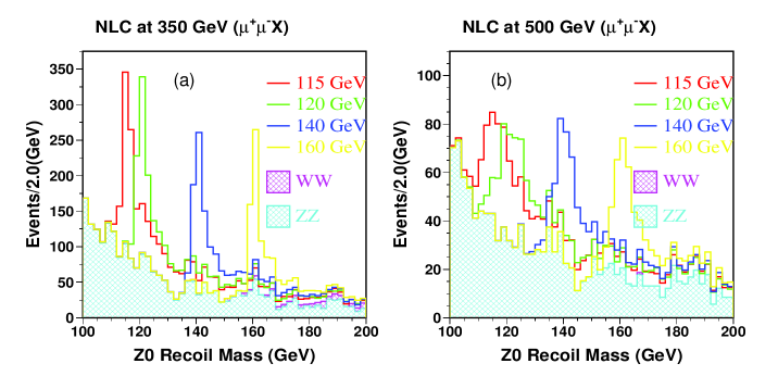
Figure 17: Recoil mass from a pair of leptons for different Higgs masses at (a) $\sqrt{s}=350$ GeV and (b) 500 GeV simulated in the L detector described in Chapter 15.

Realistic simulations have also been made with the L detector for the process $Zh\rightarrow q\overline{q}h$ resulting in four jets. Figure 18(a) shows the jet-jet invariant mass distribution for pairs of jets for Higgs with $m_{h_{\rm SM}}=115$ GeV recoiling against a $Z$ reconstructed from its hadronic decay mode [79]. A clean Higgs signal with a mass resolution of approximately 2 GeV is observed. The central Higgs mass is shifted down by the loss of low-energy charged and neutral particles in the simulated event reconstruction. A low-mass tail of the Higgs signal arises from missing neutrinos in semi-leptonic $b$ and $c$ quark decays. Using neural net tags and full kinematic fitting [80], the mass peak shown in Fig. 18(b) is obtained for $m_{h_{\rm SM}}=120$ GeV, $\sqrt{s}=500$ GeV, and 500 fb^-1 resulting in $\Delta m_{h_{\rm SM}}\simeq 50$ MeV. If a second lower-energy IR is available, it might be attractive to perform a scan across the $Zh$ threshold. With a total integrated luminosity of 100 fb^-1, $\Delta m_{h_{\rm SM}}\simeq 100$ MeV at $m_{h_{\rm SM}}=150$ GeV is achievable [81], competitive with the methods above.

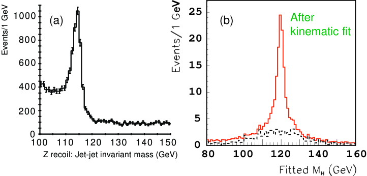
Figure 18: (a) Jet-jet invariant mass of the jets recoiling from a $Z$ reconstructed hadronically simulated in the LCD Large detector, $m_{h_{\rm SM}}=115$ GeV. (b) Direct reconstruction of the four-jet $q\overline{q}h_{\rm SM}$ state simulated in the L detector after fitting with full kinematic constraints, $m_{h_{\rm SM}}=120$ GeV.

Further work is necessary to confirm analogous precisions for heavier Higgs bosons and MSSM Higgs bosons with different decay modes and possible close mass-degeneracies. The number of $Zh$ events with $Z\rightarrow\ell^{+}\ell^{-}$ for an intermediate-mass ($m_{h}>2m_{W}$) or heavy Higgs ($m_{h}>2m_{t}$) with SM coupling falls quickly [82]. In this case, and for the decays $h\rightarrow ZZ$, hadronic decays of the $Z$ would have to be considered to gain sufficient statistics. For the heavier MSSM Higgs boson states, European studies [83] have shown typical mass precisions of $\Delta m_{H^{\pm}}$ and $\Delta m_{A^{0},H^{0}}$ of around 1 GeV for 500 fb^-1, but at $\sqrt{s}=800$ GeV. The MSSM $H^{0}$ and $A$ may be studied separately using $\gamma\gamma\rightarrow H/A$ with different states of $\gamma$ linear polarization, thus helping to refine mass determinations in the nearly degenerate case.

2 Coupling determinations—light Higgs bosons

Cross sections

For Higgs masses below $2m_{W}$, the couplings $g_{hZZ}$ and $g_{hWW}$ are best measured through measurements of the Higgsstrahlung and $WW$ fusion cross sections, respectively. These cross sections are also critical in the extraction of branching ratios since the experimental measurement will be a product of cross section and branching ratio.

Measurement of the cross section $\sigma(Z^{*}\rightarrow Zh)$ is best addressed via the recoil mass method outlined above [78]. Again, in this case, to reduce the contribution from the $WW$ fusion process, it may be preferrable to run at a lower energy, i.e., $\sqrt{s}=350$ GeV, and to examine recoil against $\mu^{+}\mu^{-}$ to avoid large Bhabha backgrounds. The study with the L detector described above finds $\Delta\sigma/\sigma\simeq 4$% at $\sqrt{s}=350$ GeV and $\simeq$6.5% at 500 GeV with 500 fb^-1 as shown in Fig. 19(a). These agree roughly with estimates from European studies [84].

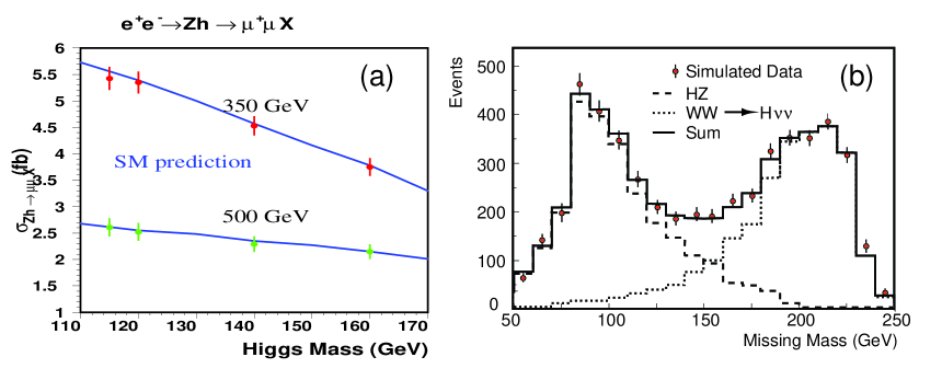
Figure 19: (a) Cross section measurement for 500 fb^-1 and (b) separation of Higgsstrahlung and $WW$ fusion ($\sqrt{s}=350$ GeV) through a fit (after background subtraction), both simulated in the L detector.

With efficient and pure $b$-jet tagging, events due to $e^{+}e^{-}\rightarrow W^{+}W^{-}\nu\overline{\nu}\rightarrow\nu\overline{\nu}h\rightarrow\nu\overline{\nu}b\overline{b}$ can be separated from those due to Higgsstrahlung, $Zh\rightarrow\nu\overline{\nu}h\rightarrow\nu\overline{\nu}b\overline{b}$ by examining the missing mass distribution and fitting to the expected shapes of a peak at $m_{Z}$ from Higgsstrahlung and the higher missing masses from $WW$ fusion. This technique has been confirmed with simulations of the L detector as shown in Fig. 19(b) [85]. With 500 fb^-1 and a precision $\mbox{\rm BR}(h_{\rm SM}\rightarrow b\overline{b})\simeq 3$% (see below), the fusion-process cross section with this analysis can be found with a precision $\Delta\sigma/\sigma$ = 3.5% for $m_{h_{\rm SM}}=120$ GeV.

Branching ratios

A key advantage of the linear collider in Higgs studies is the identification of Higgsstrahlung $Zh$ events through the tag of the $Z$ decays. This selection is essentially independent of the decay mode of the $h$ and simplifies the measurement of Higgs boson branching ratios.

Small beam sizes, the possibility of a first track measurement as close as 1 cm from the beam axis, and sophisticated pixel vertex detectors allow for efficient and clean separation of quark flavors. Separate tagging of $b$, $c$ and $g$ jets is possible.

In a study [86] of vertexing using a CCD vertex detector in a standard LC detector configuration (C1 in [87]), topological vertexing [88] with neural net selection was used for flavor (or anti-flavor, i.e., $WW^{*}$) tagging. The separation of $b\overline{b}$ and $c\overline{c}$ events by this method is illustrated in Fig. 21(a). Assuming 500 fb^-1 and 80% polarization, the results shown in Table 1 were obtained.

	$m_{h_{\rm SM}}=120$ GeV		$m_{h_{\rm SM}}=140$ GeV
	BR	$\delta\mbox{\rm BR}/\mbox{\rm BR}$	BR	$\delta\mbox{\rm BR}/\mbox{\rm BR}$
$h_{\rm SM}\rightarrow b\overline{b}$	$(69\pm 2.0)$%	2.9%	$(34\pm 1.3)$%	4.1%
$h_{\rm SM}\rightarrow WW^{*}$	$(14\pm 1.3)$%	9.3%	$(51\pm 1.8)$%	3.7%
$h_{\rm SM}\rightarrow c\overline{c}$	$(2.8\pm 1.1)$%	39%	$(1.4\pm 0.64)$%	45%
$h_{\rm SM}\rightarrow gg$	$(5.2\pm 0.93)$%	18%	$(3.5\pm 0.79)$%	23%
$h_{\rm SM}\rightarrow\tau^{+}\tau^{-}$	$(7.1\pm 0.56)$%	7.9%	$(3.6\pm 0.38)$%	10%

Table 1: Predicted branching ratio precisions in the L detector and typical vertex detector configuration for 500 fb^-1 and $\sqrt{s}=500$ GeV.

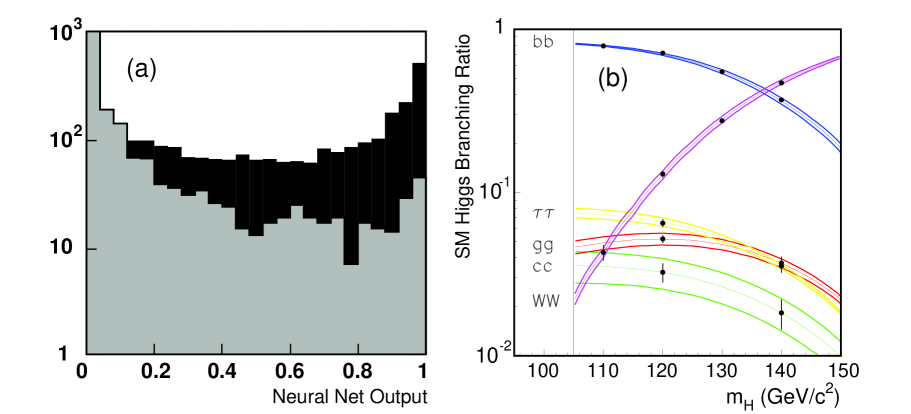
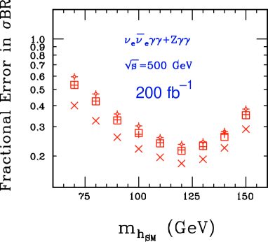
Figure 20: (a) For the simulated L detector with CCD vertex detector, neural net $h_{\rm SM}\rightarrow c\overline{c}$ output for $h_{\rm SM}\rightarrow c\overline{c}$ events (dark) compared to output for $h_{\rm SM}\rightarrow b\overline{b}$ events (gray). (b) Variation of branching ratios with SM Higgs mass (bands are 1$\sigma$ uncertainties on the theoretical predictions) and measurement precisions in the TESLA detector (points with error bars).

Figure 21: Fractional error on the branching ratio $\mbox{\rm BR}(h_{\rm SM}\rightarrow\gamma\gamma)$. The open squares are for a typical LC detector electromagnetic energy resolution of $\Delta E/E=10\%/\sqrt{E}\oplus 1.0\%$.

These results scale approximately as $(\sigma\int{\cal L}dt)^{-1/2}$ when taken together with other studies [89, 90, 91], but the results of [91] (shown in Fig. 21(b)) are noticeably more precise for the $c\overline{c}$ and $gg$ modes. These branching ratio measurements can then be used to either distinguish a SM Higgs boson from an MSSM Higgs boson, or to probe higher-mass states and extract MSSM parameters such as $m_{A^{0}}$ even if the CP-odd $A^{0}$ is not accessible. That analysis is described in more detail below.

An accessible decay mode for lighter Higgs bosons is $h\rightarrow\gamma\gamma$, which requires excellent electromagnetic calorimetry. As shown in Fig. 21, for a SM Higgs boson in a typical LC detector, this is a difficult measurement requiring a large luminosity, which is best optimized for masses around 120 GeV [92]. A higher-luminosity study [93] with 1000 fb^-1 and $m_{h_{\rm SM}}=120$ GeV for the TESLA detector finds $\delta\mbox{\rm BR}/\mbox{\rm BR}=14$%. A $\gamma\gamma$ collider, discussed in Section 10, would be a more powerful tool for determining the Higgs coupling to photons.

For light Higgs bosons, the coupling to top quarks is still accessible via the radiative process $t\overline{t}h$ described below, or indirectly through $\mbox{\rm BR}(h\rightarrow gg)$.

A set of difficult decay channels for the LHC is invisible decays of the Higgs boson into, e.g., neutralinos, majorans or heavy neutrinos. The LC can close this loophole and measure the branching ratio easily, even for branching ratios as small as 5% for a relatively narrow Higgs state, by using the recoil mass method and demanding no detector activity opposite the $Z$, or by comparing the number of events tagged with $Z\rightarrow\ell^{+}\ell^{-}$ with the total number of observed Higgs decays into known states.

Radiative production and $t\overline{t}h$ coupling

For a light Higgs boson, production through radiation off a top quark is feasible, resulting in a final state of $t\overline{t}h$ . This allows a determination of the Yukawa top quark coupling $g_{htt}$ [23, 24]. For a SM-like Higgs boson with $m_{h}=120$ GeV, the $t\overline{t}h$ cross section is roughly 10 times larger at $\sqrt{s}=700$–800 GeV than at 500 GeV. At $\sqrt{s}=800$ GeV, a statistical error of $\delta g_{htt}/g_{htt}\sim 5\%$ was estimated [94] for $L=500~{}\mbox{fb${}^{-1}$}$ on the basis of an optimal observable analysis. At $\sqrt{s}=500$ GeV, a statistical error of $\delta g_{htt}/g_{htt}\simeq 21$% is estimated [95] using 1000 fb^-1. A more sophisticated analysis using neural net selections, full simulation, and the same integrated luminosity at $\sqrt{s}=800$ GeV finds a total error of 6% on the coupling [96]. More details on this process can be found in Chapter 6, Section 3.1.

Higgs self-coupling

To delineate the Higgs sector fully, it is essential to measure the shape of the Higgs potential. The cross section for double Higgs production (e.g., $Zhh$) is related to the triple Higgs coupling $g_{hhh}$, which in turn is related to the spontaneous symmetry breaking shape of the Higgs potential. The Higgs mass, $m_{h}^{2}=4\lambda v^{2}$, also measures the potential shape parameter $\lambda$, so independent determinations through $hh$ production give a cross-check. In the MSSM, a variety of double Higgs production processes would be required to determine $g_{h^{0}h^{0}h^{0}}$, $g_{A^{0}h^{0}h^{0}}$, etc. [73].

These cross sections are low, and high integrated luminosity is needed, bolstered by polarization and neural net selections. Experimental studies [97, 98] indicate that for a SM-like Higgs boson with $m_{h}=120$ GeV at $\sqrt{s}=500$ GeV and 1000 fb^-1, a precision of $\delta g_{hhh}/g_{hhh}=23$% is possible. Regions of accessibility in MSSM parameters for MSSM Higgs self-couplings have also been determined [99, 100].

The cross section for SM triple Higgs production is very low, $\sigma(Zhh)<10^{-3}$ fb, so measurement of the quartic coupling $g_{hhhh}$ is hopeless with currently envisioned luminosities.

Implications for the MSSM Higgs sector

The discussion of light Higgs coupling determinations has been based on the assumption that the actual Higgs couplings to fermions, vector bosons and scalars are close to the corresponding Standard Model expectations. In Section 1, it was argued that such an expectation is rather generic, and applies to the decoupling limit of models of Higgs physics beyond the Standard Model. In particular, the decoupling limit of the MSSM Higgs sector sets in rather rapidly once $m_{A^{0}}\mathrel{\raise 1.29167pt\hbox{$>$\kern-7.5pt\lower 4.30554pt\hbox{$\sim$}}}150$ GeV [see Section 1]. Since $m_{h^{0}}\mathrel{\raise 1.29167pt\hbox{$<$\kern-7.5pt\lower 4.30554pt\hbox{$\sim$}}}135$ GeV in the MSSM [Eq. (2)], the precision study of $h^{0}$ using the techniques discussed above can distinguish between $h^{0}$ and $h_{\rm SM}$ with a significance that depends on how close the model is to the decoupling limit. Said another way, the detection of deviations in the Higgs couplings from their Standard Model predictions would yield evidence for the existence of the non-minimal Higgs sector, and in the context of the MSSM would provide constraints on the value of $m_{A^{0}}$ (with some dependence on $\tan\beta$ and other MSSM parameters that enter in the Higgs radiative corrections).

In [101], the potential impact of precision Higgs measurements at the LC on distinguishing $h^{0}$ from $h_{\rm SM}$ was examined. The fractional deviation of the $h^{0}$ branching ratios into a given final state from the corresponding result for $h_{\rm SM}$ (assuming the same Higgs mass in both cases) is defined as:

$$\delta\mbox{\rm BR}=\frac{\mbox{\rm BR}_{\rm MSSM}-\mbox{\rm BR}_{\rm SM}}{\mbox{\rm BR}_{\rm SM}}.$$ (13)

For the MSSM Higgs boson decay, both $m_{h^{0}}$ and the corresponding branching ratios were computed including the radiative corrections due to the virtual exchange of Standard Model and supersymmetric particles, as described in Section 2. Thus, the $h^{0}$ branching ratios depend on $m_{A^{0}}$ and $\tan\beta$ (which fix the tree-level MSSM Higgs sector properties) and a variety of MSSM parameters that govern the loop corrections. Four scenarios were considered: the minimal and maximal top-squark mixing cases [see Eq. (2) and surrounding text], and two additional cases with large $|\mu|=|A_{t}|$ (for $\mu A_{t}<0$ and two possible sign choices of $\mu$), where $\mu$ and $A_{t}$ control the top-squark mixing. In the latter two scenarios, significant renormalization of the CP-even Higgs mixing angle $\alpha$ and $\Delta_{b}$ [see Eq. (2)] can arise.

In Fig. 22, contours of $\delta\mbox{\rm BR}$ are plotted for three $h^{0}$ decay modes: $b\overline{b}$, $WW^{*}$ and $gg$. The contours shown correspond roughly to the $1\sigma$ and $2\sigma$ measurements claimed by [91], rescaled for the LC at $\sqrt{s}=500$ GeV (see also the $b\overline{b}$ and $WW^{*}$ branching ratio precisions given in Table 1). In the minimal and maximal scenarios, the dependence on $m_{A^{0}}$ is nearly independent of $\tan\beta$, and demonstrates that one can achieve sensitivity to values of $m_{A^{0}}$ that lie significantly beyond $\sqrt{s}/2$ where direct production at the LC via $e^{+}e^{-}\to H^{0}A^{0}$ is kinematically forbidden. However, the cases with large $|\mu|=|A_{t}|$ exhibit the possibility of “premature” decoupling, that is, relatively low values of $m_{A^{0}}$ (at a particular large value of $\tan\beta$) at which the properties of $h^{0}$ and $h_{\rm SM}$ cannot be distinguished by the decay modes considered above. Thus, a measured deviation of Higgs branching ratios that distinguishes $h^{0}$ from $h_{\rm SM}$ can place significant constraints on the heavier non-minimal Higgs states, although the resulting constraints can depend in a nontrivial way on the value of the MSSM parameters that control the Higgs radiative corrections.

Figure 22: Contours of $\delta\mbox{\rm BR}(b\overline{b})=3$ and 6% (solid), $\delta\mbox{\rm BR}(WW^{*})=8$ and 16% (dashed) and $\delta\mbox{\rm BR}(gg)=8$ and 16% (dotted) [BR deviations defined in Eq. (13)] in the no (i.e. minimal) mixing scenario (top left), the maximal mixing scenario (top right), and the large $\mu$ and $A_{t}$ scenario with $\mu=-A_{t}=1.2$ TeV (bottom left) and $\mu=-A_{t}=-1.2$ TeV (bottom right). Taken from [101].

3 Coupling determinations—intermediate mass Higgs bosons

For $m_{h}<2m_{W}$, the measurement of branching ratios is extremely rich, yielding couplings to both many of the fermions and bosons. For larger masses, decays to $f\overline{f}$ become rarer until the threshold for decays into top is crossed. In this intermediate mass range, a LC can measure the $W$ and $Z$ couplings more precisely than the LHC both through Higgs production rates and via branching ratios for decays into these bosons. Whether the observed Higgs boson fully generates the $W$ and $Z$ mass can then be checked.

Precision electroweak measurements in the framework of the Standard Model indirectly predict [8, 9] $m_{h_{\rm SM}}\mathrel{\raise 1.29167pt\hbox{$<$\kern-7.5pt\lower 4.30554pt\hbox{$\sim$}}}205$–230 GeV at 95% CL, and a Higgs observed with mass much greater than this would imply new physics. At this point, measurements from a Giga-Z dataset would be particularly useful to probe this new sector.

Cross sections

Techniques described earlier [78, 85] for cross section measurements of both the Higgsstrahlung and $W$-fusion processes, with subsequent Higgs decays into $b\overline{b}$, can still be used for the lower portion of the intermediate mass range, i.e., $m_{h}\sim 160$ GeV. Even in this intermediate mass range, it is beneficial to run at the peak of the cross section at roughly $m_{h}+m_{Z}+50$ GeV. The typical precisions that can be obtained are $\Delta\sigma(Zh_{\rm SM})/\sigma(Zh_{\rm SM})\simeq 5$% and $\Delta\sigma(\nu\overline{\nu}h_{\rm SM})/\sigma(\nu\overline{\nu}h_{\rm SM})\simeq 17$% for $m_{h_{\rm SM}}=160$ GeV, at $\sqrt{s}=350$ GeV with 500 fb^-1.

For heavier Higgs bosons in this mass range, cross sections for both Higgsstrahlung and $W$-fusion will need to be extracted from using the decay $h\rightarrow WW^{*}$, for example, as described in [90]. Couplings determined from $t\overline{t}h$ and $Zhh$ production would clearly need higher $\sqrt{s}$.

Branching ratios

Using Higgsstrahlung events at an optimal $\sqrt{s}$, the statistical error on $\mbox{\rm BR}(h_{\rm SM}\rightarrow b\overline{b})$ is still only 6.5% at $m_{h_{\rm SM}}=160$ GeV [91]. At $\sqrt{s}=500{\rm\,GeV}$, with leptonic decays of the $Z$ only, the statistical error on this branching ratio reaches 25% at $m_{h_{\rm SM}}\simeq 165$ GeV with 250 fb^-1 and remains below 30% for $m_{h_{\rm SM}}<200$ GeV with 2000 fb^-1 [82]. However, in addition to the leptonic decays of the $Z$, hadronic decays can also be used to tag the associated $Z$. Extrapolating from full LCD detector simulations, it is conservatively estimated that including the hadronic decays of the $Z$ results in an increase in signal statistics above background by a factor of four. With these assumptions and 500 fb^-1, again with the optimal $\sqrt{s}\simeq 350$ GeV, the error on the $b\overline{b}$ branching ratio can then be estimated to reach 25% at $m_{h_{\rm SM}}\simeq 200$ GeV. Measurement of branching ratios to $c\overline{c}$, $\tau^{+}\tau^{-}$, $gg$, and $\gamma\gamma$ does not seem feasible in this mass range.

Branching ratios into vector bosons can be measured with good precision in the intermediate mass range. For $m_{h_{\rm SM}}=160$ GeV and 500 fb^-1, a predicted excellent precision of 2.1% on $\mbox{\rm BR}(h_{\rm SM}\rightarrow WW)$, has been reported [90], with extrapolated estimated precision of better than 7% over the mass range of 150 to 200 GeV [82].

To measure $\mbox{\rm BR}(h\rightarrow ZZ)$, it will be necessary to distinguish hadronic $Z$ decays from hadronic $W$ decays. This serves as an important benchmark for electromagnetic and hadronic calorimetry. With 500 fb^-1, and assuming that this separation allows one to identify one of the two $Z$’s in the Higgs decays (through leptons or $b\overline{b}$) 40% of the time, the statistical uncertainty of this branching ratio would be approximately 8% for $m_{h_{\rm SM}}\simeq 210$ GeV [82], degrading to 17% for $m_{h_{\rm SM}}=160$ GeV [76] where the branching ratio into $Z$’s is still small.

4 Coupling determinations—heavy Higgs bosons

If the Higgs boson is heavy, i.e., $m_{h}>2m_{t}$, and if this Higgs boson possesses couplings close to those expected in the SM, then consistency with the precision electroweak data (which implies $m_{h_{\rm SM}}\mathrel{\raise 1.29167pt\hbox{$<$\kern-7.5pt\lower 4.30554pt\hbox{$\sim$}}}230$ GeV at 95% CL) would require the existence of new physics beyond the SM. A high statistics measurements at the $Z$ peak could be useful to elucidate the non-SM effects. In addition, with high center of mass energy and large integrated luminosity, an experiment at the LC could directly observe heavy Higgs decay and make measurements of the Higgs couplings. These measurements could reveal departures from the SM Higgs properties and provide indirect evidence for the nature of the new physics, which would modify the SM Higgs couplings through loop effects.

Cross sections

As a specific case, for $m_{h}=500$ GeV, a SM-like Higgs boson would have a width of 70 GeV and dominant decay modes into $W^{+}W^{-}$ (55%), $ZZ$ (25%), and $t\overline{t}$ (20%). The production cross section at $\sqrt{s}=800$ GeV for $Zh$ would be 6 fb, but Higgs production would be dominated by the $W$-fusion process, whose cross section would be 10 fb. With 1000 fb^-1, one would expect 400 $Zh$ events where the $Z$ decays to electrons or muons. With reasonable selection and acceptance cuts, a measurement of $\sigma(Zh)$ to better than 7% should be feasible.

Branching ratios

The LHC will have great difficulty distinguishing $h\rightarrow t\overline{t}$ decays from the huge QCD $t\overline{t}$ backgrounds. On the other hand, this mode should be observable at a LC. In the SM, the important coupling $g^{2}_{tth_{\rm SM}}\simeq 0.5$ can be compared to $g^{2}_{bbh_{\rm SM}}\simeq 4\times 10^{-4}$. If the Higgs boson is heavier than 350 GeV, it will be possible obtain a good determination of the top-Higgs Yukawa coupling. Full simulations are needed for heavy Higgs decays into top, but with reasonable assumptions, one can expect a statistical error of $\delta\mbox{\rm BR}/\mbox{\rm BR}\simeq 14$% with 500 fb^-1 [82]. Simulations using the TESLA detector of the $W^{+}W^{-}\rightarrow h_{\rm SM}\rightarrow t\overline{t}$ process with 1000 fb^-1 and 6-jet final states show impressive signal significance for $\sqrt{s}=1000$ GeV and reasonably good significance at $\sqrt{s}=800$ GeV [102]. These studies find that a relative error of better than 10% in the top quark Yukawa coupling measurement can be achieved for Higgs masses in the 350–500 GeV and 350–650 GeV ranges at $\sqrt{s}=800$ GeV and 1000 GeV, respectively.

Assuming that detector performance allows separation of hadronic $W$ and $Z$ decays, and using production through $W$-fusion, the $WW$ and $ZZ$ coupling of the Higgs boson can be studied by using methods similar to those for $t\overline{t}$. This gives the estimates on $\mbox{\rm BR}(h_{\rm SM}\rightarrow W^{+}W^{-})$ and $\mbox{\rm BR}(h_{\rm SM}\rightarrow ZZ)$ shown in Table 2.

5 Summary of couplings

The relative measurement errors for a SM Higgs at various masses are summarized in Table 2. As much as possible, the entries have been collected from simulations with the L detector described in Chapter 15. For uniformity, the entries have been scaled to 500 fb^-1, except where otherwise noted. The significant measurements of many branching ratios and couplings demonstrate the strength of the LC Higgs program.

$\Delta m_{h}$	$\simeq 140$ MeV (recoil against leptons from $Z$)
	$\simeq 50$ MeV (direct reconstruction)
$m_{h}$ (GeV)	120	140	160	200	400–500
$\sqrt{s}$ (GeV)	500				800
$\Delta\sigma(Zh)/\sigma(Zh)$	$6.5$%	$6.5$%	$6$%	$7$%	$10$%
$\Delta\sigma(\nu\overline{\nu}h)\mbox{\rm BR}(b\overline{b})/\sigma\mbox{\rm BR}$	$3.5$%	$6$%	$17$%	–	–
$\delta g_{hxx}/g_{hxx}$ (from BR’s)
$t\overline{t}$	7 – 20% †	–	–	–	10%
$b\overline{b}$	$1.5$%	$2$%	$3.5$%	$12.5$%	–
$c\overline{c}$	$20$%	$22.5$%	–	–	–
$\tau^{+}\tau^{-}$	$4$%	$5$%	–	–	–
$WW^{(*)}$	$4.5$%	$2$%	$1.5$%	$3.5$%	$8.5$%
$ZZ^{(*)}$	–	–	$8.5$%	$4$%	$10$%
$gg$	$10$%	$12.5$%	–	–	–
$\gamma\gamma$	$7$%	$10$%	–	–	–
$g_{hhh}$	$23$% §	–	–	–	–

Table 2: Summary of measurement precisions for the properties of a SM-like Higgs boson, $h$, and couplings for a range of Higgs boson masses for 500 fb^-1, unless otherwise indicated. † radiative $t\overline{t}h$ production, 1000 fb^-1, $\sqrt{s}=800$ – 1000 GeV; § 1000 fb^-1.

Just as the computer program ZFITTER [103] is used with $Z$ mass, widths, asymmetries and branching ratios to make global fits for $Z$ couplings, a program HFITTER [104] is now available that performs a global fit taking into account correlations between measurements of Higgs boson properties. Individual couplings of the Higgs boson can then be extracted optimally, for example through the correct combination of cross section and branching ratio measurements for such couplings as $g_{hWW}$ and $g_{hZZ}$. Such precision fits can be used to probe for indirect evidence of higher-mass states.

6 Total width

Determination that a Higgs boson total width is anomalously large would indicate new non-SM effects. For light Higgs bosons, the predicted SM width is too small to be measured directly, but a combination of branching ratios and coupling measurements allows the indirect and model-independent measurement of the total width through

$$\Gamma_{tot}=\Gamma(h\rightarrow X)/\mbox{\rm BR}(h\rightarrow X)\,.$$ (14)

For $m_{h_{\rm SM}}<115$ GeV, the total width measurement would very likely require a $\gamma\gamma$ collider, an $e^{+}e^{-}$ LC, and input from the LHC [2]. However, limits from LEP2 indicate $m_{h_{\rm SM}}\mathrel{\raise 1.29167pt\hbox{$>$\kern-7.5pt\lower 4.30554pt\hbox{$\sim$}}}115$ GeV and therefore a significant branching ratio to $WW^{*}$. This gives the attractive prospect of a model-independent measurement of the total width using LC measurements alone.

First, measurements of $\sigma(h\nu\nu)\cdot\mbox{\rm BR}(h\rightarrow b\overline{b})$ and $\mbox{\rm BR}(h\rightarrow b\overline{b})$, through recoil Higgsstrahlung measurements, give $\Gamma(h\rightarrow WW^{*})$. Then, a similar independent measurement of $\mbox{\rm BR}(h\rightarrow WW^{*})$ gives the total width, through the relation $\Gamma_{tot}=\Gamma(h\rightarrow WW^{*})/\mbox{\rm BR}(h\rightarrow WW^{*})$. For example, from Table 2, even with as little as 200 fb^-1, $\Gamma_{tot}$ can be found to approximately 10% for $m_{h_{\rm SM}}=120$ GeV, improving to a few percent for $m_{h_{\rm SM}}=150$ GeV. Even better precision can be attained with the introduction of some model assumptions in the value used for $\Gamma(h_{\rm SM}\rightarrow WW^{*})$, e.g., assuming the SU(2) relation between $W$ and $Z$ couplings along with $\sigma_{meas}(Zh_{\rm SM})$.

For $m_{h_{\rm SM}}\mathrel{\raise 1.29167pt\hbox{$>$\kern-7.5pt\lower 4.30554pt\hbox{$\sim$}}}205$ GeV, $\Gamma_{tot}(h_{\rm SM})$ exceeds 2 GeV, and the physical width would be directly resolvable with typical LC detector resolutions. References [2, 105] track these variations of precision for indirect and direct measurements for different values of $m_{h_{\rm SM}}$ and inputs from different machines. The jet-jet mass resolution assumed in [2] has been verified by full simulations [79] in the L detector with 200 fb^-1 of data, resulting in estimated direct measurements of the total width whose accuracy reaches a minimum value of 6% in the mass range of 240–280 GeV. The indirect determination described above can also be pursued, and the combination would allow even better precision.

7 Quantum numbers

The spin, parity, and charge conjugation quantum numbers $J^{PC}$ of a Higgs boson, generically denoted by $\phi$ in this subsection, can potentially be determined in a model-independent way. Useful ingredients include the following:

• A Higgs boson produced in $\gamma\gamma$ collisions cannot have $J=1$ and must have positive $C$ [106].

• The behavior of the $Z\phi$ Higgsstrahlung cross section at threshold constrains the possible values of $J^{PC}$ of the state. If the spin of the $\phi$ is 2 or less, a cross section growing as $\beta$ indicates a CP-even object, whereas a cross section growing as $\beta^{3}$ signals a CP-odd state [107], as shown in Fig. 23(a).

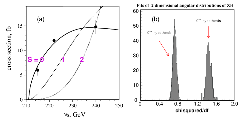
Figure 23: (a) Behavior of Higgsstrahlung threshold for various spin states along with typical measurement precisions on the cross section. (b) Fit to the double-differential angular distribution in $Z\phi$ events (see text) to distinguish CP-even and CP-odd states.

• The angular dependence of the $e^{+}e^{-}\to Z\phi$ cross section depends upon whether the $\phi$ is CP-even, CP-odd, or a mixture [107, 108, 109, 110]. Following [110] we parameterize the $ZZ\phi$ vertex as

  $$\Gamma_{\mu\nu}(k_{1},k_{2})=ag_{\mu\nu}+b\frac{k_{1\mu}k_{2\nu}-g_{\mu\nu}k_{1}\cdot k_{2}}{m_{Z}^{2}}+\tilde{b}\frac{\epsilon_{\mu\nu\alpha\beta}k_{1}^{\alpha}k_{2}^{\beta}}{m_{Z}^{2}}\,,$$ (15)

  where $k_{1}$ and $k_{2}$ are the momenta of the two $Z$s. The first term arises from a Standard-Model-like $ZZ\phi$ coupling, and the last two from effective interactions that could be induced by high-mass virtual particles. With this vertex the Higgsstrahlung cross section becomes

  $$\frac{d\sigma}{d\cos\theta_{Z}}\propto 1+\frac{p_{Z}^{2}}{m_{Z}^{2}}\sin^{2}\theta_{Z}-4\,{\rm Im}\left[\tilde{b}\over\tilde{a}\right]\frac{v_{e}a_{e}}{v_{e}^{2}+a_{e}^{2}}\frac{p_{z}\sqrt{s}}{m_{Z}^{2}}\cos\theta_{Z}+\left|\tilde{b}\over\tilde{a}\right|^{2}\frac{p^{2}_{z}s}{2m_{Z}^{4}}(1+\cos^{2}\theta_{Z})\,,$$ (16)

  where $\theta_{Z}$, $p_{Z}$, and $E_{Z}$ are the scattering angle, momentum, and energy of the final-state $Z$ boson; $v_{e}$ and $a_{e}$ are the vector and axial-vector couplings at the $e^{+}e^{-}Z$ vertex; and $\tilde{a}\equiv a-bE_{Z}\sqrt{s}/m_{Z}^{2}$. The term in Eq. (16) proportional to $\cos\theta_{Z}$ arises from interference between the CP-even and CP-odd couplings in Eq. (15). If the CP-odd coupling $\tilde{b}$ is large enough, it can be extracted from the forward-backward asymmetry. Even upper limits on this asymmetry would be interesting. Note that the CP-even component of a Higgs boson will typically couple at tree-level whereas the CP-odd component will only couple via one-loop diagrams (typically dominated by the $t$ quark loop). As a result the coupling strength $\tilde{b}$ is typically proportional to $m_{Z}^{2}/s$ times a loop suppression factor. Thus, an asymmetry measurement may be able to provide a crude determination of the $\tilde{b}/a$ term. If $\phi$ is a purely CP-odd state with one-loop coupling, the resulting $ZA^{0}$ cross section will simply be too small to provide a useful measurement of the asymmetry.

• The angular distribution of the fermions in the $Z\to f\overline{f}$ decays in $Z\phi$ production also reflects the CP nature of the state $\phi$ [108, 109]. For the decay $Z\rightarrow e^{+}e^{-}$ or $\mu^{+}\mu^{-}$, the following angles can be defined: the angle between the initial $e^{-}$ and the $Z$; the angle between the final state $e^{-}$ or $\mu^{-}$ and the direction of motion of the $Z$, in the rest frame of the $Z$; and the angle between the $Z$ production plane and $Z$ decay plane. Correlations between these angles can be exploited, e.g., a fit to the double-differential angular distribution of the first two of these angles results in a 14$\sigma$ separation between the $0^{++}$ (CP-even, scalar) and the $0^{-+}$ (CP-odd, pseudoscalar) [82], assuming that the $Z\phi$ cross section is independent of the CP nature of $\phi$ (see Fig. 23(b)). Even more powerful are fits to the triple-differential angular distribution, where sufficient luminosity can uncover non-standard $ZZ\phi$ couplings. However, this technique again suffers from the difficulty described in the previous item; namely, the CP-odd part of the state $\phi$ is typically so weakly coupled to $ZZ$ that there is little sensitivity to the CP-odd component if there is any significant CP-even component in $\phi$), or a very small cross section, if $\phi$ is almost purely CP-odd.

• If $\phi$ has significant branching ratios to either $\tau^{+}\tau^{-}$ or $t\overline{t}$, the polarization of the decay fermions can be measured. This can provide a direct determination of the ratio $b_{f}/a_{f}$ in the $y_{f}\overline{f}(a_{f}+ib_{f}\gamma_{5})f\phi$ ($f=\tau$ or $t$) Yukawa coupling structure of $\phi$ [111, 112, 113].

• The angular distributions in the $t\overline{t}\phi$ final state, which has adequate cross section for $\sqrt{s}\mathrel{\raise 1.29167pt\hbox{$>$\kern-7.5pt\lower 4.30554pt\hbox{$\sim$}}}800{\rm\,GeV}$ for modest values of $m_{\phi}\mathrel{\raise 1.29167pt\hbox{$<$\kern-7.5pt\lower 4.30554pt\hbox{$\sim$}}}200{\rm\,GeV}$, assuming Yukawa coupling $y_{t}\overline{t}(a_{t}+ib_{t}\gamma_{5})t\phi$ comparable to SM values, appear to provide an excellent means for determining the CP nature of $\phi$ by allowing one to probe the ratio $b_{t}/a_{t}$ [114, 94].

• It is likely that the CP properties of the $\phi$ can be well determined using photon polarization asymmetries in $\gamma\gamma\to\phi$ collisions [115, 116, 113]. This is discussed in Section 10.

• If the $\phi$ has substantial $ZZ$ coupling, then $e^{-}e^{-}\to ZZe^{-}e^{-}\to\phi e^{-}e^{-}$ can be used to probe its CP nature [117] via the energy distributions of the $\phi$ and the final electrons, which are much harder in the case of a CP-odd state than for a CP-even state. Certain correlations are also useful probes of the CP properties of the $\phi$. However, if the CP-odd portion of $\phi$ couples at one-loop (as expected for a Higgs boson), there will be either little sensitivity to this component or little cross section.

8 Precision studies of non-SM-like Higgs bosons

We confine our remarks to a two-doublet Higgs model (either the MSSM Higgs sector or a more general 2HDM). In the MSSM, we noted in Section 4 that for $m_{A^{0}}\mathrel{\raise 1.29167pt\hbox{$<$\kern-7.5pt\lower 4.30554pt\hbox{$\sim$}}}\sqrt{s}/2$, as long as one is not too close to threshold, it is possible to observe all Higgs scalars of the non-minimal Higgs sector. In particular, in parameter regions away from the decoupling limit, none of the CP-even Higgs scalars may resemble the SM Higgs boson. Precision studies of all the Higgs bosons will provide a detailed profile of the non-minimal Higgs sector. Once $m_{A^{0}}\mathrel{\raise 1.29167pt\hbox{$>$\kern-7.5pt\lower 4.30554pt\hbox{$\sim$}}}\sqrt{s}/2$, only the $h^{0}$ will be visible at the LC. There may still be some possibilities for observing the heavier Higgs states produced singly, either in association with a $b\overline{b}$ pair at large $\tan\beta$ where the coupling to $b\overline{b}$ is enhanced, or by $s$-channel resonance production at a $\gamma\gamma$ collider.

Masses $m_{A^{0}}$ and $m_{H^{0}}$ in excess of 500 GeV to 1 TeV are certainly possible. In such cases, very substantial energy for the LC will be required to observe these states directly, either in association with $b\overline{b}$ (at large $\tan\beta$) or via $H^{0}A^{0}$ production. Measuring the former will provide a crucial determination of the $b\overline{b}$ couplings, which in the given model context will provide a determination of $\tan\beta$, with accuracy determined by the production rates. Moreover, if the $H^{0}$ and $A^{0}$ can be produced at a high rate (by whatever process), a detailed study of their branching ratios has the potential for providing very vital information regarding model parameters. In the supersymmetric context, the heavy $H^{0}$, $A^{0}$ and $H^{\pm}$ would generally decay to various pairs of supersymmetric particles as well as to $b$’s and $t$’s. A study of the relative branching ratios would provide powerful determinations of $\tan\beta$ and many of the soft-SUSY-breaking parameters [118, 119, 120].

9 The Giga-Z option—implications for the Higgs sector

Measurements of the effective leptonic mixing angle and the $W$ boson mass to precisions of $\delta\sin^{2}\theta_{w}^{\mathrm{eff}}\simeq 10^{-5}$ and $\delta m_{W}\approx 6~{}\mbox{MeV}$ at Giga-Z can be exploited in many ways. The size of the Giga-Z $90\%$ CL ellipses is illustrated in Fig. 15. Potential implications include the following.

• Within the SM context, the Higgs boson mass can be determined indirectly to a precision of about 7%. Deviation between the directly observed value and the value implied by Giga-Z data would require new physics beyond the SM.

• In the MSSM context it will be possible to obtain information about new high mass scales beyond the direct reach of the collider. This would be of particular importance if the heavier scalar top quark, ${\tilde{t}_{2}}$, and the heavy Higgs bosons $A^{0}$, $H^{0}$ and $H^{\pm}$ were beyond the kinematical reach of the LC and background problems precluded their observation at the LHC.

• In the context of a non-minimal Higgs sector, such as the general 2HDM extension of the minimal SM, constraints on the Higgs sector and/or new physics can be obtained. These would be particularly important in those cases where none of the Higgs bosons or new particles could be observed at the LC without higher $\sqrt{s}$ or at the LHC because of backgrounds.

1 The MSSM context

In the case of the MSSM, the relation between $m_{W}$ and $\sin^{2}\theta_{w}^{\mathrm{eff}}$ is affected by the parameters of the supersymmetric sector, especially the ${\tilde{t}}$ sector. At a LC, the mass of the light ${\tilde{t}}$, $m_{\tilde{t}_{1}}$, and the ${\tilde{t}}$ mixing angle, $\theta_{\tilde{t}}$, should be measurable very well if the process $e^{+}\,e^{-}\to{\tilde{t}}_{1}\overline{{\tilde{t}}_{1}}$ is accessible [121].

In Fig. 24 (from [26]), it is demonstrated how upper bounds on $m_{A^{0}}$ and $m_{\tilde{t}_{2}}$ can be derived from measurements of $m_{h^{0}}$, $m_{W}$ and $\sin^{2}\theta_{w}^{\mathrm{eff}}$, supplemented by precise determinations of $m_{\tilde{t}_{1}}$ and $\theta_{\tilde{t}}$. The analysis assumes a lower bound, $\tan\beta\geq 10$, which can be expected from measurements in the gaugino sector (see, e.g., [122]). The other parameters values are assumed to have the uncertainties as expected from LHC [123] and a LC [76].

Figure 24: The region in the $m_{A^{0}}-m_{\tilde{t}_{2}}$ plane, allowed by $1\,\sigma$ errors obtained from the Giga-Z measurements of $m_{W}$ and $\sin^{2}\theta_{w}^{\mathrm{eff}}$: $m_{W}=80.400\pm 0.006{\rm\,GeV}$, $\sin^{2}\theta_{w}^{\mathrm{eff}}=0.23140\pm 0.00001$, and from the LC measurement of $m_{h^{0}}$: $m_{h^{0}}=115\pm 0.05~{}({\rm exp.})\pm 0.5~{}({\rm theo.}){\rm\,GeV}$. $\tan\beta$ is assumed to be $\tan\beta=3\pm 0.5$ or $\tan\beta>10$. The other parameters are given by $m_{\tilde{t}_{1}}=500\pm 2{\rm\,GeV}$, $\sin\theta_{\tilde{t}}=-0.69\pm 0.014$, $A_{b}=A_{t}\pm 10\%$, $m_{\tilde{g}}=500\pm 10{\rm\,GeV}$, $\mu=-200\pm 1{\rm\,GeV}$ and $M_{2}=400\pm 2{\rm\,GeV}$.

For low $\tan\beta$ (where the prediction for $m_{h^{0}}$ depends sensitively on $\tan\beta$) the heavier ${\tilde{t}}$ mass, $m_{\tilde{t}_{2}}$, can be restricted to $760{\rm\,GeV}\mathrel{\raise 1.29167pt\hbox{$<$\kern-7.5pt\lower 4.30554pt\hbox{$\sim$}}}m_{\tilde{t}_{2}}\mathrel{\raise 1.29167pt\hbox{$<$\kern-7.5pt\lower 4.30554pt\hbox{$\sim$}}}930{\rm\,GeV}$ from the $m_{h^{0}}$, $m_{W}$ and $\sin^{2}\theta_{w}^{\mathrm{eff}}$ precision measurements. The mass $m_{A^{0}}$ varies between $200{\rm\,GeV}$ and $1600{\rm\,GeV}$. If $\tan\beta\geq 10$ (where $m_{h^{0}}$ has only a mild dependence on $\tan\beta$), the allowed region for the ${\tilde{t}_{2}}$ turns out to be much smaller, $660{\rm\,GeV}\mathrel{\raise 1.29167pt\hbox{$<$\kern-7.5pt\lower 4.30554pt\hbox{$\sim$}}}m_{\tilde{t}_{2}}\mathrel{\raise 1.29167pt\hbox{$<$\kern-7.5pt\lower 4.30554pt\hbox{$\sim$}}}680{\rm\,GeV}$, and the mass $m_{A^{0}}$ is restricted to $m_{A^{0}}\mathrel{\raise 1.29167pt\hbox{$<$\kern-7.5pt\lower 4.30554pt\hbox{$\sim$}}}800{\rm\,GeV}$.

In deriving the bounds on the heavier ${\tilde{t}}$ mass, $m_{\tilde{t}_{2}}$, the constraints from $m_{h^{0}}$ and from $\sin^{2}\theta_{w}^{\mathrm{eff}}$ and $m_{W}$ play an important role. For the bounds on $m_{A^{0}}$, the main effect comes from $\sin^{2}\theta_{w}^{\mathrm{eff}}$. The assumed value of $\sin^{2}\theta_{w}^{\mathrm{eff}}=0.23140$ differs slightly from the corresponding value obtained in the SM limit. For this value the (logarithmic) dependence on $m_{A^{0}}$ is still large enough (see [124]) so that from the high precision in $\sin^{2}\theta_{w}^{\mathrm{eff}}$ at Giga-Z an upper limit on $m_{A^{0}}$ can be set. For the error of $\sin^{2}\theta_{w}^{\mathrm{eff}}$ that could be obtained at an LC without the Giga-Z mode (which is at least ten times larger), no bound on $m_{A^{0}}$ could be inferred.

2 Non-exotic extended Higgs sector context

Building on the discussion of the general 2HDM given earlier, one can imagine many situations for which the very small Giga-Z $90\%$ CL ellipses illustrated in Fig. 15 would provide crucial (perhaps the only) constraints. For example, suppose the LHC observes a $1{\rm\,TeV}$ Higgs boson with very SM-like properties and no other new physics below the few-TeV scale. We have seen that this is possible in the 2HDM scenarios consistent with current precision electroweak constraints. Suppose further that it is not immediately possible to increase $\sqrt{s}$ sufficiently so that $h^{0}A^{0}$ production is allowed (typically requiring $\sqrt{s}>1.5{\rm\,TeV}$ in these models). Giga-Z measurements would provide strong guidance as to the probable masses of the non-SM-like Higgs bosons of any given non-minimal Higgs sector. However, it must be accepted that a particular Giga-Z result for $S,T$ might have other non-Higgs interpretations as well.

10 The $\gamma\gamma$ collider option

Higgs production in $\gamma\gamma$ collisions offers a unique capability to measure the two-photon width of the Higgs and to determine its CP composition through control of the photon polarization. A brief discussion of photon collider technology can be found in Chapter 13.

The $\gamma\gamma$ coupling of a SM-like Higgs boson $h_{\rm SM}$ of relatively light mass receives contributions from loops containing any particle whose mass arises in whole or part from the vacuum expectation value of the corresponding neutral Higgs field. A measurement of $\Gamma(h_{\rm SM}\to\gamma\gamma)$ provides the possibility of revealing the presence of arbitrarily heavy particles that acquire mass via the Higgs mechanism. However, since such masses are basically proportional to some coupling times $v$, if the coupling is perturbative the masses of these heavy particles are unlikely to be much larger than $0.5-1{\rm\,TeV}$. Since $B(h_{\rm SM}\to X)$ is entirely determined by the spectrum of light particles, and is thus not affected by heavy states, $N(\gamma\gamma\to h_{\rm SM}\to X)\propto\Gamma(h_{\rm SM}\to\gamma\gamma)B(h_{\rm SM}\to X)$ will provide an extraordinary probe for such heavy states. Even if there are no new particles that acquire mass via the Higgs mechanism, a precision measurement of $N(\gamma\gamma\to\widehat{h}\to X)$ for specific final states $X$ ($X=b\overline{b},WW^{*},\ldots$) can allow one to distinguish between a ${\widehat{h}}$ that is part of a larger Higgs sector and the SM $h_{\rm SM}$. The deviations from the SM predictions typically exceed 5% if the other heavier Higgs bosons have masses below about 400 GeV.

The predicted rate for Higgs boson production followed by decay to final state $X$ can be found in [56]. This rate depends strongly on $d{\cal L}_{\gamma\gamma}/dy$, the differential $\gamma\gamma$ collider luminosity, where $y=m_{\widehat{h}}/\sqrt{s}$ and $\sqrt{s}$ is the $ee$ collider center-of-mass energy. An important parameter to maximize peak luminosity is $\left\langle{\lambda\lambda^{\prime}}\right\rangle$, the average value of the product of the helicities of the two colliding photons after integration over their momentum fractions $z$ and $z^{\prime}$. Larger values of this parameter also suppress the dominant $J_{z}=\pm 2$, $\gamma\gamma\to b\overline{b}g$ background, which is proportional to $(1-\left\langle{\lambda\lambda^{\prime}}\right\rangle)$. The computation of $d{\cal L}_{\gamma\gamma}/dy$ was first considered in [125, 126]. More realistic determinations [127] including beamstrahlung, secondary collisions between scattered electrons and photons from the laser beam, and other non-linear effects result in a substantial enhancement of the luminosity in the low-$E_{\gamma\gamma}$ region as shown in Fig. 26.

The choice of parameters that gives a peaked spectrum is well suited for light Higgs studies. Using the spectrum of  Fig. 26 as an example, the di-jet invariant mass distributions for the Higgs signal and for the $b\overline{b}(g)$ background for $m_{h_{\rm SM}}=120{\rm\,GeV}$ are shown in Fig. 26 [128]. After a year of operation, $\Gamma(h_{\rm SM}\to\gamma\gamma)B(h_{\rm SM}\to b\overline{b})$ could be measured with an accuracy of about $5\%$. (A much more optimistic error of close to $2\%$ is quoted in [129] for $m_{h_{\rm SM}}=120{\rm\,GeV}$, based upon a substantially higher peak luminosity.) The error for this measurement increases to about $20\%$ for $m_{h_{\rm SM}}=160{\rm\,GeV}$, primarily due to the decrease of the Higgs di-jet branching fraction by a factor of 18.

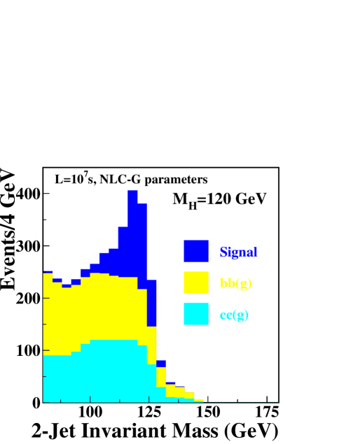
Figure 25: Left: CAIN [127] predictions for the $\gamma\gamma$ luminosity distribution for circularly polarized ($\lambda_{e}=\lambda_{e}^{\prime}=0.4$, $P=P^{\prime}=-1$) and linearly polarized photons assuming $10^{7}$ sec/year, $\sqrt{s}=206{\rm\,GeV}$, 80% electron beam polarization, and a 1.054 micron laser wavelength, after including beamstrahlung and other effects, from [128]. Right: The corresponding value of $\left\langle{\lambda\lambda^{\prime}}\right\rangle$, for circular polarization.

Figure 26: Higgs signal and heavy quark background in $\gamma\gamma\to h$ for a Higgs mass of 120 GeV [128].

In many scenarios, it is possible that by combining this result with other types of precision measurements for the SM-like Higgs boson, small deviations can be observed indicating the possible presence of heavier Higgs bosons. For a 2HDM (either the MSSM or a two-Higgs-doublet model with partial decoupling), if $m_{H^{0}}\sim m_{A^{0}}>\sqrt{s}/2$ then $e^{+}e^{-}\to H^{0}A^{0}$ is not possible and $\gamma\gamma\to H^{0},A^{0}$ may be the only option allowing their discovery (other than implementing higher $\sqrt{s}$). The alternatives of $b\overline{b}H$ and $b\overline{b}A$ production will only allow $H$ and $A$ detection if $\tan\beta$ is large [71]. A LC for which the maximum energy is $\sqrt{s}=630{\rm\,GeV}$ can potentially probe Higgs masses as high as $500{\rm\,GeV}$. If $m_{H^{0}}$ and $m_{A^{0}}$ are known to within roughly $50{\rm\,GeV}$ on the basis of precision $h^{0}$ data, then there is an excellent chance of detecting them by scanning, i.e. stepping in $\sqrt{s}$, using a peaked $\gamma\gamma$ spectrum [57, 128]. If no constraints have been placed on the $H^{0},A^{0}$ masses (other than $m_{A^{0}}\sim m_{H^{0}}>\sqrt{s}/2$), it is best to employ a broad $\gamma\gamma$ spectrum, which would yield a visible signal for $H^{0},A^{0}$ production for only some parameter choices of $m_{A^{0}}$ and $\tan\beta$ [128].

In the non-decoupling 2HDM model with a light decoupled $\widehat{h}$ and all other Higgs bosons heavier than $\sqrt{s}$, $\gamma\gamma\to\widehat{h}\to b\overline{b}$ might allow detection of the $\widehat{h}$ for some of the $\tan\beta$ values in the wedge where the $b\overline{b}\widehat{h}$ and $t\overline{t}\widehat{h}$ production processes both yield fewer than 20 events for an integrated luminosity of 1000 fb^-1 [128].

Once one or several Higgs bosons have been detected, precision studies can be performed including: determination of CP properties; a detailed scan to separate the $H^{0}$ and $A^{0}$ in the decoupling limit of a 2HDM; and branching ratios measurements. The branching ratios to supersymmetric final states are especially important for determining the basic supersymmetry breaking parameters [130, 118, 120, 57].

The CP properties can be determined for any spin-0 Higgs $\widehat{h}$ produced in $\gamma\gamma$ collisions. Since $\gamma\gamma\to{\widehat{h}}$ is of one-loop order, whether ${\widehat{h}}$ is CP-even, CP-odd or a mixture, the CP-even and CP-odd parts of ${\widehat{h}}$ have $\gamma\gamma$ couplings of similar size. However, the structure of the couplings is very different:

$${\cal A}_{{\rm CP}=+}\propto\vec{\epsilon}_{1}\cdot\vec{\epsilon}_{2}\,,\quad{\cal A}_{{\rm CP}=-}\propto(\vec{\epsilon}_{1}\times\vec{\epsilon}_{2})\cdot\widehat{p}_{\rm beam}\,.$$ (17)

By adjusting the orientation of the initial laser photon polarization vectors with respect to one another, it is possible to determine the relative amounts of CP-even and CP-odd content in the resonance ${\widehat{h}}$ [115]. If ${\widehat{h}}$ is a mixture, one can use helicity asymmetries for this purpose [115, 113]. However, if ${\widehat{h}}$ is either purely CP-even or purely CP-odd, then one must employ transverse linear polarizations [116, 113]. Substantial luminosity with transverse polarization can be obtained, although the spectrum is not peaked, as shown in Fig. 26.

One measure of the CP nature of a Higgs is the asymmetry for parallel vs. perpendicular orientation of the linear polarizations of the initial laser beams,

$${\cal A}\equiv{N_{\parallel}-N_{\perp}\over N_{\parallel}+N_{\perp}}\,,$$ (18)

which is positive (negative) for a CP-even (odd) state. Since 100% linear polarization for the laser beams translates into only partial linear polarization for the colliding photons, both $N_{\parallel}$ and $N_{\perp}$ will be non-zero for the signal. In addition, the heavy quark background contributes to both. The expected value of ${\cal A}$ must be carefully computed for a given model. For the SM Higgs with $m_{h_{\rm SM}}=120{\rm\,GeV}$, it is estimated [128] that ${\cal A}$ can be measured with an accuracy of about 20% in one year of operation, assuming the linear polarization spectrum of Fig. 26, 60% linear polarization of the colliding photons, and $S/B$ comparable to that shown in Fig. 26. This measurement would thus provide a moderately strong test of the CP=+ nature of the $h_{\rm SM}$.

We end by noting that the $e^{-}\gamma$ and $e^{-}e^{-}$ collider options are most relevant to exotic Higgs scenarios, as discussed in Section 11.

11 Exotic Higgs sectors and other possibilities

As we have seen, there are many scenarios and models in which the Higgs sector is more complicated than the one-Higgs-doublet of the minimal SM. Supersymmetry requires at least two Higgs doublets. Even in the absence of supersymmetry, a two-doublet Higgs sector allows for CP-violating phenomena. Singlets can also be added without altering the tree-level prediction of $\rho=1$. However, the possibility of Higgs representations with still higher weak (left handed, denoted $L$) isospin should not be ignored. The primary negative is that, for triplets and most higher representations, if the vacuum expectation value of the neutral Higgs field member of the representation is non-zero ($v_{L}\neq 0$) then $\rho$ becomes infinitely renormalized and can no longer be computed [131]; instead it becomes a parameter that must be input as part of the renormalization program. Triplets have received the most attention, as they arise naturally in left-right symmetric extensions of the Standard Model gauge group [132]. (These and other models that utilize Higgs triplets are reviewed in [1].) In this section we will also briefly consider the Higgs-like pseudo-Nambu-Goldstone bosons that arise in generic technicolor theories.

1 A triplet Higgs sector

Including a single complex SU(2)-triplet Higgs representation, in addition to some number of doublets and singlets, results in six additional physical Higgs eigenstates: $H^{--,++}$, $H^{-,+}$, $H^{0}$ and $H^{0\,\prime}$. All but the doubly-charged states can mix with the doublet/singlet Higgs states under some circumstances. Even if $v_{L}\neq 0$ for the neutral field, $\rho=1$ can be preserved at tree-level if, in addition, a real triplet field is also included [133, 134]. However, $\rho$ will still be infinitely renormalized at one-loop unless $v_{L}=0$ is chosen. Left-right symmetric models capable of yielding the see-saw mechanism for neutrino mass generation require two triplet Higgs representations (an L-triplet and an R-triplet). The large see-saw mass entry, $M$, arises from a lepton-number-violating Majorana coupling (which L-R symmetry requires to be present for both the L-triplet and R-triplet representations). Again, $\rho$ will not be altered if $v_{L}=0$, but $v_{R}$ must be non-zero and large for large $M$. We will briefly discuss the phenomenology of an L-triplet. That for the R-triplet of the L-R symmetric model is quite different. (See [1] for a review.)

The resulting Higgs sector phenomenology can be very complex. We focus on the most unequivocal signal for a triplet representation, namely observation of a doubly-charged Higgs boson. Pair production, $Z^{*}\to H^{++}H^{--}$, has limited mass reach, $m_{H^{++}}<\sqrt{s}/2$. Fortunately, single production is also generally possible. Most interestingly, the generically-allowed lepton-number-violating Majorana coupling leads to an $e^{-}e^{-}\to H^{--}$ coupling and the possibility of $s$-channel resonance production of the $H^{--}$ in $e^{-}e^{-}$ collisions. Observation of this process would provide a dramatic confirmation of the presence of the Majorana coupling and, in many cases, the ability to actually measure its magnitude. For a discussion and review, see [135] (and also [136, 137]). If the $H^{--}$ is heavy and has significant $W^{-}W^{-}$ coupling (requiring $v_{L}\neq 0$), then it can become broad and the $s$-channel resonant production cross section is suppressed (see, e.g., [138]) and might not be observable. Another production mechanism sensitive to the $e^{-}e^{-}\to H^{--}$ coupling that might be useful in such an instance is $e^{-}e^{-}\to H^{--}Z$, and $e^{-}e^{-}\to H^{-}W^{-}$ will be sensitive to the $e^{-}\nu_{e}\to H^{-}$ coupling that would be present for the $H^{-}$ member of the triplet representation [139]. Using just the Majorana coupling, doubly-charged Higgs bosons can also be produced via $e^{-}\gamma\to e^{+}H^{--}$ and $e^{+}e^{-}\to e^{+}e^{+}H^{--}$ [140] and the singly-charged members of the same representation can be produced in $e^{-}e^{-}\to H^{-}W^{-}$ [139].

Despite loss of $\rho$ predictivity, it could be that non-zero $v_{L}$ is Nature’s choice. In this case, the $e^{-}e^{-}$ collider option again has some unique advantages. The neutral, singly-charged and doubly-charged Higgs bosons of the triplet representation can all be produced (via $ZZ$ fusion, $W^{-}Z$ fusion and $W^{-}W^{-}$ fusion, respectively). For example, [141] studies $W^{-}W^{-}\to H^{--}$ fusion.

2 Pseudo Nambu Goldstone bosons

In the context of technicolor and related theories, the lowest-mass states are typically a collection of pseudo-Nambu-Goldstone bosons, of which the lightest is very possibly a state $P^{0}$ which can have mass below $200{\rm\,GeV}$ and couplings and other properties not unlike those of a light SM-like Higgs boson. Typically, its $WW,ZZ$ coupling is very small (arising via loops or anomalies), while its $b\overline{b}$ coupling can be larger. The phenomenology of such a $P^{0}$ was studied in [142]. The best modes for detection of the $P^{0}$ at an LC are $e^{+}e^{-}\to\gamma P^{0}\to\gamma b\overline{b}$ and $\gamma\gamma\to P^{0}\to b\overline{b}$. Since the $P^{0}$ is likely to be discovered at the LHC in the $\gamma\gamma$ final state, we will know ahead of time of its existence, and precision measurements of its properties would be a primary goal of the LC.

Chapter 4 Supersymmetry Studies at the Linear Collider

1 Introduction

The Standard Model (SM) has been tested by a spectacularly large and diverse set of experiments. The resulting body of data is consistent with the matter content and gauge interactions of the SM with a Higgs boson of mass $m_{h}\mathrel{\raise 1.29167pt\hbox{$<$\kern-7.5pt\lower 4.30554pt\hbox{$\sim$}}}250~{}{\rm GeV}$ [1]. If a fundamental Higgs boson exists, it fits much more naturally into supersymmetric extensions of the SM than into the SM itself [2, 3, 4, 5]. Thus, the study of supersymmetry (SUSY) is among the highest priorities for future accelerators.

If SUSY exists, many of its most important motivations suggest that at least some superpartners have masses below about $1\,{\rm TeV}$. These motivations, ranging from gauge coupling unification [6, 7, 8, 9, 10] to the existence of an excellent dark matter candidate [11], are discussed in previous chapters and also below. While none of these is a guarantee of SUSY, they all provide motivation for the presence of SUSY at the weak-interaction scale.

In the supersymmetric extension of the SM with minimal field content, hundreds of additional parameters enter the Lagrangian. If SUSY is discovered, this discovery will open new questions—to understand the pattern of the SUSY parameters, to determine from them the mechanism of SUSY breaking, and to infer from them the nature of physics at the very highest energy scales. Such grand goals may be contemplated only if precise and model-independent measurements of superpartner properties are possible.

In this chapter, we describe the prospects for such measurements at a 0.5–1.0 TeV $e^{+}e^{-}$ linear collider (LC) with longitudinally polarized electron beams. The potential of linear colliders for detailed studies of supersymmetry has been discussed previously in numerous reports [12, 13, 14, 15, 16, 17, 18]. In this chapter, many well-established results are reviewed, including the potential for model-independent measurements of superpartner masses. In addition, several less well-appreciated topics are discussed. These include loop-level effects in supersymmetry, CP violation, and supersymmetric flavor violation. This discussion serves both to illustrate the rich program of supersymmetric studies available at linear colliders, and to highlight areas that merit further study. This chapter concludes with a review of the important complementarity of the LC and the Large Hadron Collider (LHC) with respect to supersymmetry studies.

The signatures of supersymmetry are many, ranging from the well-known missing energy in supergravity with R-parity conservation [19, 20] to exotic signatures appearing in models with gauge-mediated [21] and anomaly-mediated [22, 23] supersymmetry breaking. Space constraints prevent a complete review of the considerable work done in each of these, and other, frameworks. Instead, this review focuses on supergravity frameworks leading to the conventional signature of missing energy. R-parity violation and alternative supersymmetry-breaking mechanisms are treated as variations, and are discussed where they are especially pertinent.

2 The scale of supersymmetry

The cleanliness of the linear collider environment implies that precise, model-independent measurements in supersymmetry are possible, but only if supersymmetric final states are kinematically accessible. The mass scale of supersymmetric particles is therefore of paramount importance. In this section we review bounds on superpartner masses from naturalness criteria, dark matter constraints, Higgs boson searches, and precision electroweak data. We also consider the potential of experimental evidence for new physics to constrain the supersymmetric mass scale; we discuss the muon anomalous magnetic moment as an example.

1 Naturalness

In supersymmetric extensions of the SM, quadratically divergent quantum corrections to the masses of fundamental scalars are of the order of the superpartner mass scale. Given a mechanism for producing sufficiently light superpartners, the observed weak scale is obtained without unnaturally large cancellations in the electroweak potential. While no analysis of naturalness can claim quantitative rigor, the importance of naturalness as a fundamental motivation for supersymmetry has prompted many studies [24, 25, 26, 27, 28, 29, 30, 31, 32, 33, 34, 35, 36, 37, 38, 39, 40, 41, 42, 43, 44, 45, 46], with important qualitative implications for the superparticle spectrum.

To study naturalness one must first assume a certain supersymmetric framework. Models in this framework are specified by a set of input parameters, typically defined at some high energy scale. Together with experimental constraints and renormalization group equations, these parameters determine the entire weak-scale Langrangian, including the $Z$ boson mass, which at tree level is

$$\frac{1}{2}m_{Z}^{2}=\frac{m_{H_{d}}^{2}-m_{H_{u}}^{2}\tan^{2}\beta}{\tan^{2}\beta-1}-\mu^{2}\ ,$$ (1)

where $m_{H_{d}}^{2}$, $m_{H_{u}}^{2}$ are the mass parameters of the two Higgs doublets of the model and $\tan\beta=\left\langle{H_{u}}\right\rangle/\left\langle{H_{d}}\right\rangle$. Naturalness is then often imposed by demanding that the weak scale be insensitive to variations in some set of parameters $a_{i}$, which are assumed to be continuously variable, independent, and fundamental. The $a_{i}$ may be scalar masses, gaugino masses, and other parameters, but are not necessarily input parameters. The sensitivity is typically quantified by defining coefficients [24, 25] $c_{i}\equiv\left|(a_{i}/m_{Z})(\partial m_{Z}/\partial a_{i})\right|$ for each parameter $a_{i}$ and taking some simple combination of the $c_{i}$, often $c=\max\{c_{i}\}$, as an overall measure of naturalness. A naturalness criterion $c<c_{\rm max}$ then implies upper bounds on supersymmetry parameters and superpartner masses.

Following the early studies [24, 25], the authors of [27] stressed the importance of including one-loop corrections to Eq. (1). They also noted that it is possible in principle for a given $c_{i}$ to be large for all possible choices of $a_{i}$. In the latter case, the authors of [28, 29, 30] argued that, to avoid misleading results, only unusually large sensitivity should be considered unnatural and proposed replacing $c$ by $\tilde{\gamma}\equiv\max\{c_{i}/\overline{c}_{i}\}$, with $\overline{c}_{i}$ an average sensitivity. More recently, another alternative prescription has been proposed [34, 35, 36, 37, 38] in which the sensitivity coefficients are replaced by $\left|(\Delta a_{i}/m_{Z})(\partial m_{Z}/\partial a_{i})\right|$, where $\Delta a_{i}$ is the experimentally allowed range of $a_{i}$. This definition implies that arbitrarily large but well-measured supersymmetry parameters are natural, and has been argued to differ sharply from conventional notions of naturalness [46].

The results of naturalness studies are strongly dependent on the choice of framework, the choice of fundamental parameters $a_{i}$, and, of course, the choice of $c_{\rm max}$ (or the equivalent $\tilde{\gamma}$ parameter). The dependence on framework assumptions is inescapable. In other studies of supersymmetry there exists, at least in principle, the possibility of a model-independent study, where no correlations among parameters are assumed. In studies of naturalness, however, the correlations determine the results, and there is no possibility, even in principle, of an all-inclusive framework. We describe here only some of the qualitatively distinct possibilities. For alternative analyses, readers are referred to the original literature [24, 25, 26, 27, 28, 29, 30, 31, 32, 33, 34, 35, 36, 37, 38, 39, 40, 41, 42, 43, 44, 45, 46].

In minimal supergravity, one assumes both scalar and gaugino universality at a high scale. If one requires insensitivity of the weak scale with respect to both supersymmetry breaking and Standard Model parameters, none of the superpartner masses can naturally be far above the weak scale. Examples of the resulting naturalness bounds are given in Fig. 1. The bounds for non-strongly interacting superpartners are typically more stringent than those for colored superpartners. Similar results are found in other frameworks where all scalar and gaugino masses are comparable at some high scale.

Figure 1: Natural ranges of superpartner masses in minimal supergravity. The upper limits are set by the requirement $\tilde{\gamma}<10$ and the diamonds indicate upper bounds corresponding to $\tilde{\gamma}<5$. The lower limits are roughly those from current collider constraints. Updated from [29].

Naturalness bounds may be very different in other frameworks, however, especially for scalars. For squark and slepton masses, if no correlations are assumed, the bounds are highly generation-dependent. At one-loop, the weak scale is sensitive to sfermion masses only through renormalization group terms proportional to Yukawa couplings. Thus, while the scalar masses of the third generation are still usefully constrained by naturalness criteria, first- and second-generation scalars may have masses above $10~{}{\rm\,TeV}$ without requiring large fine-tuning [31, 32], putting them far beyond the kinematic reaches of both the LHC and future linear colliders. ‘Superheavy’ first and second generation scalars ameliorate the supersymmetric flavor and CP problems and are found in many models [47, 48, 49, 50, 51, 52, 53, 54, 55, 56, 57, 58, 59, 60, 61, 62, 63].

Alternatively, given the possibility that SM couplings are fixed in sectors separate from supersymmetry breaking, one may reasonably require only that the weak scale be insensitive to variations in parameters related to supersymmetry breaking [44, 45, 46]. With this less stringent criterion, in many simple models, including minimal supergravity, all scalar partners may be naturally in the 2–3 TeV range, as a result of focusing behavior in renormalization group trajectories [44, 45, 46, 64, 65, 66, 67, 68]. Such “focus point supersymmetry” models also have significant virtues with respect to low-energy constraints, and predict that even third-generation scalars may have masses well above 1 TeV and be beyond the reach of linear colliders.

Bounds on the masses of fermionic superpartners are less framework-dependent. If the gaugino masses are uncorrelated, the gluino mass is typically stringently bounded by its indirect influence on the weak scale through the top squarks. In this general context, the electroweak gaugino masses may be significantly larger [42, 43]. However, in most well-motivated models, the gluino is much heavier than the electroweak gauginos, and so naturalness implies stringent limits on Bino and Wino masses. While the scale of the $\mu$ parameter may be determined [69], a quantitative theory for the $\mu$ term is lacking. The $\mu$ parameter is therefore usually determined through Eq. (1) and is otherwise assumed to be uncorrelated with other parameters. Large $\mu$ then necessarily leads to large fine-tuning, and so heavy Higgsinos are disfavored. As a result, given our present understanding, naturalness criteria typically imply relatively stringent bounds on the masses of all six chargino and neutralino states, and they encourage the expectation that all of these particles will be available for study at linear colliders.

2 Neutralino relic abundance

An important virtue of many supersymmetric theories is the existence of a non-baryonic dark matter candidate. The most straightforward possibility is the lightest neutralino $\chi$ [11, 70], which is often the lightest supersymmetric particle (LSP) and so is stable in models with conserved R-parity. Current cosmological and astrophysical measurements prefer $0.1\mathrel{\raise 1.29167pt\hbox{$<$\kern-7.5pt\lower 4.30554pt\hbox{$\sim$}}}\Omega_{m}h^{2}\mathrel{\raise 1.29167pt\hbox{$<$\kern-7.5pt\lower 4.30554pt\hbox{$\sim$}}}0.3$ [71], where $\Omega_{m}$ is the ratio of dark matter density to critical density, and $h\approx 0.65$ is the Hubble parameter in units of $100\,{\rm km\,s^{-1}\,Mpc^{-1}}$. The superpartner spectrum is then constrained by the requirement that the thermal relic density of the lightest neutralino satisfy $\Omega_{\chi}h^{2}\mathrel{\raise 1.29167pt\hbox{$<$\kern-7.5pt\lower 4.30554pt\hbox{$\sim$}}}0.3$.

The neutralino relic density is determined by the neutralino pair annihilation cross section and has been the subject of many analyses [72, 73, 74, 75, 76, 77, 78, 79, 80, 81, 82, 83, 84, 85, 86, 87, 88, 89, 90, 91, 92, 93, 94, 95, 96, 97, 98, 99, 100]. These include refined treatments of poles [72, 73, 74], annihilation thresholds [72, 73], and co-annihilation among Higgsinos [75] and with staus [76, 77]. The S- and P-wave contributions to all tree-level processes with two-body final states are given in [78].

In general, neutralinos may annihilate through $t$-channel sfermions to $f\overline{f}$ , through $s$-channel $Z$ and Higgs bosons to $f\overline{f}$, and through $t$-channel charginos and neutralinos to $WW$ and $ZZ$. For Bino dark matter, only the sfermion-mediated amplitudes are non-vanishing. An upper bound on $\Omega_{\chi}h^{2}$ then leads to an upper bound on at least one sfermion mass. This, together with the requirement that $\chi$ be the LSP, implies an upper bound on $m_{\chi}$. Such reasoning has led to claims of cosmological upper bounds on superpartner masses with optimistic implications for supersymmetry at linear colliders [79, 80, 81, 82, 83, 84, 85, 86, 87, 88, 89].

These claims must be viewed cautiously, however, as they are true only in the $\chi\approx\tilde{B}$ limit and are violated even in the simplest scenarios. In minimal supergravity, for example, multi-TeV LSPs are possible for large $m_{0}$ [94], where the LSP has a significant Higgsino admixture, leading to large annihilation cross sections to gauge bosons. Useful upper bounds are also absent in minimal supergravity at large $\tan\beta$ [94, 95, 96, 97], where the importance of a small Higgsino admixture in $\chi$ is amplified and leads to large Higgs boson-mediated annihilation. More generally, no guarantee of light superpartners is possible for Wino- [98, 99, 100] and Higgsino-like [75, 90] LSPs, which annihilate very efficiently to negligible relic densities. Finally, it is worth recalling that these upper bounds are also inapplicable in theories with low-energy supersymmetry breaking or R-parity violation, where the lightest neutralino is no longer stable.

3 Higgs mass and precision electroweak constraints

As is well known, supersymmetry places severe constraints on the mass of the lightest Higgs boson. In the Minimal Supersymmetric Standard Model (MSSM), one-loop calculations [101, 102, 103, 104, 105, 106, 107, 108, 109, 110] have now been supplemented with leading two-loop corrections in the Feynman diagrammatic [111, 112, 113, 114, 115], renormalization group [116, 117, 118, 119], and effective potential [120, 121, 122] approaches, leading to an upper bound of $m_{h}\mathrel{\raise 1.29167pt\hbox{$<$\kern-7.5pt\lower 4.30554pt\hbox{$\sim$}}}135~{}{\rm\,GeV}$ [113]. The consistency of this bound with precision electroweak fits is a considerable success of supersymmetry. At the same time, though, one might expect that the current lower bound $m_{h}>113.5~{}{\rm\,GeV}$ from direct Higgs searches [123, 124, 125, 126] and the success of precision electroweak fits to the SM disfavors the possibility of light superpartners.

However, closer analysis shows that light superpartners are consistent with the current Higgs mass bound. For example, in general scenarios, the current Higgs mass limit may be satisfied with large masses only for the top and bottom squarks. Even for these, the constraints are not severe. Charginos, neutralinos, and sleptons may be light and within the reach of linear colliders. In simpler frameworks, the Higgs limit is more constraining. Even in minimal supergravity, however, the current Higgs mass bound, along with the requirement of a suitable dark matter candidate, may be satisfied either for chargino masses above 200 GeV [127] or for large $m_{0}$ [46, 128]. In the latter case, charginos may be as light as their current LEP bound. The Higgs mass bound can also be made consistent with light superpartners if there are large CP-violating phases, which must necessarily cancel to high accuracy in electric dipole moments, or new singlets [129]. Thus, the current Higgs mass constraint, although already rather stringent, does not exclude the possibility of light superpartners.

The supersymmetric spectrum is also constrained by precision electroweak measurements. The effects of supersymmetry have been studied in numerous recent works (see, e.g., [130, 131, 132, 133, 134, 135]). While there are at present no strong indications for supersymmetry from these considerations, light superparticles cannot be excluded either. This issue is discussed further in Chapter 8, Section 3.2.

4 Evidence for new physics

Finally, weak-scale supersymmetry has implications for a broad range of experiments in particle physics and astrophysics. If deviations from SM predictions are found, these deviations may also constrain the scale of superpartner masses.

As an example, we consider the recently reported 2.6$\sigma$ deviation in the anomalous magnetic moment of the muon [136]: $a_{\mu}^{\rm exp}-a_{\mu}^{\rm SM}=(43\pm 16)\times 10^{-10}$. Supersymmetric contributions to $a_{\mu}$ are well known [137, 138, 139, 140, 141], and the measured deviation is naturally explained by supersymmetry [142, 143, 144, 145, 146, 147, 148, 149, 150, 151, 152, 153]. If a supersymmetric interpretation is adopted, the result restricts the masses of some superpartners. Highly model-independent upper bounds on the mass of the lightest observable supersymmetric particle are given in Fig. 2. If theory and experiment are required to agree within 1$\sigma$, at least one observable superpartner must be lighter than 490 GeV if the LSP is stable, and lighter than 410 GeV if the LSP decays visibly in the detector. If agreement only within 2$\sigma$ is required, these limits weaken to 800 GeV and 640 GeV, respectively. The bounds are for the case $\tan\beta\leq 50$ and scale linearly with $\tan\beta$.

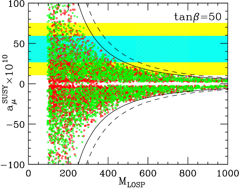
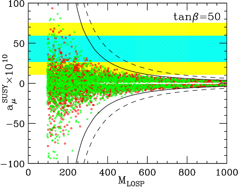
Figure 2: Possible values of the mass of the lightest observable supersymmetric particle, $M_{\rm LOSP}$, and the supersymmetric contribution to the muon’s anomalous magnetic moment, $a_{\mu}^{\rm SUSY}$, assuming a stable LSP (left) and a visibly decaying LSP (right). Crosses (circles) have smuon (chargino/neutralino) LOSPs and satisfy the parameter constraints $M_{2}=2M_{1}$, $A_{\mu}=0$, and $\tan\beta=50$. Relaxing the gaugino unification assumption leads to the solid envelope curve, and further allowing arbitrary $A_{\mu}$ leads to the dashed curve. The envelope contours scale linearly with $\tan\beta$. The shaded regions are the 1$\sigma$ and 2$\sigma$ experimentally preferred regions. From [144].

These results illustrate the power of evidence for new physics to constrain the scale of supersymmetry. Of course, many other experiments may also see supersymmetric effects. Among the areas in which great experimental progress is expected in the next few years are searches for new physics at the Tevatron, $B$ physics (CP violation, rare decays), lepton flavor violation ($\mu$-$e$ conversion, $\mu\to e\gamma$, etc.), electric dipole moments, searches for dark matter (both direct and indirect), and cosmic ray physics. Pre-LHC evidence for supersymmetry is not guaranteed, but, in simple frameworks like minimal supergravity where systematic and comprehensive analyses are possible, it is very likely [95]. Strong evidence for new physics, even if indirect, will provide important additional constraints on the mass scale of supersymmetric particles.

3 Determination of masses and couplings

The usefulness of a linear collider in the study of SUSY particles lies both in the simplicity of the production process and in the fact that the electron can have a large longitudinal polarization. These features allow one to carry out accurate measurements of the masses and the quantum numbers of the particles being produced, and also to determine their gauge coupling constants in a model-independent manner [154, 155]. Such measurements are crucial in understanding the nature of the processes being uncovered.

1 Measurement of superpartner masses

We begin our review of mass measurements by considering one particular process that illustrates the essential simplicity of the analyses. The process we will consider is selectron production,

$$e^{+}e^{-}\to\widetilde{e}_{L,R}^{+}\widetilde{e}_{L,R}^{-}\ ,$$ (2)

where $\widetilde{e}_{R}^{-}$, $\widetilde{e}_{L}^{-}$ are the supersymmetry partners of the right- and left-handed electron. We assume that both selectrons decay by $\widetilde{e}_{L,R}\rightarrow e\widetilde{\chi}_{1}^{0}$. The process has a number of interesting features. The masses of the $\widetilde{e}_{R}$ and $\widetilde{e}_{L}$ can differ substantially. The combinations $\widetilde{e}_{R}^{+}\widetilde{e}_{R}^{-}$ and $\widetilde{e}_{L}^{+}\widetilde{e}_{L}^{-}$ are produced by $s$-channel photon and $Z^{0}$ exchange, but all four possible selectron combinations are produced by $t$-channel neutralino exchange. Thus, the study of this process can give information on SUSY masses, quantum numbers, and coupling constants.

In the reaction (2), the selectrons are produced at a fixed energy. Since they are scalars, they decay isotropically in their own frames. These distributions of the decay electrons and positrons boost to distributions in the lab that are flat in energy between the kinematic endpoints. The electrons and positrons then show box-like distributions. The maximum and minimum energies which form the edges of the box determine the masses of the $\widetilde{e}$ and the $\widetilde{\chi}_{1}^{0}$ through the relations

$$M_{\widetilde{e}}^{2} = {E_{\rm cm}^{2}}\left\{{{E_{e,\rm max}E_{e,\rm min}}\over{(E_{e,\rm max}+E_{e,\rm min})^{2}}}\right\}$$

$$M_{\widetilde{\chi}_{1}^{0}}^{2} = M_{\widetilde{e}}^{2}\left\{1-2{{E_{e,\rm max}+E_{e,\rm min}}\over{E_{\rm cm}}}\right\}\ .$$

If several different combinations of selectrons are produced, the electron and positron energy spectra will show a superposition of several box-like distributions. Each set of endpoints gives the associated selectron masses and an independent determination of the $\widetilde{\chi}_{1}^{0}$ mass.

Figure 3 shows the electron and positron spectra for a particular set of MSUGRA parameters constructed for the Snowmass ‘96 summer study [156], assuming 50 fb^-1 of data at $\sqrt{s}=500$ GeV [157]. The simulations use the event generator ISAJET [158]. The expected box-like spectra appear clearly, with sharp endpoints. Both the electron and positron spectra have a strong dependence on polarization, and this allows us to recognize which components are associated with $\widetilde{e}_{L}$ and which with $\widetilde{e}_{R}$. The electron and positron spectra also differ from each other, reflecting the different production of $\widetilde{e}_{R}^{-}\widetilde{e}_{L}^{+}$ versus $\widetilde{e}_{L}^{-}\widetilde{e}_{R}^{+}$ from polarized beams.

Figure 4  compares the generated electron and positron distributions to those reconstructed using energy measurements from the electromagnetic calorimeter of the L detector described in Chapter 15. The study uses full GEANT simulation of the calorimeter [159]. The effect of resolution is clearly observed in the upper edge of the energy distribution. This analysis does not include beamstrahlung and initial state radiation, but these effects are not expected to affect significantly the determination of the edges in the energy spectra [156].

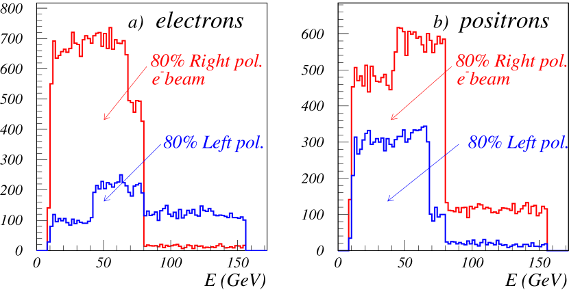
Figure 3: Electron and positron energy distributions for selectron pair production, with the indicated beam polarizations and integrated luminosity 50 fb^-1 [157].

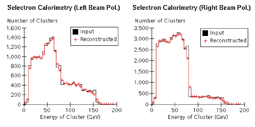
Figure 4: Input and calorimeter-reconstructed $e^{\pm}$ energy distributions from selectron pair production for 80% left-polarized (left) and 80% right-polarized (right) electron beams [159]. The effect of calorimeter resolution is evident at high cluster energies.

Reference	Particle	Input	Measured	Particle	Input	Measured
[157]	$\widetilde{e}_{L}^{\pm}$	238.2	239.4	$\widetilde{\chi}_{1}^{0}$	128.7	129.0
[157]	$\widetilde{e}_{R}^{\pm}$	157.0	158.0	$\widetilde{\chi}_{1}^{0}$	128.7	129.0
[173]	$\widetilde{\mu}_{R}^{\pm}$	157.1	143.2	$\widetilde{\chi}_{1}^{0}$	128.7	117.3
[162]	$\widetilde{\nu}_{e}$	206.6	199.4	$\widetilde{\chi}_{1}^{\pm}$	96.4	96.5
[154]	$\widetilde{\chi}_{1}^{\pm}$	219.0	212.0	$\widetilde{\chi}_{1}^{0}$	118.0	116.5
[165]	$\widetilde{\chi}_{1}^{\pm}$	238.0	239.8	$\overline{\widetilde{\nu}}_{\ell}$	220.0	221.2
[163]	$\widetilde{\chi}_{2}^{\pm}$	175.2	176.5	$\widetilde{\chi}_{1}^{\pm}$	85.9	86.1
[166]	$\widetilde{\chi}_{2}^{\pm}$	290.4	282.7	$\widetilde{\chi}_{1}^{\pm}$	96.0	97.9

Table 1: Comparison of the input and measured masses (in GeV) for a few supersymmetric particles as determined from the end-point spectrum of the observed particles smeared via fast MC techniques. Most of the results are based on a 50 fb^-1 data sample. The pair of masses in each row are determined from the end-point measurement in pair-production of the first particle listed.

Many similar analyses of the determination of slepton masses have been carried out using fast Monte Carlo techniques [160, 161, 162, 163]. Some of the results are summarized in Table 1. One can see from the table that we expect to be able to measure these masses with an accuracy of a few percent or less in most cases. The determination of the mass of the lighter chargino $\widetilde{\chi}_{1}^{\pm}$ has been studied by many groups. Measurements based on an analysis using background cuts [154, 163, 164] indicate that this mass can be measured with accuracies of 1% or less by this method. An interesting signal thast may be background-free is the case where one $\widetilde{\chi}_{1}^{\pm}$ decays into a lepton and a $\overline{\widetilde{\nu}}_{\ell}$, with the $\overline{\widetilde{\nu}}_{\ell}$ decaying to a $\nu\widetilde{\chi}_{1}^{0}$, while the other $\widetilde{\chi}_{1}^{\pm}$ decays into $q\overline{q}\widetilde{\chi}_{1}^{0}$. In this case, it should be possible to remove the $WW$ background completely without affecting the signal [165]. The mass measurement for the heavier chargino $\widetilde{\chi}_{2}^{\pm}$ has also been studied, assuming a CM energy of 750 GeV. By using the decay of the $\widetilde{\chi}_{2}^{\pm}$ into $\widetilde{\chi}_{1}^{\pm}Z^{0}$, where the $Z$ decays into leptons and the $\widetilde{\chi}_{1}^{\pm}$ decays into hadrons, one is able to get quite accurate results [166]. The conclusions of all these analyses are also shown in Table 1.

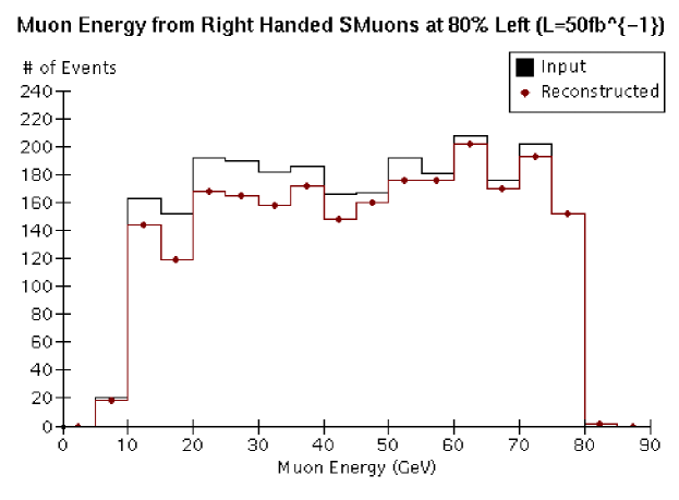
Figure 5: Input and tracker-reconstructed muon energy spectra from smuon pair production with an 80% left-polarized electron beam [173].

It is worth reviewing some of the experimental issues that arise in these measurements. We have already given an example in which the calorimeter resolution affects the mass measurements for selectrons decaying to $e^{-}$ and $e^{+}$. For the case of smuons decaying to $\mu^{\pm}$, the corresponding issue is tracking resolution. In Fig.  5, we show a comparison of generator-level and reconstructed muon energy in $\widetilde{\mu}$ pair production. It is clear that the tracking reconstruction does not significantly affect the energy edge resolution, and hence it does not affect our ability to determine supersymmetric masses accurately. For chargino decays, both calorimeter and tracking resolution enter the determination of kinematic endpoints [154].

To examine the supersymmetry signals, it is necessary to remove backgrounds events efficiently. The major sources of SM backgrounds are the two-photon ($\gamma^{\star}\gamma^{\star}$) process, which gives rise to lepton and quark pairs in the detector, $e^{+}e^{-}$ annihilation to the $W^{+}W^{-}$, $Z^{0}Z^{0}$, and $Z^{0}h^{0}$, and single-$W$ production ($e\gamma^{*}\to\nu W$). Methods for removing the annihilation and single $W$ backgrounds from the supersymmetry sample are explained in [154, 167, 168]. The two-photon background is a problem in reactions whose signatures involve missing energy, but it can be controlled by also requiring missing transverse momentum. Methods for measuring the two-photon background have been studied in [169, 168, 170, 171, 172]. There may also be backgrounds from the decays of other supersymmetric particles but, in most cases, these are either small or have distinctive signals that allow one to identify them.

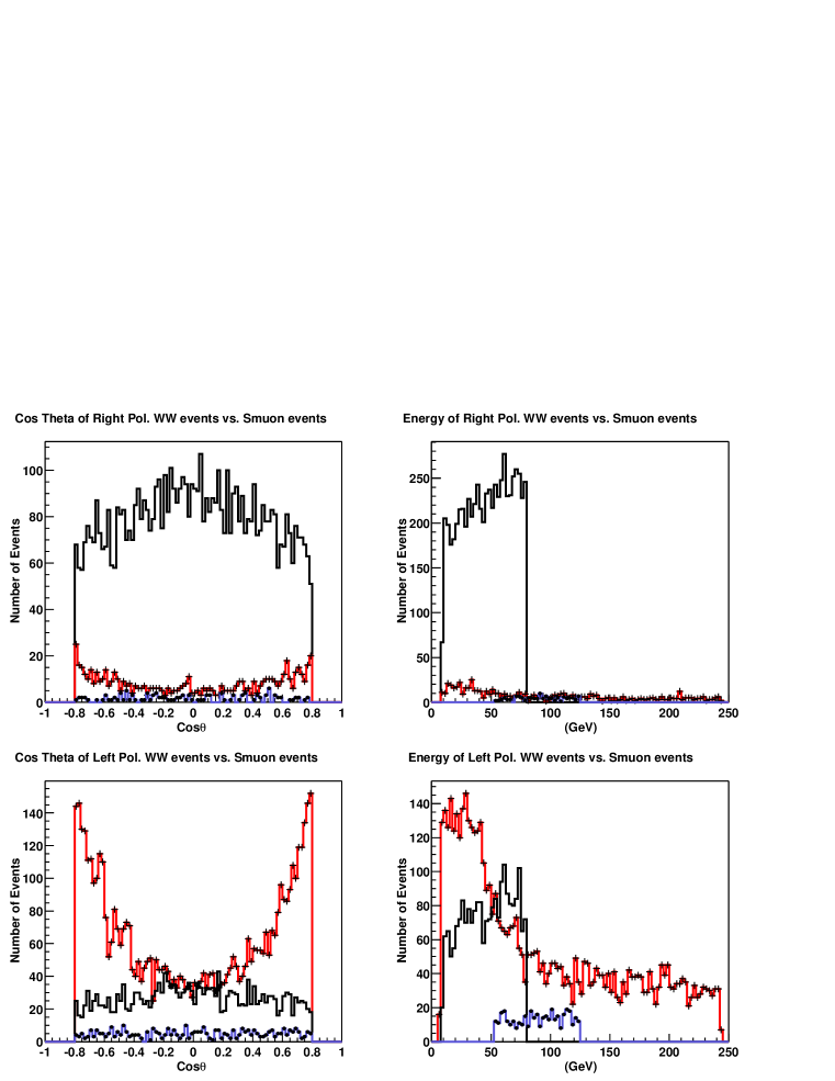
Figure 6: Kinematic distributions of muons from $\widetilde{\mu}_{R}$ pair production (solid), $\widetilde{\mu}_{L}$ pair production (dotted), and $W^{+}W^{-}$ background (crossed) [173]. An electron beam polarization of 80% is assumed.

One case in which $W$ pair production is a serious background is the study of the muon energy spectrum $\widetilde{\mu}_{R,L}^{\pm}$. The cross section for $\widetilde{\mu}$ pair production is small, and the $W$ pair production process leads to muon pairs with missing transverse momentum from neutrinos. Figure 6 shows the effect of the $W$ pair background after appropriate cuts  [173]. The figure also shows that electron polarization can be used to remove this background. The $\widetilde{\mu}_{R}$ signal is most clearly seen with a right-handed polarized electron beam, since the $W^{+}W^{-}$ production is strongly reduced in this case. Observing the signal for $\widetilde{\mu}_{L}$ is difficult with either polarization. If the model parameters are such that the $\widetilde{\ell}_{R,L}$ is heavier than the $\widetilde{\chi}_{2}^{0}$, this problem can be avoided by studying the decay $\widetilde{\ell}_{R,L}^{\pm}$$\rightarrow\ell^{\pm}+\widetilde{\chi}_{2}^{0}$, with the $\widetilde{\chi}_{2}^{0}$ decaying to a lepton pair and $\widetilde{\chi}_{1}^{0}$. Then, because of the large lepton multiplicity, there are no important SM backgrounds [174].

Another kinematic method for determining the masses of supersymmetric particles is to exploit the correlations between the products of the two decaying sparticles in a given event [175]. This technique is especially useful in cases where low-$p_{T}$ backgrounds tend to overwhelm the signal. Some experimental analyses have been carried out using this method [176, 177], and it should receive more attention.

One can also carry out mass measurements using threshold scans [174, 164], though in some cases this requires 100 fb^-1 of luminosity per threshold. The method has the potential to measure masses with accuracies of 0.1%. The effect of backgrounds from SM processes and other SUSY signals and the effects of beamstrahlung and bremsstrahlung need to be understood to determine the systematics limits of this method [178].

A special case of spectrum parameters for which SUSY detection and mass measurement are especially difficult is that of an almost-degenerate chargino and neutralino. This situation can occur in the Higgsino limit of gaugino-Higgsino mixing, and in anomaly-mediated supersymmetry breaking (AMSB). A recent analysis [179] shows how to extract the chargino signal in this limit using the reaction e⁺e${}^{-}\rightarrow\gamma\widetilde{\chi}_{1}^{+}\widetilde{\chi}_{1}^{-}$. In some cases, in particular, those from AMSB, the $\widetilde{\chi}_{1}^{\pm}$ has a long enough lifetime that, at the linear collider, one can see the chargino’s track in the vertex detector before it decays. One then observes a stiff track turning into a very soft track, which would be a dramatic signal.

Table 1 makes clear that it is possible to measure the first-generation slepton masses with a precision of about 1%. This would allow experiments at linear colliders to probe the underlying GUT-scale universality of intra-generation slepton masses, with enough sensitivity to discriminate the MSUGRA framework from other models (e.g., gaugino-mediation) where small GUT-scale splittings of sleptons are expected [180]. Another important observation from Table 1 is that the linear collider measurements of SUSY particles will provide multiple high-accuracy measurements of the mass of the lightest neutralino $\widetilde{\chi}_{1}^{0}$. As we will discuss in Section 7, this information will directly complement supersymmetry measurements at the LHC, since this key parameter will not be well determined there.

2 Measurement of supersymmetry parameters

Once superpartners are identified and their masses are measured, it is important to convert the mass and cross section information into determinations of the parameters of the SUSY theory. For the example of the MSSM with R-parity conservation, studies have been done to determine how well one can measure the fundamental parameters. By studying the production and subsequent decays of $\widetilde{\chi}_{1}^{\pm}$ and $\widetilde{\chi}_{2}^{\pm}$, the masses and the gaugino-higgsino mixing angles of these states can be measured and hence the values of the MSSM parameters $M_{2}$, $\mu$, and tan$\beta$ can be determined to about 1% accuracy [155, 181, 182]. This is illustrated in Fig. 7, where it is shown that the value of the chargino production cross section from a right-handed polarized beam allows one to map out whether the lighter chargino is mainly gaugino or Higgsino. A measurement of both the cross section and the angular distribution allows one to measure all of the terms in the chargino mass matrix. It should be noted that the figure shows the tree-level cross section. A true determination of parameters to 1% accuracy should take account of electroweak and SUSY radiative corrections.

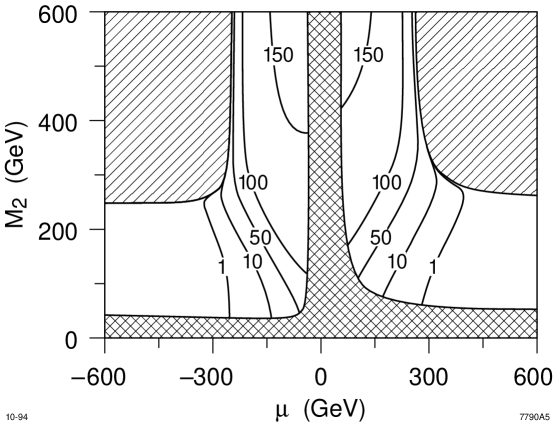
Figure 7: The dependence of the chargino production cross section $\sigma(e_{R}^{-}e^{+}\to\widetilde{\chi}^{+}_{1}\widetilde{\chi}^{-}_{1})$, in fb, on M₂ and $\mu$ [155]. The value $\tan\beta=4$ is used for this plot, but the result is only weakly dependent on this parameter.

Another method for determining whether the lightest neutralinos and chargino are mostly gaugino or Higgsino is to study slepton pair production with left-handed and right-handed beam polarization. This is done by measuring the magnitude of the cross section and the shape of the production angular distribution [154]. Similarly, measuring the cross sections of $\widetilde{t}_{1}$, $\widetilde{t}_{2}$, $\widetilde{\tau}_{1}^{\pm}$ and $\widetilde{\tau}_{2}^{\pm}$ and $\overline{\nu}_{\tau}$ with polarized beams allows one to determine their mixing angles [183, 184, 185]. Additional measurements associated with polarization in $\widetilde{\tau}$ reactions are discussed in [154, 186].

By looking at the angular distributions of supersymmetric particles that have a $t$-channel exchange involving another supersymmetric particle, the mass of the exchanged particle can be determined. Similarly, if the decays of the charginos have three-body decays because the two-body decay to $W\widetilde{\chi}^{0}_{1}$ is not allowed kinematically, decays via $W^{*}$ can interfere with decays involving a virtual slepton or squark. This could give useful indirect signals for these particles in the cases where they cannot be produced because they are too heavy [187].

We should recall that the parameter $\tan\beta$ can be determined not only from supersymmetry reactions but also by direct experimental studies of the extended Higgs sector. For $\tan\beta<30$, one can obtain an accurate value of this parameter by measuring the branching ratios for the various possible decays of the SUSY Higgs particles: $H^{-}$ into $\tau\nu$, $b\overline{t}$, and $W^{-}h$, and $A^{0}$ and $H^{0}$ into $\tau^{+}\tau^{-}$, $b\overline{b}$, $t\overline{t}$, and $Zh$ [188, 189]. If the Higgs sector is heavy enough, one can include decays into lighter supersymmetric particles. These can provide quite sensitive measurements in the high-tan$\beta$ region [189].

Finally, it is important to verify the spin of each supersymmetric partner experimentally. This can be done at a linear collider, because the simplicity of the production reactions often makes the spin obvious from the angular distributions. For example, the $\widetilde{\mu}_{R}$ signal in Fig. 6 exhibits a $\sin^{2}\theta$ distribution that is a clear indication that the spin of the $\widetilde{\mu}_{R}$ is 0. The spin of supersymmetric particles can also be determined by measuring the pair-production cross section near threshold, which rises as $\beta$ and $\beta^{3}$, where $\beta$ is the particle velocity, for spin-$\frac{1}{2}$ and spin-0 particles, respectively.

4 Tests of supersymmetry

If new particles are discovered with quantum numbers expected in supersymmetry, it is desirable to determine whether they are in fact superparticles. Linear colliders can verify supersymmetry through highly model-indepedent tests accurate at the percent level. In addition, since these tests are sensitive to loop-level effects, they may yield a wealth of additional information.

Supersymmetry may be tested in many ways. For example, confirmation that some of the newly discovered particles are scalars, as discussed at the end of Section 3, constitutes an important, if weak, test of supersymmetry. More quantitatively, verification of the consistency of direct discoveries with the expected indirect supersymmetric effects in SM processes, as discussed in Chapter 8, Section 3, also provides a test of supersymmetric interpretations of new physics. Measurements of the mass differences between scalar partners in the same SU(2) doublet may also provide quantitative and rather model-independent checks.

In this section we focus on investigations of supersymmetric coupling relations, which are among the most incisive and model-independent tests. In addition to providing precise quantitative confirmation of supersymmetry, such tests may also shed light on otherwise inaccessible superpartners, much as current precision electroweak measurements bound the Higgs boson mass and constrain new physics.

1 Confirming supersymmetry

If supersymmetry were an exact symmetry of nature, the properties of supersymmetric particles would be completely determined by the properties of their SM partners. Of course, relations between masses are broken by soft supersymmetry breaking parameters. However, supersymmetry also predicts the equivalence of dimensionless couplings. For example, supersymmetry implies

$$g_{i}=h_{i}\ ,$$ (3)

where $g_{i}$ are the SM gauge couplings, $h_{i}$ are their supersymmetric analogues, the gaugino-fermion-sfermion couplings, and the subscript $i=1,2,3$ refers to the U(1), SU(2), and SU(3) gauge groups, respectively. These identities are not broken by soft supersymmetry-breaking parameters at tree level and are therefore known as “hard supersymmetry relations” [190]. They are valid in all supersymmetric theories, in contrast to other predictions such as the universality of scalar or gaugino masses. Hard supersymmetry relations therefore provide, in principle, a model-independent method of quantitatively confirming that newly-discovered particles are indeed superpartners [155, 183].

2 Super-oblique corrections

At the loop-level, however, even hard supersymmetry relations receive corrections that would vanish in the supersymmetric limit [191]. These corrections are analogous to the oblique corrections [192] of the Standard Model. In the SM, SU(2) multiplets with custodial SU(2)-breaking masses, such as the $(t,b)$ multiplet, induce splittings in the couplings of the $(W,Z)$ vector multiplet at the quantum level. Similarly, in supersymmetric models, supermultiplets with soft supersymmetry-breaking masses, such as the $(\tilde{f},f)$ supermultiplets, induce splittings in the couplings of the $({\rm gauge\ boson},{\rm gaugino})$ vector supermultiplet at the quantum level. This analogy can be made very precise [193, 194, 195, 196]. Corrections to hard supersymmetry relations are therefore called ‘super-oblique corrections’, and the splittings are typically written in terms of ‘super-oblique parameters.’

If some scalar superpartners $\tilde{f}$ have masses at a high scale $M$, and all others are light with mass $m\sim M_{\rm weak}$, the super-oblique parameters are given by

$$\widetilde{U}_{i}\equiv\frac{h_{i}(m)}{g_{i}(m)}-1\approx\frac{g_{i}^{2}(m)}{16\pi^{2}}\Delta b_{i}\ln\frac{M}{m}\ ,$$ (4)

where $\Delta b_{i}$ is the one-loop $\beta$-function coefficient contribution from all light particles whose superpartners are heavy. Equation (4) is the leading logarithm contribution to $\widetilde{U}_{i}$. The super-oblique parameters for some representative models are given in Table 2. The super-oblique parameters may also receive contributions from split exotic supermultiplets, such as the messengers of gauge-mediation [193, 196].

	$\widetilde{U}_{1}$	$\widetilde{U}_{2}$	$\widetilde{U}_{3}$
2–1 Models	$0.35\%\times\ln(M/m)$	$0.71\%\times\ln(M/m)$	$2.5\%\times\ln(M/m)$
Heavy QCD Models	$0.29\%\times\ln(M/m)$	$0.80\%\times\ln(M/m)$	—

Table 2: The super-oblique parameters $\widetilde{U}_{i}$ in two representative models: ‘2–1 Models,’ with all first and second generation sfermions at the heavy scale $M$, and ‘Heavy QCD Models,’ with all squarks and gluinos at the heavy scale.

From Eq. (4) we see that, although super-oblique parameters are one-loop effects, they may be greatly enhanced if many states are heavy (large $\Delta b_{i}$). They also grow logarithmically with $M/m$: super-oblique parameters are non-decoupling, and so are sensitive to particles with arbitrarily high mass. As noted in Section 2, the squarks and sleptons of the first and second generations are only loosely bounded by fine-tuning arguments. They may have masses far beyond the reach of the LHC, and in fact, such massive squarks and sleptons considerably ameliorate many supersymmetric flavor and CP problems. In these cases, the super-oblique parameters are large and provide a rare window on these heavy scalars.

3 Measurements at linear colliders

With respect to super-oblique parameters, the program at a linear collider consists of two parts: First, one would like to verify as many hard supersymmetry relations as possible to determine that newly-discovered particles are in fact superparticles. Second, if new particles are determined to be supersymmetric, small violations of hard supersymmetry relations may provide the first evidence for as-yet-undiscovered superparticles. Precise measurements of the super-oblique parameters may constrain the mass scales of these superparticles.

The experimental observables that are dependent on super-oblique parameters have been exhaustively categorized in [194] for both lepton and hadron colliders. The most promising observables at colliders are cross sections and branching ratios involving gauginos, and several of these possibilities have been examined in detailed studies. The potential of linear colliders is, of course, highly dependent on the supersymmetry scenario realized in nature, but we present a brief synopsis below.

To date, all studies have used tree-level formulae in which the gaugino couplings are allowed to vary. Constraints on these gaugino couplings are then interpreted as measurements of super-oblique parameters. At the level of precision required, however, it will ultimately be necessary to make a detailed comparison of cross sections and other observables with full one-loop predictions. In chargino pair production, for example, studies of triangle [197, 198, 199] and box [200] contributions have been shown to be important. In addition, beam polarization may enhance the effect of quantum corrections [198]. To extract the non-decoupling effects of very heavy superpartners, one must therefore control many other effects, including all other virtual effects, either by including data from direct detection, or by verifying that such effects are sufficiently suppressed to be negligible. The study of super-oblique parameters should be viewed as the first step in the complete program of one-loop SUSY studies that will be possible at a linear collider.

Potential super-oblique parameter measurements at a linear collider should include:

• Measurements of $\widetilde{U}_{1}$. Selectron pair production at electron colliders includes a contribution from $t$-channel gaugino exchange. In particular, in the reaction $e^{+}e^{-}\to\tilde{e}_{R}^{+}\tilde{e}_{R}^{-}$, its dependence upon the $\tilde{B}e\tilde{e}$ coupling $h_{1}$ has been studied in [183]. Under the assumption that the selectrons decay through $\tilde{e}\to e\tilde{B}$, the selectron and gaugino masses may be measured through kinematic endpoints. Combining this information with measurements of the differential cross section, $\widetilde{U}_{1}$ may be determined to $\sim 1\%$ with $20~{}{\rm fb}^{-1}$ of data at $\sqrt{s}=500~{}{\rm\,GeV}$.

  This high-precision measurement may be further improved by considering the process $e^{-}e^{-}\to\tilde{e}_{R}^{-}\tilde{e}_{R}^{-}$. This process is made possible by the Majorana nature of gauginos. Relative to the $e^{+}e^{-}$ process, this reaction benefits from large statistics for typical supersymmetry parameters and extremely low backgrounds, especially if the electron beams are right-polarized. Depending on experimental systematic errors, determinations of $\widetilde{U}_{1}$ at the level of $0.3\%$ may be possible with integrated luminosities of $50~{}{\rm fb}^{-1}$ [194].

• Measurements of $\widetilde{U}_{2}$. Chargino pair production has a dependence on $\widetilde{U}_{2}$ at lepton colliders through the $\tilde{\nu}$ exchange amplitude. This process was first studied as a way to verify hard supersymmetry relations [155]. In [194], estimates of 2–3% uncertainties for $\widetilde{U}_{2}$ were obtained from pair production of 172 GeV charginos with $\sqrt{s}=400$–500 GeV. These results are conservative, and are improved in most other regions of parameter space [197]. Dramatic improvements may also be possible if both charginos are within kinematic reach and large luminosities with polarized beams are available, a scenario studied in [201].

  The process $e^{+}e^{-}\to\tilde{\nu}_{e}\overline{\tilde{\nu}_{e}}$ also depends on $\widetilde{U}_{2}$ through the $t$-channel chargino exchange amplitude. With a data sample of $100~{}{\rm fb}^{-1}$, $\widetilde{U}_{2}$ may be determined to $\sim 0.6\%$ [195].

• Measurements of $\widetilde{U}_{3}$. The strong super-oblique parameter may be measured through processes involving squarks. The squark pair-production cross sections at lepton colliders are independent of super-oblique corrections, but the three-body production processes, such as $\tilde{t}t\tilde{g}$ and $\tilde{b}b\tilde{g}$, have been suggested as a probe [194, 196].

  Squark branching ratios are also sensitive to super-oblique corrections if there are two or more competing modes [190]. In [194], parameters were studied in which the two decays $\tilde{b}_{L}\to b\tilde{g}$ and $\tilde{b}_{L}\to b\tilde{W}$ were open. For parameters where the gluino decay is suppressed by phase space, these modes may be competitive, and measurements of the branching ratios yield constraints on $\widetilde{U}_{3}$. For example, for $m_{\tilde{b}_{L}}=300~{}{\rm\,GeV}$, $\tilde{b}_{L}$ pair production at a $\sqrt{s}=1~{}{\rm\,TeV}$ collider with integrated luminosity $200~{}{\rm fb}^{-1}$ yields measurements of $\widetilde{U}_{3}$ at or below the 5% level for $10~{}{\rm\,GeV}\mathrel{\raise 1.29167pt\hbox{$<$\kern-7.5pt\lower 4.30554pt\hbox{$\sim$}}}m_{\tilde{b}_{L}}-m_{\tilde{g}}\mathrel{\raise 1.29167pt\hbox{$<$\kern-7.5pt\lower 4.30554pt\hbox{$\sim$}}}100~{}{\rm\,GeV}$. These measurements are typically numerically less stringent than those discussed above, but the SU(3) super-oblique correction is also larger by a factor $\alpha_{s}/\alpha_{w}$.

• Measurements of Wino-Higgsino mixing. The presence of the $W$ boson mass in the tree-level chargino mixing matrix is also a consequence of supersymmetry (relating the $WWh$ and $\tilde{W}\tilde{h}h$ couplings). Wino-Higgsino mixing receives non-decoupling corrections, and may be constrained through chargino pair production [155, 197].

• Measurements of trilinear gaugino/gauge boson couplings. Finally, the supersymmetric equivalence of triple gauge boson and gaugino couplings may also be broken. In [202], splittings of the $WW\gamma$ and $W\tilde{W}\tilde{\gamma}$ couplings were calculated and found to be present at the few-percent level. Such splittings could be probed in $\tilde{W}\to W\tilde{\gamma}$ decays.

These studies demonstrate the promise of linear colliders for loop-level studies of supersymmetry. If charginos or sleptons are produced at linear colliders, precision tests will be able to verify that their couplings are as predicted by supersymmetry to the percent level. In addition, small corrections to these relations are sensitive to arbitrarily heavy superpartners, and, if some superpartners are kinematically inaccessible, precise determination of the super-oblique parameters may provide a target mass range for future searches.

5 Symmetry violating phenomena

1 R-parity violation

Up to this point we have considered only R-parity (R_p)-conserving supersymmetric theories. R_p is a multiplicative discrete symmetry [203, 204, 205, 206] defined for each particle to be

$${\rm R}_{\rm{p}}=(-1)^{3B+L+2S}$$ (5)

where $B$ is baryon number, $L$ is lepton number, and $S$ is the particle’s spin. This symmetry is not automatic in the MSSM as it is in the SM. We now consider the possibility that the symmetry is not respected [207].

Without R_p conservation, the most general gauge-invariant and Lorentz-invariant superpotential is

$$W = \mu H_{u}H_{d}+y^{e}_{ij}H_{d}L_{j}e^{c}_{k}+y^{d}_{jk}H_{d}Q_{j}d^{c}_{k}+y^{u}_{jk}H_{u}Q_{j}u^{c}_{k}$$ (6)

$$+\lambda_{ijk}L_{i}L_{j}e^{c}_{k}+\lambda^{\prime}_{ijk}L_{i}Q_{j}d^{c}_{k}+\lambda^{\prime\prime}_{ijk}u^{c}_{i}d^{c}_{j}d^{c}_{k}+\mu_{i}H_{u}L_{i}.$$

The $\lambda$- and $\lambda^{\prime}$- terms do not respect lepton number and the $\lambda^{\prime\prime}$-terms do not respect baryon number. Proton decay is unacceptably rapid if all terms are allowed without extreme suppressions; this requires $\lambda^{\prime}\lambda^{\prime\prime}\mathrel{\raise 1.29167pt\hbox{$<$\kern-7.5pt\lower 4.30554pt\hbox{$\sim$}}}10^{-36}$. But, since proton decay requires both lepton and baryon number violation, it is possible to escape this constraint by forbidding one or the other of lepton number violation or baryon number violation. That is, the constraint on $\lambda^{\prime}\lambda^{\prime\prime}$ can be accomodated by setting $\lambda^{\prime}=0$ (lepton number conservation) or $\lambda^{\prime\prime}=0$ (baryon number conservation). The $\mu_{i}$ terms also violate lepton number conservation, although these terms can be defined away at tree level.

In the next few paragraphs, we will describe the signals expected at a $500\,{\rm\,GeV}$ linear collider for a theory with non-zero $\lambda$ as the only R_p-violating couplings. We will then reanalyze the same theory but this time with only non-zero $\lambda^{\prime}$ couplings, and finally with only non-zero $\lambda^{\prime\prime}$ couplings. We further assume that the R_p-violating couplings are too weak to participate in observables in any way except to allow the lightest neutralino to decay promptly in the detector. Making the couplings stronger usually implies even more phenomena by which to discover supersymmetry (additional production modes via R_p violation). Making the couplings very weak will cause the phenomenology to asymptotically approach that of the MSSM with R_p conservation.

When applicable, we will illustrate phenomena with model E of [208], which is the heaviest superpartner model considered in this paper. This model assumes $M_{2}=2M_{1}=200\,{\rm\,GeV}$, $\mu=-250\,{\rm\,GeV}$, $\tan\beta=20$, and $m_{\tilde{e}_{L}}=m_{\tilde{e}_{R}}=200\,{\rm\,GeV}$. The chargino masses are then $173.4$ and $292.1\,{\rm\,GeV}$, and the neutralino masses are $97.7,173.6,260.8,$ and $290.1\,{\rm\,GeV}$.

$\lambda_{LLe^{c}}\neq 0$

In these theories the LSP always decays into two charged leptons and a neutrino (missing energy):

$$\tilde{\chi}^{0}_{1}\to\ell^{+}+\ell^{-}+\hbox to0.0pt{\hbox to7.95831pt{\hfil/\hfil}\hss}E.$$ (7)

When superpartners are produced in pairs, they will cascade-decay down to two LSPs (plus SM jets or leptons), and the LSPs will then decay into two leptons plus missing energy. Therefore, the signal always includes at least four leptons plus missing energy, and quite often contains more leptons and additional jets from the cascades. This is a spectacular signature that will not go unnoticed. For example, the cross section for the $4l+\hbox to0.0pt{\hbox to12.00859pt{\hfil/\hfil}\hss}E_{T}$ signature for our considered example model is approximately $274\,{\rm fb}$, much higher than the expected $0.4\,{\rm fb}$ background rate [208].

$\lambda^{\prime}_{\,LQd^{c}}\neq 0$

In these theories the LSP always decays into two jets with an accompanying charged lepton or neutrino:

$$\tilde{\chi}^{0}_{1}\to l^{\pm}q\overline{q}^{\prime}~{}~{}~{}{\rm or}~{}~{}~{}\nu q\overline{q}.$$ (8)

All supersymmetry signals must pass through $\tilde{\chi}^{0}_{1}\tilde{\chi}^{0}_{1}+X_{\rm SM}$, where $X_{\rm SM}$ represents SM states (jets, leptons, or neutrinos) arising from the cascade decays of the produced parent superpartners. In this case the final-state signatures of all superpartner production processes will be

$$({\rm 0,1,\,or\,2~{}leptons})+{\rm 4\,jets}+X_{SM}.$$ (9)

Furthermore, all events that do not have 2 leptons will have some missing energy in them from escaping neutrinos.

Many of the signal events of this type of $R_{p}$ violation will be swamped by backgrounds. The two most promising modes to search are $3l$ and $4l$ final states, where at least one additional lepton comes from the cascade products in $X_{\rm SM}$. Another intriguing possibility is to search for like-sign dilepton events. This signature is made possible by each independent $\tilde{\chi}^{0}_{1}$ decaying into a lepton of either positive or negative charge. Approximately one-eighth of the $\tilde{\chi}^{0}_{1}\tilde{\chi}^{0}_{1}$ decays end in like-sign dileptons. The background in this case is very small whether $X_{\rm SM}$ contains leptons or not. Furthermore, it appears that the LSP mass may be obtainable by analyzing the invariant mass distribution of the hardest lepton combined with all hadronic jets in the same hemisphere [208].

$\lambda^{\prime\prime}_{\,u^{c}d^{c}d^{c}}\neq 0$

In these theories the LSP always decays into three jets:

$$\tilde{\chi}^{0}_{1}\to q^{\prime}q\overline{q}.$$ (10)

All supersymmetry events will then have at least six jets from LSP decays in the final state plus the cascade decay products of the parent sparticles. Although jet reconstruction algorithms will generally not resolve all six jets, they will usually register at least three in the event [209].

Perhaps the most important signature for discovery in these theories comes from chargino pair production, where each chargino decays as $\tilde{\chi}^{\pm}_{1}\to l^{\pm}\nu\tilde{\chi}^{0}_{1}$. The final state will then be 2 leptons plus many jets. Unfortunately the lepton often finds itself inside one of the many hadronic jets and fails the isolation requirements. Nevertheless, the rate is sufficiently large that it is a viable signal for our example model. According to [208], the signal in this mode—including also the smaller contribution from $\tilde{\chi}^{0}_{i}\tilde{\chi}^{0}_{j}$ production—is approximately $40\,{\rm fb}$ compared to a background of $243\,{\rm fb}$. A moderate luminosity of $10\,{\rm fb}^{-1}$ would produce a $S/\sqrt{B}$ significance greater than 8.

To determine the LSP mass, one can use strategies similar to ALEPH’s four-jet analysis [210] to combine jets within same hemispheres to look for matching invariant mass peaks. Careful comparisons with background have not yet been performed to see how accurately the LSP mass can be extracted with this technique.

$\mu_{i}\neq 0$

The parameter space with just $\mu_{i}\neq 0$ is often called Bilinear R-Parity Violation (BR_pV). It has special theoretical motivations in supersymmetry [211, 212, 213, 214]. One interesting phenomenological feature of the model is its ability to predict the three neutrino masses and the three mixing angles by adding to the MSSM only one or two extra parameters. This is done in a SUGRA context with radiative electroweak symmetry breaking and universality of soft parameters at the GUT scale [215]. At tree level, one neutrino acquires a mass from neutrino-neutralino mixing. The masslessness and degeneracy of the other two neutrinos is lifted at one loop, giving masses and mixings that account for the solar and atmospheric neutrino anomalies [216, 217, 218, 219]. The parameters of the model can be measured from the leptonic branching fractions of the lightest neutralino [219, 220]. Thus, in this model, crucial information needed to understand neutrino physics comes from experiments at the linear collider.

2 Lepton flavor violation

A linear collider enables the careful study of flavor physics in supersymmetry. With the apparent confirmation of neutrino masses, non-trivial lepton-slepton flavor angles are assumed to exist. There are constraints on the magnitude of these angles from $B(\mu\to e\gamma)$ bounds, for example. However, the constraints are weaker if the sleptons are nearly degenerate in mass. We will make this assumption here, thereby invoking a super-GIM suppression to suppress the radiative flavor-violating lepton decays.

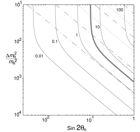
Figure 8: Contours of constant $\sigma(e^{+}e^{-}\to e^{\pm}\mu^{\mp}\tilde{\chi}^{0}_{1}\tilde{\chi}^{0}_{1})$ in fb at a $\sqrt{s}=500$ GeV $e^{+}e^{-}_{R}$ collider. The signal arises from right-slepton production and subsequent decay to lepton plus lightest neutralino. The $\widetilde{\ell}_{R}$ masses are approximately 200 GeV and the lightest neutralino is a Bino with mass 100 GeV. The thick gray contour represents optimal experimental reach with $50\,{\rm fb}^{-1}$ integrated luminosity. The straight lines (dotted and dashed) represent contours of constant $B(\mu\to e\gamma)$. These depend on additional parameters such as the $\widetilde{\ell}_{L}$ mass and the off-diagonal entries of the slepton mass matrix. See [221] for more details.

Direct production of sleptons and close scrutiny of their decays allow probing of these flavor angles at more sensitive levels [221, 222, 223, 224, 225, 226]. The nearly degenerate sleptons will undergo flavor oscillation after being produced and then decay quickly. Analogous to neutrino oscillations, the detectability of slepton oscillations is best characterized in the $(\sin 2\theta,\,\Delta m^{2})$ plane, where $\theta$ is the angle between the weak eigenstates $|\tilde{e}\rangle$, $|\tilde{\mu}\rangle$ and the mass eigenstates $|1\rangle$, $|2\rangle$:

$$|\tilde{e}\rangle=+\cos\theta|1\rangle+\sin\theta|2\rangle$$ (11)

$$|\tilde{\mu}\rangle=-\sin\theta|1\rangle+\cos\theta|2\rangle.$$

Figure 8 shows contours of constant $\sigma(e^{+}e^{-}\to e^{\pm}\mu^{\mp}\tilde{\chi}^{0}_{1}\tilde{\chi}^{0}_{1})$, in fb, at a $\sqrt{s}=500$ GeV collider with $e^{+}e^{-}_{R}$ collisions. The signal arises from $\widetilde{\ell}_{R}$ production and subsequent decay to a lepton plus the lightest neutralino. The $\widetilde{\ell}_{R}$ masses are approximately 200 GeV, and the lightest neutralino is a Bino with mass 100 GeV. From this figure we can see that careful measurement of the cross section enables probing of flavor-violating couplings to very small mass splitting and mixing angle.

3 CP violation

The new mass parameters associated with supersymmetry may not all be real, and could lead to CP violation effects [227] at high-energy colliders. The parameters $\mu$, $M_{1}$ and $M_{2}$ can in general be complex. By rotating the phases of the gauginos we are free to choose $M_{2}$ real, leaving us with

$$\mu=|\mu|e^{i\phi_{\mu}}~{}~{}~{}~{}{\rm and}~{}~{}~{}~{}M_{1}\to|M_{1}|e^{i\phi_{1}}.$$ (12)

In addition to these phases, each of the tri-scalar $A$ terms connecting the Higgs bosons with left and right scalar superpartners of the fermions can in principle have its own independent phase.

Generic ${\cal O}(1)$ phases associated with superpartner masses near the weak scale are ruled out by the electric dipole moments (EDMs) of the neutron and electron if superpartners are light enough to be accessible at a 1 TeV linear collider. Therefore, we assume here that the phases must be small, ${\cal O}(0.1)$. We remark that tuned cancellations [228, 229] may allow ${\cal O}(1)$ phases for light superpartners, thereby leading to effects much larger than the estimates given below.

Supersymmetric CP-violating phases have two important effects: they disrupt the relations among CP-conserving observables, and they give birth to non-zero CP-violating observables. Much work has gone into both types of analyses. For example, CP-violating observables in $e^{+}e^{-}\to t\overline{t}$ may be the most promising way to find actual CP violation effects at the linear collider. We refer the reader to [230, 231, 232] for a comprehensive review of this subject, and a description of the challenges facing experiment to confirm CP-violating effects. Here, we briefly focus on the effects that small phases have on CP-conserving observables.

Recently several groups have shown how CP-violating phases affect almost all interesting MSSM observables at a linear collider [233, 234, 235, 181, 236]. For example, the chargino mass eigenstates depend non-trivially on the phase of $\mu$:

$$m^{2}_{\tilde{\chi}^{\pm}_{1,2}}=\frac{1}{2}\left[M_{2}^{2}+|\mu|^{2}+2m^{2}_{W}\mp\Delta_{C}\right],$$ (13)

where

$$\Delta_{C} = \left[(M^{2}_{2}-|\mu|^{2})^{2}+4m_{W}^{4}\cos^{2}2\beta+4m^{2}_{W}(M_{2}^{2}+|\mu|^{2})\right.$$ (14)

$$+\left.8m_{W}^{2}M_{2}|\mu|\sin 2\beta\cos\Phi_{\mu}\right]^{1/2}.$$

The effects of phases on observables have been illustrated in [236] with a reference model corresponding to an mSUGRA point with $m_{1/2}=200~{}{\rm\,GeV}$, $m_{0}=100~{}{\rm\,GeV}$, $A_{0}=0$, $\tan\beta=4$, and $\mu>0$. This parameter choice corresponds to the mass values $|M_{1}|=83~{}{\rm\,GeV}$, $M_{2}=165~{}{\rm\,GeV}$, $\mu=310~{}{\rm\,GeV}$, $m_{\tilde{e}_{L}}=180~{}{\rm\,GeV}$, $m_{\tilde{\nu}}=166~{}{\rm\,GeV}$, and $m_{\tilde{e}_{R}}=132~{}{\rm\,GeV}$. In Fig. 10, the effects of varying the phases $\phi_{1}$ and $\phi_{\mu}$ are demonstrated for several observables.

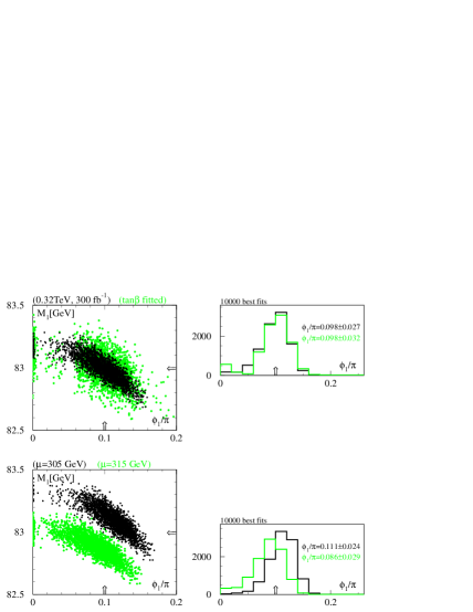
Figure 9: The effects on supersymmetry observables obtained by varying the phases $\phi_{1}$ and $\phi_{\mu}$ in the example model discussed in the text [236].

Figure 10: Demonstration of the interdependence of parameters in the extraction of CP-violating phases from linear collider SUSY observables [236].

Motivated by the EDM constraints on the phases of supersymmetric mass parameters, the authors of [236] set $\phi_{\mu}=0$ and simulated how evidence for a small but non-zero $\phi_{1}$ phase would be extracted at a linear collider. They generated 10000 data sets, smeared with respect to the true values by experimental resolution. The input data included three cross sections ($\tilde{\chi}^{0}_{1}\tilde{\chi}^{0}_{2}$, $\tilde{\chi}^{0}_{2}\tilde{\chi}^{0}_{2}$, and $\tilde{\chi}^{\pm}_{1}\tilde{\chi}^{\mp}_{1}$) and three masses ($m_{\tilde{\chi}^{0}_{1}}$, $m_{\tilde{\chi}^{0}_{2}}$, and $m_{\tilde{\chi}^{\pm}_{1}}$). Figure 10 demonstrates the extraction of several different parameters, and their interdependence. For example, the bottom figures show the systematic error one would encounter by having a wrong input for $|\mu|$ given a known $\tan\beta$. Perhaps the most interesting conclusion one can draw from this exercise is that $\phi_{1}=0$ is strongly disfavored, incicating that the linear collider measurements of CP-conserving observables can give a strong signal for nonzero CP-violating phases if they are present.

6 Supersymmetry and $e^{-}e^{-}$, $e^{-}\gamma$, and $\gamma\gamma$ colliders

1 Supersymmetry and $e^{-}e^{-}$ colliders

The features of $e^{-}e^{-}$ colliders are reviewed in Chapter 14. The unique quantum numbers of the $e^{-}e^{-}$ initial state forbid the production of most superpartners. However, slepton pair production through $t$-channel neutralino exchange is always possible [237]. The opportunities at $e^{-}e^{-}$ colliders for measurements of slepton masses, mixings, and couplings are unparalleled, and exploit many of the unique properties of $e^{-}e^{-}$ colliders.

Masses

As reviewed in Section 2, masses at linear colliders are most accurately determined through kinematic endpoints and threshold scans. In $e^{+}e^{-}$ mode, the threshold cross section for pair production of identical scalars rises as $\beta^{3}$, where $\beta$ is the velocity of the produced particles. Threshold studies for identical scalars are therefore far less effective than for fermions, and consequently require large investments of integrated luminosity [174].

At $e^{-}e^{-}$ colliders, however, the same-helicity selectron pair production cross section has a $\beta$ dependence at threshold [238]. This is easily understood: the initial state in $e^{-}_{R}e^{-}_{R}\to\tilde{e}^{-}_{R}\tilde{e}^{-}_{R}$ has angular momentum $J=0$, and so the selectrons may be produced in the S wave state. Cross sections for $\tilde{e}_{R}$ pair production in $e^{-}e^{-}$ and $e^{+}e^{-}$ modes are compared in Fig. 11. For round beams, the increased beamstrahlung and decreased luminosity of the $e^{-}e^{-}$ mode compromise this advantage. However, beamstrahlung is reduced for flat beams [239], and mass measurements of order 100 MeV can be achieved with two orders of magnitude less luminosity than required in $e^{+}e^{-}$ collisions [240, 241]. Incidentally, the full arsenal of linear collider modes allows one to extend this mass measurement to the rest of the first-generation sleptons through a series of $\beta$ threshold scans: $e^{-}e^{-}\to\tilde{e}^{-}_{R}\tilde{e}^{-}_{R}$ yields $m_{\tilde{e}_{R}}$; $e^{+}e^{-}\to\tilde{e}^{\pm}_{R}\tilde{e}^{\mp}_{L}$ yields $m_{\tilde{e}_{L}}$; $e^{+}e^{-}\to\tilde{\chi}^{+}_{1}\tilde{\chi}^{-}_{1}$ yields $m_{\tilde{\chi}^{\pm}_{1}}$; and $e^{-}\gamma\to\tilde{\nu}_{e}\tilde{\chi}^{-}_{1}$ yields $m_{\tilde{\nu}_{e}}$ [242]. The process $e^{-}e^{-}\to\tilde{e}^{-}_{R}\tilde{e}^{-}_{R}$ may also be used to determine the Bino mass $M_{1}$ with high accuracy even for very large $M_{1}$ [238, 241].

Figure 11: Threshold behavior for $\sigma(e^{-}e^{-}\to\tilde{e}_{R}^{-}\tilde{e}_{R}^{-})$ (upper two contours) and $\sigma(e^{+}e^{-}\to\tilde{e}_{R}^{+}\tilde{e}_{R}^{-})$ (lower two contours) for $m_{\tilde{e}_{R}}=150~{}{\rm GeV}$ and $M_{1}=100~{}{\rm GeV}$ [240]. In each pair, the dotted curve neglects all beam effects, and the solid curve includes the initial state radiation, beamstrahlung, and beam energy spread for flat beams. Results for $e^{-}e^{-}$ round beams (dashed) are also shown. The selectron width is included, and beam polarizations $P_{e^{-}}=0.8$ and $P_{e^{+}}=0$ are assumed.

Mixings

Now that neutrinos are known to mix, lepton flavor is no longer a perfect symmetry. Sleptons may also have inter-generational mixings. Such mixing leads to decays $\tilde{e}\to\mu\tilde{\chi}^{0}_{1},\tau\tilde{\chi}^{0}_{1}$ and may be searched for at either $e^{+}e^{-}$ or $e^{-}e^{-}$ colliders.

At $e^{+}e^{-}$ colliders, the signal is $e^{+}e^{-}\to e^{\pm}\mu^{\mp}\tilde{\chi}^{0}_{1}\tilde{\chi}^{0}_{1},~{}e^{\pm}\tau^{\mp}\tilde{\chi}^{0}_{1}\tilde{\chi}^{0}_{1}$. The backgrounds are $e^{+}e^{-}\to W^{+}W^{-}$, $e^{+}e^{-}\to\nu\nu W^{+}W^{-}$, $e^{+}e^{-}\to e^{\pm}\nu W^{\mp}$, and $\gamma\gamma\to W^{+}W^{-}$. The first two backgrounds may be reduced by $e^{-}_{R}$ beam polarization; however, the last two are irreducible.

In the $e^{-}e^{-}$ case, the signal is $e^{-}e^{-}\to e^{-}\mu^{-}\tilde{\chi}^{0}_{1}\tilde{\chi}^{0}_{1},~{}e^{-}\tau^{-}\tilde{\chi}^{0}_{1}\tilde{\chi}^{0}_{1}$. Among potential backgrounds, $e^{-}e^{-}\to W^{-}W^{-}$ is forbidden by total lepton number conservation, $e^{-}e^{-}\to\nu\nu W^{-}W^{-}$ and $e^{-}e^{-}\to e^{-}\nu W^{-}$ may be suppressed by right-polarizing both $e^{-}$ beams, and $\gamma\gamma\to W^{+}W^{-}$ does not yield two like-sign leptons. As a result, the sensitivity of $e^{-}e^{-}$ colliders to slepton flavor violation is much greater than at $e^{+}e^{-}$ colliders, and probes regions of parameter space beyond current and near-future low-energy experiments searching for $\mu$-$e$ and $\tau$-$e$ transitions [221, 222].

Couplings

The excellent properties of $e^{-}e^{-}$ colliders are also ideal for exploring selectron gauge couplings. As noted in Section 4, precise comparisons of the $e\tilde{e}\tilde{B}$ and $eeB$ couplings provide a model-independent test of supersymmetry. The $e\tilde{e}\tilde{B}$ coupling is a non-decoupling observable sensitive to arbitrarily heavy superpartners. The nearly background-free environment of $e^{-}e^{-}$ colliders makes possible extremely precise measurements of selectron couplings, surpassing those available at $e^{+}e^{-}$ colliders [194], and may help set the scale for far-future colliders in scenarios where some superpartners are extremely heavy.

2 Supersymmetry and $e^{-}\gamma$ colliders

Even if several neutralinos and charginos have light masses such that they can be produced in pairs at the LC, the sleptons might be above threshold for pair production in $e^{+}e^{-}$ collisions. In this case, the sleptons may be accessible in the $e^{-}\gamma$ colliding option in the single-slepton plus lighter-neutralino final state $\tilde{\chi}^{0}_{i}\tilde{e}_{L,R}$.

This reaction was studied in [243, 244, 242]. For example, the parameters chosen in  [242] lead to the masses: $m_{\tilde{\chi}^{0}_{1}}=65$ GeV, $m_{\tilde{\chi}^{\pm}_{1}}=136$ GeV, $m_{\tilde{e}_{L}}=320$ GeV, $m_{\tilde{e}_{R}}=307$ GeV, and $m_{\tilde{\nu}_{e}}=315$ GeV. With these values, pair production of charginos is accessible at a 500 GeV linear collider but slepton pair production is not.

Figure 12 shows the cross sections for slepton-neutralino production as a function of the $e^{-}\gamma$ center-of-mass energy for the four different helicity combinations of the incoming electron and photon. The cross section for $\tilde{e}_{R}\tilde{\chi}^{0}_{1}$ in the $(+,+)$ helicity combination is sharply peaked at center-of-mass energies not far from the threshold. The signal for this process is $e^{-}$ plus missing energy. The background [243, 242] has a cross section of a few picobarns and mainly arises from $W^{-}\nu\to e^{-}\nu\nu$. This background can be reduced dramatically by using a polarized $e^{-}_{R}$ beam. With the above parameters, using polarization and a few judicious kinematic cuts on the final state particles, the slepton can be discovered and studied. It has been estimated that both the slepton and sneutrino masses can be measured to about 1% accuracy.

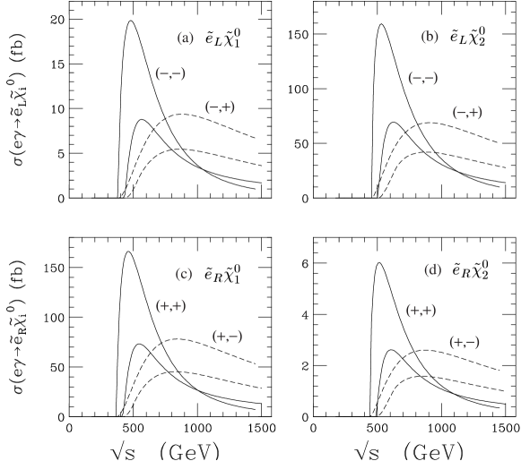
Figure 12: Cross sections for $e^{-}\gamma\to\widetilde{e}\widetilde{\chi}^{0}$ processes, from [242]. The upper two curves show the total cross section (in fb) for $e^{-}\gamma\to\tilde{e}\tilde{\chi}^{0}$ versus $\sqrt{s_{e\gamma}}$ (in GeV) for the SUSY and machine parameters given in the text: (a) $\tilde{e}_{L}\tilde{\chi}_{1}^{0}$; (b) $\tilde{e}_{L}\tilde{\chi}_{2}^{0}$; (c) $\tilde{e}_{R}\tilde{\chi}_{1}^{0}$; (d) $\tilde{e}_{R}\tilde{\chi}_{2}^{0}$. The solid curves represent $e$, $\gamma$ helicities $(-,-)$ for (a), (b) and $(+,+)$ for (c), (d). The dashed curves represent helicities $(-,+)$ for (a), (b) and $(+,-)$ for (c), (d). The lower two curves are corresponding results, convoluted with the backscattered photon spectrum, versus $\sqrt{s_{ee}}$.

3 Supersymmetry at $\gamma\gamma$ colliders

One of the main motivations for the $\gamma\gamma$ collider option is to study direct single Higgs production through the $\gamma\gamma h$ coupling. This motivation is especially powerful in supersymmetry since most versions of the theory predict a Higgs boson below about 135 GeV. The motivation is further strengthened by the realization that additional Higgs states exist in supersymmetry that may not be accessible at the LHC or $e^{+}e^{-}$ annihilation but may be visible in single production from $\gamma\gamma$. These issues are discussed in more detail in Chapters 3 and 13.

For direct superpartner pair production, $\gamma\gamma$ collisions also have an important advantage: the unambiguous production mode for superpartners through photons coupled to charge. Knowing exactly how a particle is produced reaps great benefits when analyzing the actual data recorded by the detectors. Production cross sections of superpartners have been calculated most recently by [245, 246]. It has been argued [246] that some observables derived from $\gamma\gamma\to\chi^{\pm}_{1}\chi^{\mp}_{1}$ production are very useful in extracting fundamental parameters of the supersymmetric Lagrangian. The special advantages $\gamma\gamma$ collisions offer supersymmetry deserve additional careful study.

7 Comparison with LHC

If SUSY is relevant to electroweak symmetry breaking, then the arguments summarized in Section 2 suggest that in many models the gluino and some squark masses are less than ${\cal O}(1\,{\rm\,TeV})$. This is also true in most models with SUSY particles visible at a $500\,{\rm\,GeV}$ LC. Gluinos and squarks then dominate the LHC SUSY cross section, which is of order 10 pb. Since they are strongly produced, it is easy to separate SUSY from SM backgrounds provided only that the SUSY decays are distinctive. In the MSUGRA model, these decays produce multiple jets and $\hbox to0.0pt{\hbox to7.95831pt{\hfil/\hfil}\hss}E_{T}$ plus varying numbers of leptons [247]. Figure 13 shows the $5\sigma$ reach in this model at the LHC for an integrated luminosity of $10\,~{}\mbox{fb${}^{-1}$}$ and $100\,~{}\mbox{fb${}^{-1}$}$ [248]. The reach is comfortably more than the expected mass range.

Figure 13: Plot of $5\sigma$ reach with multiple jets plus $\hbox to0.0pt{\hbox to7.95831pt{\hfil/\hfil}\hss}E_{T}$ plus leptons in minimal SUGRA model at LHC for $10\,~{}\mbox{fb${}^{-1}$}$ (left) and $100\,~{}\mbox{fb${}^{-1}$}$ (right) [248]. Also shown are contours of the squark and gluino masses and of the cold dark matter density $\Omega h^{2}$.

While the reach in Fig. 13 has been calculated for a specific SUSY model, the multiple jet plus $\hbox to0.0pt{\hbox to7.95831pt{\hfil/\hfil}\hss}E_{T}$ signature is generic in most R-parity-conserving models. GMSB models can give additional photons or leptons or long-lived sleptons with high $p_{T}$ but $\beta<1$, making the search easier [249, 250]. R-parity-violating models with leptonic $\widetilde{\chi}^{0}_{1}$ decays also give extra leptons and very likely violate $e$-$\mu$ universality. R-parity-violating models with $\widetilde{\chi}^{0}_{1}\to qqq$ give signals at the LHC with very large jet multiplicity, for which the SM background is not well known. For such models, it may be necessary to rely on leptons produced in the cascade decay of the gluinos and squarks. In AMSB models, cascade decays of gluinos and squarks again lead to a substantial reach for SUSY by the LHC [251]. In all cases, it seems likely that SUSY can be discovered at the LHC if the masses are in the expected range [252, 253, 254].

Figure 14: Plot of the $e^{+}e^{-}+\mu^{+}\mu^{-}-e^{\pm}\mu^{\mp}$ mass distribution for LHC SUGRA Point 4 with direct $\widetilde{\chi}^{0}_{2}\to\widetilde{\chi}^{0}_{1}\ell\ell$ decay (left) and for LHC SUGRA Point 5 with $\widetilde{\chi}^{0}_{2}\to\widetilde{\ell}^{\pm}\ell^{\mp}\to\widetilde{\chi}^{0}_{1}\ell^{+}\ell^{-}$ (right) [252]. The event generator ISAJET is used. The shape of the peak on the left plot below 70 GeV should be compared to the shape of the peak in the right plot. The left plot also contains a $Z\to\ell^{+}\ell^{-}$ signal that comes from heavier gauginos.

The main problem at the LHC is not to observe a signal that deviates from the SM but to separate the many different channels produced by all the SUSY cascade decays from the produced squarks [255] and gluinos. One promising approach is to try to identify particular decay chains and to measure kinematic endpoints for combinations of the visible particles in these [256]. For example, the $\ell^{+}\ell^{-}$ mass distribution from $\widetilde{\chi}^{0}_{2}\to\widetilde{\chi}^{0}_{1}\ell^{+}\ell^{-}$ has an endpoint that measures $M_{\widetilde{\chi}^{0}_{2}}-M_{\widetilde{\chi}^{0}_{1}}$ [257], while the distribution from $\widetilde{\chi}^{0}_{2}\to\widetilde{\ell}^{\pm}\ell^{\mp}\to\widetilde{\chi}^{0}_{1}\ell^{+}\ell^{-}$ has a different shape and measures

$$M_{\ell\ell}^{\rm max}=\sqrt{(M_{\widetilde{\chi}^{0}_{2}}^{2}-M_{\widetilde{\ell}}^{2})(M_{\widetilde{\ell}}^{2}-M_{\widetilde{\chi}^{0}_{1}}^{2})\over M_{\widetilde{\ell}}^{2}}\ .$$

The flavor-subtraction combination $e^{+}e^{-}+\mu^{+}\mu^{-}-e^{\pm}\mu^{\mp}$ removes backgrounds from two independent decays. Dilepton mass distributions [252] after cuts for an example of each decay are shown in Fig. 14.

If a longer decay chain can be identified, then more combinations of masses can be measured. Consider, for example, the decay chain

$$\widetilde{q}_{L}\to\widetilde{\chi}^{0}_{2}q\to\widetilde{\ell}_{R}^{\pm}\ell^{\mp}q\to\widetilde{\chi}^{0}_{1}\ell^{+}\ell^{-}q\ .$$

For this decay chain, kinematics gives $\ell^{+}\ell^{-}$, $\ell^{+}\ell q$, and two $\ell q$ endpoints in terms of the masses. If a lower limit is imposed on the $\ell^{+}\ell^{-}$ mass, there is also a $\ell^{+}\ell^{-}q$ lower edge. With suitable cuts all of these can be measured [252, 258] for the cases considered. The statistical errors on the measured endpoints are typically comparable to the systematic limits, ${\cal O}(0.1\%)$ for leptons and ${\cal O}(1\%)$ for jets. Figure 15 shows a scatter plot of the resulting $\widetilde{\ell}_{R}$ and $\widetilde{\chi}^{0}_{1}$ masses for LHC SUGRA Point 5 and for a similar point in another SUSY model with this decay chain [259]. The relations between masses are determined with good precision, so these two models are easily distinguished. However, the LSP mass is only measured to ${\cal O}(10\%)$.

Figure 15: Left: Scatter plot of reconstructed values of the $\widetilde{\ell}_{R}$ and $\widetilde{\chi}^{0}_{1}$ masses for LHC Point 5 (S5) and for a different model (O1) using the decay chain $\widetilde{q}_{L}\to\widetilde{\chi}^{0}_{2}q\to\widetilde{\ell}_{R}\ell q\to\widetilde{\chi}^{0}_{1}\ell\ell q$. Right: Projection of $M_{\widetilde{\chi}^{0}_{1}}$ for LHC Point 5 [259].

Analyses such as these have proved useful for a number of SUSY points in a variety of SUSY models [252]. The method seems fairly general: there is usually at least one distinctive mode — typically $\widetilde{\chi}^{0}_{2}\to\widetilde{\chi}^{0}_{1}\ell^{+}\ell^{-}$, $\widetilde{\chi}^{0}_{2}\to\widetilde{\ell}_{R}^{\pm}\ell^{\mp}$, or $\widetilde{\chi}^{0}_{2}\to\widetilde{\chi}^{0}_{1}h\to\widetilde{\chi}^{0}_{1}b\overline{b}$ — from which to start. But some points are much more difficult than others. For example, in MSUGRA with $\tan\beta\gg 1$ it is possible to choose parameters such that the only allowed 2-body decays of $\widetilde{\chi}^{0}_{2}$ and $\widetilde{\chi}_{1}^{\pm}$ are $\widetilde{\tau}_{1}^{\pm}\tau^{\mp}$ and $\widetilde{\tau}_{1}^{\pm}\nu_{\tau}$ [260] respectively. These modes then have branching ratios in excess of 99%. While it is possible to identify and to measure hadronic $\tau$ decays [252], the measurements are much less precise than those involving leptons. Even if $\tau$ decays are not dominant, they may be important, since they can provide information on $\widetilde{\tau}_{L}-\widetilde{\tau}_{R}$ and gaugino-Higgsino mixing.

If SUSY is found at the LHC, the SUSY events will contain much more information than just endpoints like those described above. For example, while it is not possible to reconstruct $\widetilde{\chi}_{1}^{\pm}$ decays in the same way because of the missing neutrino, one can get information about the chargino mass by studying $M_{\ell q}$ and other distributions for 1-lepton events. Cross sections and branching ratios can also be measured; interpretation of these will be limited by the theoretical errors on the calculation of cross sections and acceptances. Without real experimental data, it is difficult to assess such theoretical systematic errors.

SUSY signatures at the LHC typically come from a combination of many SUSY particles, so the analysis is considerably more complicated than that at a LC. However, the initial steps at the LHC are fairly clear. First, one will look for a deviation from the SM in inclusive distributions such as multiple jets plus $\hbox to0.0pt{\hbox to7.95831pt{\hfil/\hfil}\hss}E_{T}$, perhaps accompanied by leptons and/or photons. If a signal consistent with SUSY is found, it should determine both the mass scale [252, 261] and the qualitative nature of the signal. (As a simple example, in a GMSB model with a long-lived slepton NLSP, SUSY events would contain two high-$p_{T}$ particles with $\beta<1$.) Next, one will look for various kinematic endpoints like those described above and use them further to constrain the SUSY masses. After this, one will look at more model-dependent quantities such as kinematic distributions, cross sections, and branching ratios. These seem difficult to assess without real data.

This program is likely to provide considerable information about gluinos, squarks, and their primary decay products, including $\widetilde{\chi}^{0}_{1}$, $\widetilde{\chi}^{0}_{2}$, $\widetilde{\chi}^{\pm}$, and any sleptons that occur in their decays. It is more dangerous to predict what cannot be done, but there are measurements that appear difficult at the LHC and that could be done at a $500\,{\rm\,GeV}$ LC. For example:

• While it is possible to measure the $\widetilde{\chi}^{0}_{1}$ mass at the LHC in favorable cases, it seems difficult to reduce the error below ${\cal O}(10\%)$. If any visible SUSY particle is produced at a LC, the error on $M_{\widetilde{\chi}^{0}_{1}}$ should be ${\cal O}(1\%)$.

• Sleptons that are not produced in $\widetilde{\chi}^{0}_{2}$ or $\widetilde{\chi}_{1}^{\pm}$ decays are difficult to study at the LHC: both the Drell-Yan process and decays of heavier gauginos typically give very small rates [262]. They can be precisely measured at a LC.

• Distinguishing $\widetilde{\ell}_{L}$ from $\widetilde{\ell}_{R}$ appears very difficult at the LHC except perhaps for $\widetilde{\tau}$’s, but this is straightforward at a LC using the polarized beam.

• Hadronic $\tau$ decays are easier to identify and to measure at a LC because there is no underlying hadronic event.

• Branching ratios currently seem difficult to measure with high precision at the LHC: both the production cross sections and the acceptance have theoretical uncertainties of ${\cal O}(10\%)$. In particular, it seems difficult to make precise tests of SUSY relations among couplings.

More generally, while the LHC seems sure to discover SUSY at the TeV scale if it exists, the measurements of SUSY that can be made there depend on the SUSY model. A LC can provide precise, detailed measurements of any kinematically accessible SUSY particles. Ultimately, one will want such measurements for the entire SUSY spectrum.

References

- [1] J. F. Gunion, H. E. Haber, G. Kane and S. Dawson, The Higgs Hunter’s Guide (Perseus Publishing, Reading, MA, 2000).
- [2] J. F. Gunion, L. Poggioli, R. Van Kooten, C. Kao, P. Rowson et al., “Higgs boson discovery and properties,” in New Directions for High Energy Physics, Proceedings of the 1996 DPF/DPB Summer Study on High Energy Physics, Snowmass ’96, edited by D. G. Cassel, L. T. Gennari and R. H. Siemann (Stanford Linear Accelerator Center, Stanford, CA, 1997) pp. 541–587 [hep-ph/9703330].
- [3] H. E. Haber, T. Han, F. S. Merritt, J. Womersley et al., “Weakly coupled Higgs bosons and precision electroweak physics,” in New Directions for High Energy Physics, Proceedings of the 1996 DPF/DPB Summer Study on High Energy Physics, Snowmass ’96, edited by D. G. Cassel, L. T. Gennari and R. H. Siemann (Stanford Linear Accelerator Center, Stanford, CA, 1997) pp. 482–498 [hep-ph/9703391].
- [4] H. Murayama and M. E. Peskin, Ann. Rev. Nucl. Part. Sci. 46, 533 (1996) [hep-ex/9606003].
- [5] E. Accomando et al. [ECFA/DESY LC Physics Working Group], Phys. Rep. 299, 1 (1998) [hep-ph/9705442].
- [6] For a recent review, see R. N. Mohapatra, “Supersymmetric grand unification: An update,” in Supersymmetry, Supersymmetry and Supercolliders, edited by J. Bagger (World Scientific, 1998) [hep-ph/9911272].
- [7] D. Abbaneo et al. [ALEPH, DELPHI, L3 and OPAL Collaborations, LEP Electroweak Working Group, and SLD Heavy Flavor and Electroweak Groups], CERN-EP-2000-016.
- [8] J. Erler, hep-ph/0102143.
- [9] G. Degrassi, hep-ph/0102137.
- [10] R. Barate et al. [ALEPH Collaboration], Phys. Lett. B495, 1 (2000) [hep-ex/0011045]; P. Abreu et al. [DELPHI Collaboration], Phys. Lett. B499, 23 (2001) [hep-ex/0102036]; M. Acciarri et al. [L3 Collaboration], hep-ex/0012019; G. Abbiendi et al. [OPAL Collaboration], Phys. Lett. B499, 38 (2001) [hep-ex/0101014].
- [11] E. Farhi and L. Susskind, Phys. Rep. 74, 277 (1981); R.K. Kaul, Rev. Mod. Phys. 55, 449 (1983); K. Lane, in The Building Blocks of Creation—From Microfermis to Megaparsecs, Proceedings of the Theoretical Advanced Study Institute (TASI 93) in Elementary Particle Physics, Boulder, CO, 6 June—2 July 1993, edited by S. Raby and T. Walker (World Scientific, Singapore, 1994) [hep-ph/9401324].
- [12] M. E. Peskin and T. Takeuchi, Phys. Rev. Lett. 65, 964 (1990); Phys. Rev. D46, 381 (1992).
- [13] M. E. Peskin and J. D. Wells, hep-ph/0101342.
- [14] A. G. Cohen, in The Building Blocks of Creation—From Microfermis to Megaparsecs, Proceedings of the Theoretical Advanced Study Institute (TASI 93) in Elementary Particle Physics, Boulder, CO, 6 June—2 July 1993, edited by S. Raby and T. Walker (World Scientific, Singapore, 1994).
- [15] The most recent analysis of this type can be found in: T. Hambye and K. Riesselmann, Phys. Rev. D55, 7255 (1997) [hep-ph/9610272].
- [16] The most recent analyses of this type can be found in: G. Altarelli and G. Isidori, Phys. Lett. B337, 141 (1994); J. A. Casas, J. R. Espinosa and M. Quirós, Phys. Lett. B342, 171 (1995) [hep-ph/9409458]; B382, 374 (1996) [hep-ph/9603227].
- [17] R. Dashen and H. Neuberger, Phys. Rev. Lett. 50, 1897 (1983); M. Lüscher and P. Weisz, Phys. Lett. B212, 472 (1988), Nucl. Phys. B318, 705 (1989); U. M. Heller, M. Klomfass, H. Neuberger and P. Vranas, Nucl. Phys. B405, 555 (1993).
- [18] K. Riesselmann, hep-ph/9711456.
- [19] G. ’t Hooft, in Recent Developments in Gauge Theories, Proceedings of the NATO Advanced Summer Institute, Cargese, 1979, edited by G. ’t Hooft et al. (Plenum, New York, 1980) p. 135; E. Witten, Nucl. Phys. B188, 513 (1981); L. Susskind, Phys. Rep. 104, 181 (1984).
- [20] H. P. Nilles, Phys. Rep. 110, 1 (1984).
- [21] H. E. Haber and G. L. Kane, Phys. Rep. 117, 75 (1985); S. P. Martin, hep-ph/9709356.
-
[22]
A. Djouadi, J. Kalinowski and M. Spira,
Comput. Phys. Commun. 108, 56 (1998) [hep-ph/9704448].
The HDECAY program is available at
http://home.cern.ch/~mspira/proglist.html. - [23] A. Djouadi, J. Kalinowski and P. M. Zerwas, Z. Phys. C54, 155 (1992).
- [24] S. Dittmaier, M. Kramer, Y. Liao, M. Spira and P. M. Zerwas, Phys. Lett. B441, 383 (1998) [hep-ph/9808433].
- [25] A. Freitas, W. Hollik, W. Walter and G. Weiglein, Phys. Lett. B495, 338 (2000) [hep-ph/0007091]; A. Freitas, S. Heinemeyer, W. Hollik, W. Walter and G. Weiglein, Nucl. Phys. Proc. Suppl. 89, 82 (2000) [hep-ph/0007129]; hep-ph/0101260.
- [26] J. Erler, S. Heinemeyer, W. Hollik, G. Weiglein and P. M. Zerwas, Phys. Lett. B486, 125 (2000) [hep-ph/0005024].
- [27] M. Carena, J. S. Conway, H. E. Haber and J. D. Hobbs et al., FERMILAB-CONF-00/270-T [hep-ph/0010338].
- [28] M. Dittmar, “LHC luminosity requirements to observe H0 and measure its couplings,” presented at Workshop on the Future of Higgs Physics, Fermilab, Chicago, May 3–5 2001.
- [29] For a recent review, see V. A. Mitsou, ATLAS-CONF-2000-002.
- [30] K. Lassila-Perini, ETH Dissertation thesis No. 12961 (1998).
- [31] D. Zeppenfeld, R. Kinnunen, A. Nikitenko and E. Richter-Wa̧s, Phys. Rev. D62, 013009 (2000) [hep-ph/0002036].
- [32] O. J. Eboli and D. Zeppenfeld, Phys. Lett. B495, 147 (2000) [hep-ph/0009158].
- [33] K. Inoue, A. Kakuto, H. Komatsu, and S. Takeshita, Prog. Theor. Phys. 68, 927 (1982) [E: 70, 330 (1983)]; 71, 413 (1984); R. Flores and M. Sher, Ann. Phys. (NY) 148, 95 (1983).
- [34] J. F. Gunion and H. E. Haber, Nucl. Phys. B272, 1 (1986); B278, 449 (1986) [E: B402, 567 (1993)].
- [35] For a review of the two-Higgs-doublet model (both non-supersymmetric and supersymmetric), see Chapter 4 of [1].
- [36] H. E. Haber and Y. Nir, Phys. Lett. B306, 327 (1993) [hep-ph/9302228]; H. E. Haber, in Physics From the Planck Scale to the Electroweak Scale, Proceedings of the US–Polish Workshop, Warsaw, Poland, September 21–24, 1994, edited by P. Nath, T. Taylor, and S. Pokorski (World Scientific, Singapore, 1995) pp. 49–63 [hep-ph/9501320].
- [37] L. J. Hall and M. B. Wise, Nucl. Phys. B187, 397 (1981).
- [38] H. E. Haber and R. Hempfling, Phys. Rev. Lett. 66, 1815 (1991); Y. Okada, M. Yamaguchi and T. Yanagida, Prog. Theor. Phys. 85, 1 (1991); J. Ellis, G. Ridolfi and F. Zwirner, Phys. Lett. B257, 83 (1991).
- [39] S. Heinemeyer, W. Hollik and G. Weiglein, Phys. Rev. D58, 091701 (1998) [hep-ph/9803277]; Phys. Lett. B440, 296 (1998) [hep-ph/9807423]; Eur. Phys. J. C9, 343 (1999) [hep-ph/9812472]; M. Carena, H. E. Haber, S. Heinemeyer, W. Hollik, C. E. M. Wagner and G. Weiglein, Nucl. Phys. B580, 29 (2000) [hep-ph/0001002]; R.-J. Zhang, Phys. Lett. B447, 89 (1999) [hep-ph/9808299]; J. R. Espinosa and R.-J. Zhang, JHEP 0003, 026 (2000) [hep-ph/9912236]; Nucl. Phys. B586, 3 (2000) [hep-ph/0003246]. The computer programs FeynHiggs and FeynHiggsFast are described respectively in S. Heinemeyer, W. Hollik and G. Weiglein, Comput. Phys. Commun. 124, 76 (2000) [hep-ph/9812320]; CERN-TH-2000-055 [hep-ph/0002213].
- [40] J. Ellis, J. F. Gunion, H. E. Haber, L. Roszkowski and F. Zwirner, Phys. Rev. D39, 844 (1989). For a recent treatment and guide to the literature see: C. Panagiotakopoulos and A. Pilaftsis, Phys. Rev. D 63, 055003 (2001) [hep-ph/0008268]. A detailed discussion of NMSSM phenomenology can be found in U. Ellwanger, M. Rausch de Traubenberg and C. A. Savoy, Nucl. Phys. B492, 21 (1997) [hep-ph/9611251].
- [41] J. R. Espinosa and M. Quirós, Phys. Rev. Lett. 81, 516 (1998) [hep-ph/9804235].
- [42] J. A. Coarasa, R. A. Jiménez and J. Solà, Phys. Lett. B389, 312 (1996) [hep-ph/9511402]; R. A. Jiménez and J. Solà, Phys. Lett. B389, 53 (1996) [hep-ph/9511292]; A. Bartl et al., Phys. Lett. B378, 167 (1996) [hep-ph/9511385].
- [43] L. Hall, R. Rattazzi and U. Sarid, Phys. Rev. D50, 7048 (1994) [hep-ph/9306309]; R. Hempfling, Phys. Rev. D49, 6168 (1994).
- [44] M. Carena, M. Olechowski, S. Pokorski and C. E. M. Wagner, Nucl. Phys. B426, 269 (1994) [hep-ph/9402253].
- [45] D. Pierce, J. Bagger, K. Matchev, and R. Zhang, Nucl. Phys. B491, 3 (1997) [hep-ph/9606211].
- [46] S. Heinemeyer, W. Hollik and G. Weiglein, Eur. Phys. J. C16, 139 (2000) [hep-ph/0003022].
- [47] M. Carena, D. Garcia, U. Nierste and C. E. M. Wagner, Nucl. Phys. B577, 88 (2000) [hep-ph/9912516].
- [48] H. Eberl, K. Hidaka, S. Kraml, W. Majerotto and Y. Yamada, Phys. Rev. D62, 055006 (2000) [hep-ph/9912463].
- [49] M. Carena, S. Mrenna and C.E.M. Wagner, Phys. Rev. D60, 075010 (1999) [hep-ph/9808312]; Phys. Rev. D62, 055008 (2000) [hep-ph/9907422].
- [50] H. Baer and J. D. Wells, Phys. Rev. D57, 4446 (1998) [hep-ph/9710368]; W. Loinaz and J. D. Wells, Phys. Lett. B445, 178 (1998) [hep-ph/9808287].
- [51] J. L. Diaz-Cruz, H.-J. He, T. Tait and C. P. Yuan, Phys. Rev. Lett. 80, 4641 (1998) [hep-ph/9802294]; C. Balázs, J. L. Diaz-Cruz, H.-J. He, T. Tait and C. P. Yuan, Phys. Rev. D59, 055016 (1999) [hep-ph/9807349].
- [52] H. E. Haber et al., Phys. Rev. D63, 055004 (2001) [hep-ph/0007006].
- [53] P. H. Chankowski, S. Pokorski and J. Rosiek, Nucl. Phys. B423, 497 (1994).
- [54] A. Djouadi, P. Janot, J. Kalinowski and P. M. Zerwas, Phys. Lett. B376, 220 (1996) [hep-ph/9603368]; A. Djouadi, J. Kalinowski, P. Ohmann and P. M. Zerwas, Z. Phys. C74, 93 (1997) [hep-ph/9605339].
- [55] S. Heinemeyer, W. Hollik, J. Rosiek and G. Weiglein, Eur. Phys. J. C19, 535 (2001) [hep-ph/0102081].
- [56] J. F. Gunion and H. E. Haber, Phys. Rev. D48, 5109 (1993).
- [57] M. M. Mühlleitner, M. Krämer, M. Spira and P. M. Zerwas, hep-ph/0101083.
- [58] The LEP working group for Higgs boson searches, LHWG note 2001-1 (3 April 2001).
- [59] The ALEPH, DELPHI, L3 and OPAL Collaborations and the LEP Higgs Working Group, LHWG note 2001-2 (26 March 2001).
- [60] The results of Fig. 14 were provided by F. Gianotti on behalf of the ATLAS collaboration. They are the preliminary results available as of March 3, 2001.
- [61] See, for example, J. F. Gunion, hep-ph/9705282.
- [62] S. L. Glashow and S. Weinberg, Phys. Rev. D15, 1958 (1977); E. A. Paschos, Phys. Rev. D15, 1966 (1977).
- [63] B. A. Dobrescu, hep-ph/9903407 and hep-ph/0103038.
- [64] M. Cvetic, H. Lu, C. N. Pope, A. Sadrzadeh and T. A. Tran, Nucl. Phys. B586, 275 (2000) [hep-th/0003103].
- [65] P. Chankowski et al., Phys. Lett. B496, 195 (2000) [hep-ph/0009271].
- [66] J. F. Gunion and H. E. Haber, in preparation.
- [67] U. Ellwanger and C. Hugonie, hep-ph/9909260.
- [68] J. F. Gunion, H. E. Haber and T. Moroi, “Will at least one of the Higgs bosons of the next-to-minimal supersymmetric extension of the Standard Model be observable at LEP2 or the LHC?” in New Directions for High Energy Physics, Proceedings of the 1996 DPF/DPB Summer Study on High Energy Physics, Snowmass ’96, edited by D. G. Cassel, L. T. Gennari and R. H. Siemann (Stanford Linear Accelerator Center, Stanford, CA, 1997) [hep-ph/9610337].
- [69] J. F. Gunion and B. Grzadkowski, work in progress.
- [70] J. R. Espinosa and J. F. Gunion, Phys. Rev. Lett. 82, 1084 (1999) [hep-ph/9807275].
- [71] B. Grzadkowski, J. F. Gunion and J. Kalinowski, Phys. Lett. B480, 287 (2000) [hep-ph/0001093].
- [72] H. E. Haber and Y. Nir, Phys. Lett. B306, 327 (1993) [hep-ph/9302228].
- [73] A. Djouadi, P. M. Zerwas and H. E. Haber, Phys. Lett. B375, 203 (1996) [hep-ph/9602234].
- [74] J. F. Gunion and T. Farris, LC note in preparation.
- [75] M. Battaglia and K. Desch, hep-ph/0101165.
- [76] TESLA Technical Design Report, R. Heuer, D. Miller, F. Richard, A. Wagner and P. M. Zerwas (editors), obtainable from www.desy.de/lcnotes/tdr/ .
-
[77]
See also
http://www-sldnt.slac.stanford.edu/nld/. - [78] H. Yang and K. Riles, “Measurement of Higgs Mass and Cross Section at NLC”, presented at Workshop on Physics and Detectors for Future Linear Colliders, Johns Hopkins University, Baltimore, 19–21 March 2001.
- [79] M. Ronan, “Jet-Jet Reconstruction in Full Detector Simulations”, presented at Workshop on Physics and Detectors for Future Linear Colliders, Johns Hopkins University, Baltimore, 19–21 March 2001.
- [80] A. Juste, hep-ex/9912041.
- [81] V. Barger, M. S. Berger, J. F. Gunion and T. Han, Phys. Rev. Lett. 78, 3991 (1997) [hep-ph/9612279].
- [82] P. F. Derwent et al., FERMILAB-FN-701, report in preparation.
- [83] A. Küskinen, M. Battaglia, P. Pöyhoönen, “Study of at a 800 GeV Linear Collider”, to appear in the Proc. of the Fifth Int. Workshop on Linear Colliders - LCSW2000, Fermilab, October 2000, LC-PHSM-2001-041; A. Andreazza, C. Troncon, “Study of Production in Collisions at GeV, DESY-123-E, p. 417.
- [84] P. Garcia-Abia and W. Lohmann, hep-ex/9908065.
- [85] R. Van Kooten, “Separation of the Higgsstrahlung and -fusion process”, presented at Workshop on Physics and Detectors for Future Linear Colliders, Johns Hopkins University, Baltimore, 19–21 March 2001.
- [86] J. Brau, C. Potter, and M. Iwasaki, “Higgs Branching Ratio Measurements at a Future Linear Collider”, presented at Workshop on Physics and Detectors for Future Linear Colliders, Johns Hopkins University, Baltimore, 19–21 March 2001.
- [87] J. Brau, C. Potter, and M. Iwasaki, “Linear Collider Vertex Detector Optimization for Higgs Branching Ratio Measurements”, LCWS 2000 Proceedings, session D3.
- [88] D. J. Jackson, Nucl. Instrum. Meth. A388, 247 (1997).
- [89] M. D. Hildreth, T. L. Barklow, and D. L. Burke, Phys. Rev. D49, 3441 (1994); K. Kawagoe, UT-ICEPP-93-10, contributed to the 2nd International Workshop on Physics and Experiments with Linear Colliders, Waikoloa, HI, 26–30 April 1993.
- [90] G. Borisov and F. Richard, hep-ph/9905413.
- [91] M. Battaglia, hep-ex/0012021; hep-ph/9910271.
- [92] J. F. Gunion and P. C. Martin, hep-ph/9610417; J. F. Gunion and P. C. Martin, Phys. Rev. Lett. 78, 4541 (1997) [hep-ph/9607360].
- [93] E. Boos, J. C. Brient, D. W. Reid, H. J. Schreiber and R. Shanidze, hep-ph/0011366.
- [94] J. F. Gunion, B. Grzadkowski and X. He, Phys. Rev. Lett. 77, 5172 (1996) [hep-ph/9605326].
- [95] S. Dawson and L. Reina, Phys. Rev. D57, 5851 (1998); D59, 054012 (1999); D60, 015003 (1999); H. Baer, S. Dawson, and L. Reina, Phys. Rev. D61, 0113002 (2000).
- [96] A. Juste and G. Merino, hep-ph/9910301.
- [97] D. J. Miller and S. Moretti, hep-ph/0001194.
- [98] C. Castanier, P. Gay, P. Lutz and J. Orloff, hep-ex/0101028.
- [99] R. Lafaye, D. J. Miller, M. Mühlleitner and S. Moretti, hep-ph/0002238.
- [100] A. Djouadi, W. Kilian, M. Mühlleitner and P. M. Zerwas, hep-ph/0001169.
- [101] M. Carena, H. E. Haber, H. E. Logan and S. Mrenna, FERMILAB-Pub-00/334-T, in preparation.
- [102] J. Alcaraz and E. Ruiz Morales, hep-ph/0012109.
- [103] D. Bardin, P. Christova, M. Jack, L. Kalinovskaya, A. Olchevski, S. Riemann and T. Riemann, Comput. Phys. Commun. 133, 229 (2001) [hep-ph/9908433].
- [104] M. Battaglia and K. Desch, hep-ph/0101165.
- [105] V. Drollinger and A. Sopczak, hep-ph/0102342.
- [106] L. D. Landau, Dokl. Akad. Nauk Ser. Fiz. 60, 207 (1948); C. N. Yang, Phys. Rev. 77, 242 (1950); J.J. Sakurai, Invariance Principles and Elementary Particles (Princeton University Press, 1964).
- [107] D. J. Miller, S. Y. Choi, B. Eberle, M. M. Muhlleitner and P. M. Zerwas, Phys. Lett. B 505, 149 (2001) [hep-ph/0102023].
- [108] K. Hagiwara and M. L. Stong, Z. Phys. C62, 99 (1994) [hep-ph/9309248].
- [109] V. Barger, K. Cheung, A. Djouadi, B. A. Kniehl and P. M. Zerwas, Phys. Rev. D49, 79 (1994) [hep-ph/9306270].
- [110] T. Han and J. Jiang, Phys. Rev. D63, 096007 (2001) [hep-ph/0011271].
- [111] B. Grzadkowski and J. F. Gunion, Phys. Lett. B350, 218 (1995) [hep-ph/9501339].
- [112] B. Grzadkowski and J. F. Gunion, hep-ph/9503409.
- [113] M. Krämer, J. Kühn, M. L. Stong and P. M. Zerwas, Z. Phys. C64, 21 (1994) [hep-ph/9404280].
- [114] J. F. Gunion and X. G. He, hep-ph/9609453.
- [115] B. Grzadkowski and J. F. Gunion, Phys. Lett. B294, 361 (1992) [hep-ph/9206262].
- [116] J. F. Gunion and J. G. Kelly, Phys. Lett. B333, 110 (1994) [hep-ph/9404343].
- [117] C. A. Boe, O. M. Ogreid, P. Osland and J. Zhang, Eur. Phys. J. C9, 413 (1999) [hep-ph/9811505].
- [118] J. F. Gunion and J. Kelly, Phys. Rev. D56, 1730 (1997) [hep-ph/9610495].
- [119] J. F. Gunion and J. Kelly, hep-ph/9610421.
- [120] J. L. Feng and T. Moroi, Phys. Rev. D56, 5962 (1997) [hep-ph/9612333].
- [121] A. Bartl et al., Z. Phys. C76, 549 (1997) [hep-ph/9701336]; hep-ph/9909378; M. Berggren, R. Keränen, H. Nowak and A. Sopczak, hep-ph/9911345.
- [122] S. Y. Choi, A. Djouadi, M. Guchait, J. Kalinowski and P. M. Zerwas, Eur. Phys. J. C14, 535 (2000) [hep-ph/0002033].
- [123] ATLAS Collaboration, “Detector and Physics Performance Technical Design Report”, CERN/LHCC/99-15 (1999); CMS Collaboration, Technical Design Reports, CMS TDR 1-5 (1997/98).
- [124] J. Erler and S. Heinemeyer, hep-ph/0102083.
- [125] I. F. Ginzburg, G. L. Kotkin, V. G. Serbo and V. I. Telnov, Nucl. Instrum. Meth. A205, 47 (1983).
- [126] I. F. Ginzburg, G. L. Kotkin, S. L. Panfil, V. G. Serbo and V. I. Telnov, Nucl. Instrum. Meth. A219, 5 (1984).
-
[127]
P. Chen, G. Horton-Smith, T Ohgaki, A. W. Weidemann and K. Yokoya,
Nucl. Instrum. Meth. A355, 107 (1995).
See
http://www-acc-theory.kek.jp/members/cain/cain21b.manual/main.html. - [128] D. Asner, J. Gronberg, J. Gunion and T. Hill, UCRL–ID–143967.
- [129] S. Söldner-Rembold and G. Jikia, hep-ex/0101056.
- [130] J. F. Gunion, J. G. Kelly and J. Ohnemus, Phys. Rev. D51, 2101 (1995) [hep-ph/9409357].
- [131] J. F. Gunion, R. Vega and J. Wudka, Phys. Rev. D43, 2322 (1991).
- [132] R. N. Mohapatra, Fortsch. Phys. 31, 185 (1983); J. F. Gunion, J. Grifols, A. Mendez, B. Kayser and F. Olness, Phys. Rev. D40, 1546 (1989); N. G. Deshpande, J. F. Gunion, B. Kayser and F. Olness, Phys. Rev. D44, 837 (1991).
- [133] H. Georgi and M. Machacek, Nucl. Phys. B262, 463 (1985).
- [134] M. S. Chanowitz and M. Golden, Phys. Lett. B165, 105 (1985).
- [135] J. F. Gunion, Int. J. Mod. Phys. A11, 1551 (1996) [hep-ph/9510350]; A13, 2277 (1998) [hep-ph/9803222].
- [136] P. H. Frampton, Int. J. Mod. Phys. A15, 2455 (2000) [hep-ph/0002017].
- [137] F. Cuypers and M. Raidal, Nucl. Phys. B501, 3 (1997) [hep-ph/9704224].
- [138] J. Gluza, Phys. Lett. B403, 304 (1997) [hep-ph/9704202].
- [139] R. A. Alanakian, Phys. Lett. B436, 139 (1998) [hep-ph/9706383].
- [140] G. Barenboim, K. Huitu, J. Maalampi and M. Raidal, Phys. Lett. B394, 132 (1997) [hep-ph/9611362].
- [141] V. Barger, J. F. Beacom, K. Cheung and T. Han, Phys. Rev. D50, 6704 (1994) [hep-ph/9404335].
- [142] R. Casalbuoni, A. Deandrea, S. De Curtis, D. Dominici, R. Gatto and J. F. Gunion, Nucl. Phys. B555, 3 (1999) [hep-ph/9809523].

References

- [1] The LEP Collaborations, the LEP Electroweak Working Group, and the SLD Heavy Flavour and Electroweak Working Groups, hep-ex/0103048, CERN-EP/2001-021 (February 28, 2001).
- [2] L. Maiani, in Proc. Gif-sur-Yvette Summer School (Paris, 1980), p. 3.
- [3] M. Veltman, Acta Phys. Polon. B12, 437 (1981).
- [4] E. Witten, Nucl. Phys. B188, 513 (1981).
- [5] R. K. Kaul, Phys. Lett. B109, 19 (1982).
- [6] S. Dimopoulos, S. Raby and F. Wilczek, Phys. Rev. D24, 1681 (1981).
- [7] U. Amaldi et al., Phys. Rev. D36, 1385 (1987).
- [8] P. Langacker and M. Luo, Phys. Rev. D44, 817 (1991).
- [9] J. Bagger, K. Matchev and D. Pierce, Phys. Lett. B348, 443 (1995) [hep-ph/9501277].
- [10] P. Langacker and N. Polonsky, Phys. Rev. D52, 3081 (1995) [hep-ph/9503214].
- [11] H. Goldberg, Phys. Rev. Lett. 50, 1419 (1983).
- [12] C. Ahn et al., High-Energy E+ E- Collider,” SLAC-0329.
- [13] P. M. Zerwas, editor, “E+ E- Collisions At 500-Gev: The Physics Potential. Proceedings, Workshop, Munich, Germany, February 4, 1991, Annecy, France, June 10-11, 1991, Hamburg, Germany, September 2-3, 1991,” DESY-92-123A-B.
- [14] JLC Group Collaboration, KEK-92-16.
- [15] S. Kuhlman et al. [NLC ZDR Design Group and NLC Physics Working Group Collaboration], hep-ex/9605011.
- [16] M. Danielson et al., in New Directions in High Energy Physics, Proc. 1996 Snowmass Summer Study, editors D. Cassel, L. Trindle Gennari and R. H. Siemann (SLAC, 1997).
- [17] S. Abdullin et al., hep-ph/0005142.
- [18] R. D. Heuer, D. Miller, F. Richard and P. Zerwas, DESY-01-011C.
- [19] H. P. Nilles, Phys. Rept. 110 (1984) 1.
- [20] H. E. Haber and G. L. Kane, Phys. Rept. 117 (1985) 75.
- [21] G. F. Giudice and R. Rattazzi, Phys. Rept. 322, 419 (1999) [hep-ph/9801271].
- [22] L. Randall and R. Sundrum, Nucl. Phys. B557, 79 (1999) [hep-th/9810155].
- [23] G. F. Giudice, M. A. Luty, H. Murayama and R. Rattazzi, JHEP 9812, 027 (1998) [hep-ph/9810442].
- [24] J. Ellis, K. Enqvist, D. V. Nanopoulos and F. Zwirner, Mod. Phys. Lett. A1, 57 (1986).
- [25] R. Barbieri and G. F. Giudice, Nucl. Phys. B306, 63 (1988).
- [26] G. G. Ross and R. G. Roberts, Nucl. Phys. B377, 571 (1992).
- [27] B. de Carlos and J. A. Casas, Phys. Lett. B309, 320 (1993) [hep-ph/9303291].
- [28] G. W. Anderson and D. J. Castaño, Phys. Lett. B347, 300 (1995) [hep-ph/9409419].
- [29] G. W. Anderson and D. J. Castaño, Phys. Rev. D52, 1693 (1995) [hep-ph/9412322].
- [30] G. W. Anderson and D. J. Castaño, Phys. Rev. D53, 2403 (1996) [hep-ph/9509212].
- [31] S. Dimopoulos and G. F. Giudice, Phys. Lett. B357, 573 (1995) [hep-ph/9507282].
- [32] A. Pomarol and D. Tommasini, Nucl. Phys. B466, 3 (1996) [hep-ph/9507462].
- [33] K. Agashe and M. Graesser, Nucl. Phys. B507, 3 (1997) [hep-ph/9704206].
- [34] P. Ciafaloni and A. Strumia, Nucl. Phys. B494, 41 (1997) [hep-ph/9611204].
- [35] G. Bhattacharyya and A. Romanino, Phys. Rev. D55, 7015 (1997) [hep-ph/9611243].
- [36] R. Barbieri and A. Strumia, Phys. Lett. B433, 63 (1998) [hep-ph/9801353].
- [37] L. Giusti, A. Romanino and A. Strumia, Nucl. Phys. B550, 3 (1999) [hep-ph/9811386].
- [38] A. Romanino and A. Strumia, Phys. Lett. B487, 165 (2000) [hep-ph/9912301].
- [39] K. L. Chan, U. Chattopadhyay and P. Nath, Phys. Rev. D58, 096004 (1998) [hep-ph/9710473].
- [40] P. H. Chankowski, J. Ellis and S. Pokorski, Phys. Lett. B423, 327 (1998) [hep-ph/9712234].
- [41] P. H. Chankowski, J. Ellis, M. Olechowski and S. Pokorski, Nucl. Phys. B544, 39 (1999) [hep-ph/9808275].
- [42] G. L. Kane and S. F. King, Phys. Lett. B451, 113 (1999) [hep-ph/9810374].
- [43] M. Bastero-Gil, G. L. Kane and S. F. King, Phys. Lett. B474, 103 (2000) [hep-ph/9910506].
- [44] J. L. Feng, K. T. Matchev and T. Moroi, Phys. Rev. Lett. 84, 2322 (2000) [hep-ph/9908309].
- [45] J. L. Feng, K. T. Matchev and T. Moroi, Phys. Rev. D61, 075005 (2000) [hep-ph/9909334].
- [46] J. L. Feng and K. T. Matchev, Phys. Rev. D63, 095003 (2001) [hep-ph/0011356].
- [47] M. Drees, Phys. Rev. D33, 1468 (1986).
- [48] M. Dine, A. Kagan and S. Samuel, Phys. Lett. B243, 250 (1990).
- [49] G. Dvali and A. Pomarol, Phys. Rev. Lett. 77, 3728 (1996) [hep-ph/9607383].
- [50] G. Dvali and A. Pomarol, Nucl. Phys. B522, 3 (1998) [hep-ph/9708364].
- [51] A. G. Cohen, D. B. Kaplan and A. E. Nelson, Phys. Lett. B388, 588 (1996) [hep-ph/9607394].
- [52] R. Zhang, Phys. Lett. B402, 101 (1997) [hep-ph/9702333].
- [53] H. P. Nilles and N. Polonsky, Phys. Lett. B412, 69 (1997) [hep-ph/9707249].
- [54] J. L. Feng, C. Kolda and N. Polonsky, Nucl. Phys. B546, 3 (1999) [hep-ph/9810500].
- [55] J. Bagger, J. L. Feng and N. Polonsky, Nucl. Phys. B563, 3 (1999) [hep-ph/9905292].
- [56] J. A. Bagger, J. L. Feng, N. Polonsky and R. Zhang, Phys. Lett. B473, 264 (2000) [hep-ph/9911255].
- [57] Q. Shafi and Z. Tavartkiladze, Phys. Lett. B473, 272 (2000) [hep-ph/9911264].
- [58] H. Baer, M. A. Díaz, P. Quintana and X. Tata, JHEP 0004, 016 (2000) [hep-ph/0002245].
- [59] H. Baer, C. Balazs, P. Mercadante, X. Tata and Y. Wang, Phys. Rev. D63, 015011 (2001) [hep-ph/0008061].
- [60] H. Baer, C. Balazs, M. Brhlik, P. Mercadante, X. Tata and Y. Wang, hep-ph/0102156.
- [61] J. Hisano, K. Kurosawa and Y. Nomura, Phys. Lett. B445, 316 (1999) [hep-ph/9810411].
- [62] J. Hisano, K. Kurosawa and Y. Nomura, Nucl. Phys. B584, 3 (2000) [hep-ph/0002286].
- [63] D. E. Kaplan and G. D. Kribs, Phys. Rev. D61, 075011 (2000) [hep-ph/9906341].
- [64] J. L. Feng and T. Moroi, Phys. Rev. D61, 095004 (2000) [hep-ph/9907319].
- [65] K. Agashe, Phys. Rev. D61, 115006 (2000) [hep-ph/9910497].
- [66] U. Chattopadhyay, A. Datta, A. Datta, A. Datta and D. P. Roy, Phys. Lett. B493, 127 (2000) [hep-ph/0008228].
- [67] B. C. Allanach, J. P. Hetherington, M. A. Parker and B. R. Webber, JHEP 0008, 017 (2000) [hep-ph/0005186].
- [68] U. Chattopadhyay, T. Ibrahim and D. P. Roy, hep-ph/0012337.
- [69] G. F. Giudice and A. Masiero, Phys. Lett. B206, 480 (1988).
- [70] J. Ellis, J. S. Hagelin, D. V. Nanopoulos and M. Srednicki, Phys. Lett. B127, 233 (1983).
- [71] A. H. Jaffe et al., astro-ph/0007333.
- [72] K. Griest and D. Seckel, Phys. Rev. D43, 3191 (1991).
- [73] P. Gondolo and G. Gelmini, Nucl. Phys. B360, 145 (1991).
- [74] P. Nath and R. Arnowitt, Phys. Rev. Lett. 70, 3696 (1993) [hep-ph/9302318].
- [75] S. Mizuta and M. Yamaguchi, Phys. Lett. B298, 120 (1993) [hep-ph/9208251].
- [76] J. Ellis, T. Falk and K. A. Olive, Phys. Lett. B444, 367 (1998) [hep-ph/9810360].
- [77] M. E. Gomez, G. Lazarides and C. Pallis, Phys. Rev. D61, 123512 (2000) [hep-ph/9907261].
- [78] M. Drees and M. M. Nojiri, Phys. Rev. D47, 376 (1993) [hep-ph/9207234].
- [79] K. A. Olive and M. Srednicki, Phys. Lett. B230, 78 (1989).
- [80] K. Griest, M. Kamionkowski and M. S. Turner, Phys. Rev. D41, 3565 (1990).
- [81] K. A. Olive and M. Srednicki, Nucl. Phys. B355, 208 (1991).
- [82] J. L. Lopez, K. Yuan and D. V. Nanopoulos, Phys. Lett. B267, 219 (1991).
- [83] S. Kelley, J. L. Lopez, D. V. Nanopoulos, H. Pois and K. Yuan, Phys. Rev. D47, 2461 (1993) [hep-ph/9207253].
- [84] R. G. Roberts and L. Roszkowski, Phys. Lett. B309, 329 (1993) [hep-ph/9301267].
- [85] G. L. Kane, C. Kolda, L. Roszkowski and J. D. Wells, Phys. Rev. D49, 6173 (1994) [hep-ph/9312272].
- [86] H. Baer and M. Brhlik, Phys. Rev. D53, 597 (1996) [hep-ph/9508321].
- [87] R. Arnowitt and P. Nath, Phys. Lett. B437, 344 (1998) [hep-ph/9801246].
- [88] S. Abdullin and F. Charles, Nucl. Phys. B547, 60 (1999) [hep-ph/9811402].
- [89] J. Ellis, G. Ganis and K. A. Olive, Phys. Lett. B474, 314 (2000) [hep-ph/9912324].
- [90] M. Drees, M. M. Nojiri, D. P. Roy and Y. Yamada, Phys. Rev. D56, 276 (1997) [hep-ph/9701219].
- [91] V. Barger and C. Kao, Phys. Rev. D57, 3131 (1998) [hep-ph/9704403].
- [92] C. Boehm, A. Djouadi and M. Drees, Phys. Rev. D62, 035012 (2000) [hep-ph/9911496].
- [93] A. Bottino, F. Donato, N. Fornengo and S. Scopel, Phys. Rev. D62, 056006 (2000) [hep-ph/0001309].
- [94] J. L. Feng, K. T. Matchev and F. Wilczek, Phys. Lett. B482, 388 (2000) [hep-ph/0004043].
- [95] J. L. Feng, K. T. Matchev and F. Wilczek, Phys. Rev. D63, 045024 (2001) [astro-ph/0008115].
- [96] H. Baer, M. Brhlik, M. A. Díaz, J. Ferrandis, P. Mercadante, P. Quintana and X. Tata, Phys. Rev. D63, 015007 (2001) [hep-ph/0005027].
- [97] J. Ellis, T. Falk, G. Ganis, K. A. Olive and M. Srednicki, hep-ph/0102098.
- [98] T. Moroi and L. Randall, Nucl. Phys. B570, 455 (2000) [hep-ph/9906527].
- [99] B. Murakami and J. D. Wells, hep-ph/0011082.
- [100] A. Birkedal-Hansen and B. D. Nelson, hep-ph/0102075.
- [101] H. E. Haber and R. Hempfling, Phys. Rev. Lett. 66, 1815 (1991).
- [102] M. S. Berger, Phys. Rev. D41, 225 (1990).
- [103] Y. Okada, M. Yamaguchi and T. Yanagida, Prog. Theor. Phys. 85, 1 (1991).
- [104] J. Ellis, G. Ridolfi and F. Zwirner, Phys. Lett. B257, 83 (1991).
- [105] R. Barbieri and M. Frigeni, Phys. Lett. B258, 395 (1991).
- [106] H. E. Haber and R. Hempfling, Phys. Rev. D48, 4280 (1993) [hep-ph/9307201].
- [107] P. Chankowski, S. Pokorski and J. Rosiek, Nucl. Phys. B423, 437 (1994) [hep-ph/9303309].
- [108] A. Dabelstein, Z. Phys. C67, 495 (1995) [hep-ph/9409375].
- [109] A. Dabelstein, Nucl. Phys. B456, 25 (1995) [hep-ph/9503443].
- [110] D. M. Pierce, J. A. Bagger, K. Matchev and R. Zhang, Nucl. Phys. B491, 3 (1997) [hep-ph/9606211].
- [111] S. Heinemeyer, W. Hollik and G. Weiglein, Phys. Rev. D58, 091701 (1998) [hep-ph/9803277].
- [112] S. Heinemeyer, W. Hollik and G. Weiglein, Phys. Lett. B440, 296 (1998) [hep-ph/9807423].
- [113] S. Heinemeyer, W. Hollik and G. Weiglein, Eur. Phys. J. C9, 343 (1999) [hep-ph/9812472].
- [114] S. Heinemeyer, W. Hollik and G. Weiglein, Phys. Lett. B455, 179 (1999) [hep-ph/9903404].
- [115] M. Carena, H. E. Haber, S. Heinemeyer, W. Hollik, C. E. Wagner and G. Weiglein, Nucl. Phys. B580, 29 (2000) [hep-ph/0001002].
- [116] J. A. Casas, J. R. Espinosa, M. Quiros and A. Riotto, Nucl. Phys. B436, 3 (1995) [hep-ph/9407389].
- [117] M. Carena, J. R. Espinosa, M. Quiros and C. E. Wagner, Phys. Lett. B355, 209 (1995) [hep-ph/9504316].
- [118] M. Carena, M. Quiros and C. E. Wagner, Nucl. Phys. B461, 407 (1996) [hep-ph/9508343].
- [119] H. E. Haber, R. Hempfling and A. H. Hoang, Z. Phys. C75, 539 (1997) [hep-ph/9609331].
- [120] R. Hempfling and A. H. Hoang, Phys. Lett. B331, 99 (1994) [hep-ph/9401219].
- [121] R. Zhang, Phys. Lett. B447, 89 (1999) [hep-ph/9808299].
- [122] J. R. Espinosa and R. Zhang, Nucl. Phys. B586, 3 (2000) [hep-ph/0003246].
- [123] M. Acciarri et al. [L3 Collaboration], Phys. Lett. B495, 18 (2000) [hep-ex/0011043].
- [124] R. Barate et al. [ALEPH Collaboration], Phys. Lett. B495, 1 (2000) [hep-ex/0011045].
- [125] G. Abbiendi et al. [OPAL Collaboration], Phys. Lett. B499, 38 (2001) [hep-ex/0101014].
- [126] P. Abreu et al. [DELPHI Collaboration], Phys. Lett. B499, 23 (2001) [hep-ex/0102036].
- [127] J. Ellis, G. Ganis, D. V. Nanopoulos and K. A. Olive, hep-ph/0009355.
- [128] S. Su, Nucl. Phys. B573, 87 (2000) [hep-ph/9910481].
- [129] G. L. Kane, S. F. King and L. Wang, hep-ph/0010312.
- [130] A. Djouadi, P. Gambino, S. Heinemeyer, W. Hollik, C. Junger and G. Weiglein, Phys. Rev. Lett. 78, 3626 (1997) [hep-ph/9612363].
- [131] A. Djouadi, P. Gambino, S. Heinemeyer, W. Hollik, C. Junger and G. Weiglein, Phys. Rev. D57, 4179 (1998) [hep-ph/9710438].
- [132] J. Erler and D. M. Pierce, Nucl. Phys. B526, 53 (1998) [hep-ph/9801238].
- [133] G. Cho and K. Hagiwara, Nucl. Phys. B574, 623 (2000) [hep-ph/9912260].
- [134] G. Cho, K. Hagiwara and M. Hayakawa, Phys. Lett. B478, 231 (2000) [hep-ph/0001229].
- [135] J. Erler, S. Heinemeyer, W. Hollik, G. Weiglein and P. M. Zerwas, Phys. Lett. B486, 125 (2000) [hep-ph/0005024].
- [136] H. N. Brown et al. [Muon g-2 Collaboration], Phys. Rev. Lett. 86, 2227 (2001) [hep-ex/0102017].
- [137] J. A. Grifols and A. Mendez, Phys. Rev. D26, 1809 (1982).
- [138] J. Ellis, J. Hagelin and D. V. Nanopoulos, Phys. Lett. B116, 283 (1982).
- [139] R. Barbieri and L. Maiani, Phys. Lett. B117, 203 (1982).
- [140] D. A. Kosower, L. M. Krauss and N. Sakai, Phys. Lett. B133, 305 (1983).
- [141] T. C. Yuan, R. Arnowitt, A. H. Chamseddine and P. Nath, Z. Phys. C26, 407 (1984).
- [142] A. Czarnecki and W. J. Marciano, hep-ph/0102122.
- [143] L. Everett, G. L. Kane, S. Rigolin and L. Wang, hep-ph/0102145.
- [144] J. L. Feng and K. T. Matchev, Phys. Rev. Lett. 86, 3480 (2001) [hep-ph/0102146].
- [145] E. A. Baltz and P. Gondolo, hep-ph/0102147.
- [146] U. Chattopadhyay and P. Nath, hep-ph/0102157.
- [147] S. Komine, T. Moroi and M. Yamaguchi, hep-ph/0102204.
- [148] H. Baer, C. Balazs, J. Ferrandis and X. Tata, hep-ph/0103280.
- [149] J. Hisano and K. Tobe, hep-ph/0102315.
- [150] T. Ibrahim, U. Chattopadhyay and P. Nath, hep-ph/0102324.
- [151] J. Ellis, D. V. Nanopoulos and K. A. Olive, hep-ph/0102331.
- [152] K. Choi, K. Hwang, S. K. Kang, K. Y. Lee and W. Y. Song, hep-ph/0103048.
- [153] S. P. Martin and J. D. Wells, hep-ph/0103067.
- [154] T. Tsukamoto, K. Fujii, H. Murayama, M. Yamaguchi, and Y. Okada, Phys. Rev. D51, 3153 (1995).
- [155] J. L. Feng, M. E. Peskin, H. Murayama and X. Tata, Phys. Rev. D52, 1418 (1995) [hep-ph/9502260].
- [156] D. G. Cassel, L. Trindle Gennari, R. H. Siemann, editors “DPF/DPB Summer Study on New Directions for High-Energy Physics (Snowmass 96), Snowmass, CO, 25 Jun - 12 Jul 1996. NEW DIRECTIONS FOR HIGH-ENERGY PHYSICS: Proceedings.”
- [157] E. Goodman, COLO-HEP-398, http://hep-www.colorado.edu/SUSY.
- [158] H. Baer, F. E. Paige, S. D. Protopopescu and X. Tata, hep-ph/0001086.
- [159] J. Dunn, “Study of the Detector Response to a Selectron Signal at the NLC,” COLO-HEP-461, in preparation.
- [160] E. Goodman, COLO-HEP-455, http://hep-www.colorado.edu/SUSY.
- [161] B. Williams, COLO-HEP-402, http://hep-www.colorado.edu/SUSY.
- [162] N. Danielson, COLO-HEP-404, http://hep-www.colorado.edu/SUSY.
- [163] H. Baer, R. Munroe and X. Tata, Phys. Rev. D54, 6735 (1996) [hep-ph/9606325].
- [164] “Supersymmetry, Chapter 3 of TESLA TDR”, DESY-2001-011, ECFA-2001-209.
- [165] J. Barron “Finding the Mass of the Chargino and the Sneutrino at the NLC,” COLO-HEP-459, in preparation.
- [166] C. Veeneman “Study of the Decay with decays ql+l- at the NLC,”COLO-HEP-463, in preparation.
- [167] M. Dima, “Susy / Studies, COLO-HEP-454,” Talk presented at LCWS 2000, Fermilab, October, 2000; http://hep-www.colorado.edu/SUSY.
- [168] N. Danielson and E. Goodman, COLO-HEP-422, http://hep-www.colorado.edu/SUSY.
- [169] T. W. Markiewicz, T. Maruyama, “Interaction region issues at the NLC,” Proceedings of the Worldwide Study on Physics and Experiments with Future Linear e+e- Linear Colliders, Sitges, Barcelona, Spain, April 1999.
- [170] N. Danielson and B. Newman, COLO-HEP-428, http://hep-www.colorado.edu/SUSY.
- [171] R. Kelly and C. Takeuchi, COLO-HEP-450, http://hep-www.colorado.edu/SUSY.
- [172] J. Barron, COLO-HEP-449, http://hep-www.colorado.edu/SUSY.
- [173] D. Staszak,“Studies of a Smuon Signal in a NLC Detector,” COLO-HEP-460, in preparation.
- [174] H. Martyn and G. A. Blair, hep-ph/9910416.
- [175] J. L. Feng and D. E. Finnell, Phys. Rev. D49, 2369 (1994) [hep-ph/9310211].
- [176] David Wagner, COLO-HEP-400, http://hep-www.colorado.edu/SUSY.
- [177] David Wagner, COLO-HEP-401, http://hep-www.colorado.edu/SUSY.
- [178] H. Baer, J. K. Mizukoshi, and X. Tata, private communication.
- [179] J. F. Gunion and S. Mrenna, hep-ph/0103167.
- [180] H. Baer, C. Balazs, S. Hesselbach, J. K. Mizukoshi and X. Tata, hep-ph/0012205.
- [181] S. Y. Choi, A. Djouadi, M. Guchait, J. Kalinowski, H. S. Song and P. M. Zerwas, Eur. Phys. J. C14, 535 (2000) [hep-ph/0002033].
- [182] G. Moortgat-Pick, A. Bartl, H. Fraas and W. Majerotto, Eur. Phys. J. C18, 379 (2000) [hep-ph/0007222].
- [183] M. M. Nojiri, K. Fujii and T. Tsukamoto, Phys. Rev. D54, 6756 (1996) [hep-ph/9606370].
- [184] A. Bartl, H. Eberl, S. Kraml, W. Majerotto, W. Porod and A. Sopczak, Z. Phys. C76, 549 (1997) [hep-ph/9701336].
- [185] H. Baer, C. Balazs, J. K. Mizukoshi and X. Tata, Phys. Rev. D63, 055011 (2001) [hep-ph/0010068].
- [186] M. M. Nojiri, K. Fujii and T. Tsukamoto, Prepared for 6th Workshop on the Japan Linear Collider (JLC), Tokyo, Japan, 4-5 Dec 1996, Phys. Rev. D54, 6756 (1886).
- [187] K. Hikasa and T. Nagano, Phys. Lett. B435, 67 (1998) [hep-ph/9805246].
- [188] J. L. Feng and T. Moroi, Phys. Rev. D56, 5962 (1997) [hep-ph/9612333].
- [189] V. Barger, T. Han and J. Jiang, hep-ph/0006223.
- [190] K. Hikasa and Y. Nakamura, Z. Phys. C70, 139 (1996) [hep-ph/9501382]; erratum, Z. Phys. C71, 356 (1996).
- [191] P. H. Chankowski, Phys. Rev. D41, 2877 (1990).
- [192] M. E. Peskin and T. Takeuchi, Phys. Rev. Lett. 65, 964 (1990).
- [193] H. Cheng, J. L. Feng and N. Polonsky, Phys. Rev. D56, 6875 (1997) [hep-ph/9706438].
- [194] H. Cheng, J. L. Feng and N. Polonsky, Phys. Rev. D57, 152 (1998) [hep-ph/9706476].
- [195] M. M. Nojiri, D. M. Pierce and Y. Yamada, Phys. Rev. D57, 1539 (1998) [hep-ph/9707244].
- [196] E. Katz, L. Randall and S. Su, Nucl. Phys. B536, 3 (1998) [hep-ph/9801416].
- [197] S. Kiyoura, M. M. Nojiri, D. M. Pierce and Y. Yamada, Phys. Rev. D58, 075002 (1998) [hep-ph/9803210].
- [198] M. A. Díaz, S. F. King and D. A. Ross, Nucl. Phys. B529, 23 (1998) [hep-ph/9711307].
- [199] M. A. Díaz, S. F. King and D. A. Ross, hep-ph/0008117.
- [200] T. Blank and W. Hollik, hep-ph/0011092.
- [201] S. Y. Choi, M. Guchait, J. Kalinowski and P. M. Zerwas, Phys. Lett. B479, 235 (2000) [hep-ph/0001175].
- [202] U. Mahanta, Phys. Rev. D59, 015017 (1999) [hep-ph/9810344].
- [203] H. Dreiner, hep-ph/9707435.
- [204] G. Bhattacharyya, hep-ph/9709395.
- [205] G. Bhattacharyya, Nucl. Phys. Proc. Suppl. 52A, 83 (1997) [hep-ph/9608415].
- [206] M. Bisset, O. C. Kong, C. Macesanu and L. H. Orr, Phys. Lett. B430, 274 (1998) [hep-ph/9804282].
- [207] L. J. Hall and M. Suzuki, Nucl. Phys. B231, 419 (1984).
- [208] D. K. Ghosh, R. M. Godbole and S. Raychaudhuri, hep-ph/9904233.
- [209] D. K. Ghosh, R. M. Godbole and S. Raychaudhuri, Z. Phys. C75, 357 (1997) [hep-ph/9605460].
- [210] R. Barate et al. [ALEPH Collaboration], Phys. Lett. B420, 196 (1998).
- [211] F. de Campos, M. A. Garcia-Jareno, A. S. Joshipura, J. Rosiek and J. W. Valle, Nucl. Phys. B451, 3 (1995) [hep-ph/9502237].
- [212] T. Banks, Y. Grossman, E. Nardi and Y. Nir, Phys. Rev. D52, 5319 (1995) [hep-ph/9505248].
- [213] A. Y. Smirnov and F. Vissani, Nucl. Phys. B460, 37 (1996) [hep-ph/9506416].
- [214] H. Nilles and N. Polonsky, Nucl. Phys. B484, 33 (1997) [hep-ph/9606388].
- [215] M. A. Diaz, J. C. Romao and J. W. Valle, Nucl. Phys. B524, 23 (1998) [hep-ph/9706315].
- [216] R. Hempfling, Nucl. Phys. B478, 3 (1996) [hep-ph/9511288].
- [217] E. J. Chun and S. K. Kang, Phys. Rev. D61, 075012 (2000) [hep-ph/9909429]; E. J. Chun, Phys. Lett. B505, 155 (2001) [hep-ph/0101170].
- [218] M. Hirsch, M. A. Diaz, W. Porod, J. C. Romao and J. W. Valle, Phys. Rev. D62, 113008 (2000) [hep-ph/0004115].
- [219] J. C. Romao, M. A. Diaz, M. Hirsch, W. Porod and J. W. Valle, Phys. Rev. D61, 071703 (2000) [hep-ph/9907499].
- [220] W. Porod, M. Hirsch, J. Romao and J. W. Valle, hep-ph/0011248.
- [221] N. Arkani-Hamed, H. Cheng, J. L. Feng and L. J. Hall, Phys. Rev. Lett. 77, 1937 (1996) [hep-ph/9603431].
- [222] N. Arkani-Hamed, J. L. Feng, L. J. Hall and H. Cheng, Nucl. Phys. B505, 3 (1997) [hep-ph/9704205].
- [223] J. Hisano, M. M. Nojiri, Y. Shimizu and M. Tanaka, Phys. Rev. D60, 055008 (1999) [hep-ph/9808410].
- [224] J. J. Cao, T. Han, X. Zhang and G. R. Lu, Phys. Rev. D59, 095001 (1999) [hep-ph/9808466].
- [225] D. Nomura, hep-ph/0004256.
- [226] M. Guchait, J. Kalinowski and P. Roy, hep-ph/0103161.
- [227] M. Dugan, B. Grinstein and L. Hall, Nucl. Phys. B255, 413 (1985).
- [228] T. Ibrahim and P. Nath, Phys. Rev. D58, 111301 (1998) [hep-ph/9807501].
- [229] M. Brhlik, G. J. Good and G. L. Kane, Phys. Rev. D59, 115004 (1999) [hep-ph/9810457].
- [230] D. Atwood, S. Bar-Shalom, G. Eilam and A. Soni, hep-ph/0006032.
- [231] B. Grzadkowski, Phys. Lett. B305, 384 (1993) [hep-ph/9303204].
- [232] A. Bartl, E. Christova, T. Gajdosik and W. Majerotto, Nucl. Phys. B507, 35 (1997) [hep-ph/9705245].
- [233] S. Y. Choi, A. Djouadi, H. S. Song and P. M. Zerwas, Eur. Phys. J. C8, 669 (1999) [hep-ph/9812236].
- [234] J. L. Kneur and G. Moultaka, Phys. Rev. D61, 095003 (2000) [hep-ph/9907360].
- [235] V. Barger, T. Han, T. Li and T. Plehn, Phys. Lett. B475, 342 (2000) [hep-ph/9907425].
- [236] V. Barger, T. Falk, T. Han, J. Jiang, T. Li and T. Plehn, hep-ph/0101106.
- [237] W. Y. Keung and L. Littenberg, Phys. Rev. D28, 1067 (1983).
- [238] J. L. Feng, Int. J. Mod. Phys. A13, 2319 (1998) [hep-ph/9803319].
- [239] K. A. Thompson, Int. J. Mod. Phys. A15, 2485 (2000).
- [240] J. L. Feng and M. E. Peskin, hep-ph/0105100.
- [241] C. Bloechinger and W. Porod, in preparation.
- [242] V. Barger, T. Han and J. Kelly, Phys. Lett. B419, 233 (1998) [hep-ph/9709366].
- [243] D. Choudhury and F. Cuypers, Nucl. Phys. B451, 16 (1995) [hep-ph/9412245].
- [244] K. Kiers, J. N. Ng and G. Wu, Phys. Lett. B381, 177 (1996) [hep-ph/9604338].
- [245] S. Berge, M. Klasen and Y. Umeda, Phys. Rev. D63, 035003 (2001) [hep-ph/0008081].
- [246] T. Mayer and H. Fraas, hep-ph/0009048.
- [247] H. Baer, V. Barger, D. Karatas and X. Tata, Phys. Rev. D36, 96 (1987).
- [248] S. Abdullin et al. [CMS Collaboration], hep-ph/9806366.
- [249] H. Baer, P. G. Mercadante, F. Paige, X. Tata and Y. Wang, Phys. Lett. B435, 109 (1998) [hep-ph/9806290].
- [250] H. Baer, P. G. Mercadante, X. Tata and Y. Wang, Phys. Rev. D62, 095007 (2000) [hep-ph/0004001].
- [251] H. Baer, J. K. Mizukoshi and X. Tata, Phys. Lett. B488, 367 (2000) [hep-ph/0007073].
- [252] ATLAS Collaboration, ATLAS Detector and Physics Performance Technical Design Report, CERN/LHCC/99-14, http://atlasinfo.cern.ch/Atlas/GROUPS/PHYSICS/TDR/access.html.
- [253] H. Baer, C. Chen, F. Paige and X. Tata, Phys. Rev. D52, 2746 (1995) [hep-ph/9503271].
- [254] H. Baer, C. Chen, F. Paige and X. Tata, Phys. Rev. D53, 6241 (1996) [hep-ph/9512383].
- [255] H. Baer, C. Chen and X. Tata, Phys. Rev. D55, 1466 (1997) [hep-ph/9608221].
- [256] I. Hinchliffe, F. E. Paige, M. D. Shapiro, J. Soderqvist and W. Yao, Phys. Rev. D55, 5520 (1997) [hep-ph/9610544].
- [257] H. Baer, C. Chen, F. Paige and X. Tata, Phys. Rev. D50, 4508 (1994) [hep-ph/9404212].
- [258] H. Bachacou, I. Hinchliffe and F. E. Paige, Phys. Rev. D62, 015009 (2000) [hep-ph/9907518].
- [259] B. C. Allanach, C. G. Lester, M. A. Parker and B. R. Webber, JHEP 0009, 004 (2000) [hep-ph/0007009].
- [260] H. Baer, C. Chen, M. Drees, F. Paige and X. Tata, Phys. Rev. D59, 055014 (1999) [hep-ph/9809223].
- [261] D. R. Tovey, hep-ph/0006276.
- [262] H. Baer, C. Chen, F. Paige and X. Tata, Phys. Rev. D49, 3283 (1994) [hep-ph/9311248].