CERN–EP/2001-030

09 April 2001

DELPHI Collaboration

Abstract

Using data collected in the DELPHI detector at LEP-1, measurements of the inclusive $\tau$ branching ratios for decay modes containing one, three, or five charged particles have been performed, giving the following results:

$$\begin{array}[]{llcr}B_{1}&\equiv B(\tau^{-}\to{\mathrm{(}particle)}^{-}\!\geq\!0\pi^{0}\!\geq\!0K^{0}\nu_{\tau}(\bar{\nu}))&=&(85.316\pm 0.093\pm 0.049)\%;\\ B_{3}&\equiv B(\tau^{-}\to 2h^{-}h^{+}\!\geq\!0\pi^{0}\!\geq\!0K^{0}\nu_{\tau})&=&(14.569\pm 0.093\pm 0.048)\%;\\ B_{5}&\equiv B(\tau^{-}\to 3h^{-}2h^{+}\!\geq\!0\pi^{0}\!\geq\!0K^{0}\nu_{\tau})&=&(0.115\pm 0.013\pm 0.006)\%,\end{array}$$

where $h$ is either a charged $\pi$ or $K$ meson. The first quoted uncertainties are statistical and the second systematic.

(Accepted by Eur.Phys.J. C)

P.AbreuA Measurement of the Tau Topological Branching RatiosA Measurement of the Tau Topological Branching Ratios{}^{\ref{LIP}}, W.AdamA Measurement of the Tau Topological Branching RatiosA Measurement of the Tau Topological Branching Ratios{}^{\ref{VIENNA}}, T.AdyeA Measurement of the Tau Topological Branching RatiosA Measurement of the Tau Topological Branching Ratios{}^{\ref{RAL}}, P.AdzicA Measurement of the Tau Topological Branching RatiosA Measurement of the Tau Topological Branching Ratios{}^{\ref{DEMOKRITOS}}, Z.AlbrechtA Measurement of the Tau Topological Branching RatiosA Measurement of the Tau Topological Branching Ratios{}^{\ref{KARLSRUHE}}, T.AlderweireldA Measurement of the Tau Topological Branching RatiosA Measurement of the Tau Topological Branching Ratios{}^{\ref{AIM}}, G.D.AlekseevA Measurement of the Tau Topological Branching RatiosA Measurement of the Tau Topological Branching Ratios{}^{\ref{JINR}}, R.AlemanyA Measurement of the Tau Topological Branching RatiosA Measurement of the Tau Topological Branching Ratios{}^{\ref{CERN}}, T.AllmendingerA Measurement of the Tau Topological Branching RatiosA Measurement of the Tau Topological Branching Ratios{}^{\ref{KARLSRUHE}}, P.P.AllportA Measurement of the Tau Topological Branching RatiosA Measurement of the Tau Topological Branching Ratios{}^{\ref{LIVERPOOL}}, S.AlmehedA Measurement of the Tau Topological Branching RatiosA Measurement of the Tau Topological Branching Ratios{}^{\ref{LUND}}, U.AmaldiA Measurement of the Tau Topological Branching RatiosA Measurement of the Tau Topological Branching Ratios{}^{\ref{MILANO2}}, N.AmapaneA Measurement of the Tau Topological Branching RatiosA Measurement of the Tau Topological Branching Ratios{}^{\ref{TORINO}}, S.AmatoA Measurement of the Tau Topological Branching RatiosA Measurement of the Tau Topological Branching Ratios{}^{\ref{UFRJ}}, E.AnashkinA Measurement of the Tau Topological Branching RatiosA Measurement of the Tau Topological Branching Ratios{}^{\ref{PADOVA}}, E.G.AnassontzisA Measurement of the Tau Topological Branching RatiosA Measurement of the Tau Topological Branching Ratios{}^{\ref{ATHENS}}, P.AnderssonA Measurement of the Tau Topological Branching RatiosA Measurement of the Tau Topological Branching Ratios{}^{\ref{STOCKHOLM}}, A.AndreazzaA Measurement of the Tau Topological Branching RatiosA Measurement of the Tau Topological Branching Ratios{}^{\ref{MILANO}}, S.AndringaA Measurement of the Tau Topological Branching RatiosA Measurement of the Tau Topological Branching Ratios{}^{\ref{LIP}}, N.AnjosA Measurement of the Tau Topological Branching RatiosA Measurement of the Tau Topological Branching Ratios{}^{\ref{LIP}}, P.AntilogusA Measurement of the Tau Topological Branching RatiosA Measurement of the Tau Topological Branching Ratios{}^{\ref{LYON}}, W-D.ApelA Measurement of the Tau Topological Branching RatiosA Measurement of the Tau Topological Branching Ratios{}^{\ref{KARLSRUHE}}, Y.ArnoudA Measurement of the Tau Topological Branching RatiosA Measurement of the Tau Topological Branching Ratios{}^{\ref{GRENOBLE}}, B.Γ…smanA Measurement of the Tau Topological Branching RatiosA Measurement of the Tau Topological Branching Ratios{}^{\ref{STOCKHOLM}}, J-E.AugustinA Measurement of the Tau Topological Branching RatiosA Measurement of the Tau Topological Branching Ratios{}^{\ref{LPNHE}}, A.AugustinusA Measurement of the Tau Topological Branching RatiosA Measurement of the Tau Topological Branching Ratios{}^{\ref{CERN}}, P.BaillonA Measurement of the Tau Topological Branching RatiosA Measurement of the Tau Topological Branching Ratios{}^{\ref{CERN}}, A.BallestreroA Measurement of the Tau Topological Branching RatiosA Measurement of the Tau Topological Branching Ratios{}^{\ref{TORINO}}, P.BambadeA Measurement of the Tau Topological Branching RatiosA Measurement of the Tau Topological Branching Ratios{}^{\ref{LAL}}, F.BaraoA Measurement of the Tau Topological Branching RatiosA Measurement of the Tau Topological Branching Ratios{}^{\ref{LIP}}, G.BarbielliniA Measurement of the Tau Topological Branching RatiosA Measurement of the Tau Topological Branching Ratios{}^{\ref{TU}}, R.BarbierA Measurement of the Tau Topological Branching RatiosA Measurement of the Tau Topological Branching Ratios{}^{\ref{LYON}}, D.Y.BardinA Measurement of the Tau Topological Branching RatiosA Measurement of the Tau Topological Branching Ratios{}^{\ref{JINR}}, G.BarkerA Measurement of the Tau Topological Branching RatiosA Measurement of the Tau Topological Branching Ratios{}^{\ref{KARLSRUHE}}, A.BaroncelliA Measurement of the Tau Topological Branching RatiosA Measurement of the Tau Topological Branching Ratios{}^{\ref{ROMA3}}, M.BattagliaA Measurement of the Tau Topological Branching RatiosA Measurement of the Tau Topological Branching Ratios{}^{\ref{HELSINKI}}, M.BaubillierA Measurement of the Tau Topological Branching RatiosA Measurement of the Tau Topological Branching Ratios{}^{\ref{LPNHE}}, K-H.BecksA Measurement of the Tau Topological Branching RatiosA Measurement of the Tau Topological Branching Ratios{}^{\ref{WUPPERTAL}}, M.BegalliA Measurement of the Tau Topological Branching RatiosA Measurement of the Tau Topological Branching Ratios{}^{\ref{BRASIL}}, A.BehrmannA Measurement of the Tau Topological Branching RatiosA Measurement of the Tau Topological Branching Ratios{}^{\ref{WUPPERTAL}}, T.BellunatoA Measurement of the Tau Topological Branching RatiosA Measurement of the Tau Topological Branching Ratios{}^{\ref{CERN}}, Yu.BelokopytovA Measurement of the Tau Topological Branching RatiosA Measurement of the Tau Topological Branching Ratios{}^{\ref{CERN}}, K.BelousA Measurement of the Tau Topological Branching RatiosA Measurement of the Tau Topological Branching Ratios{}^{\ref{SERPUKHOV}}, N.C.BenekosA Measurement of the Tau Topological Branching RatiosA Measurement of the Tau Topological Branching Ratios{}^{\ref{NTU-ATHENS}}, A.C.BenvenutiA Measurement of the Tau Topological Branching RatiosA Measurement of the Tau Topological Branching Ratios{}^{\ref{BOLOGNA}}, C.BeratA Measurement of the Tau Topological Branching RatiosA Measurement of the Tau Topological Branching Ratios{}^{\ref{GRENOBLE}}, M.BerggrenA Measurement of the Tau Topological Branching RatiosA Measurement of the Tau Topological Branching Ratios{}^{\ref{LPNHE}}, L.BerntzonA Measurement of the Tau Topological Branching RatiosA Measurement of the Tau Topological Branching Ratios{}^{\ref{STOCKHOLM}}, D.BertrandA Measurement of the Tau Topological Branching RatiosA Measurement of the Tau Topological Branching Ratios{}^{\ref{AIM}}, M.BesanconA Measurement of the Tau Topological Branching RatiosA Measurement of the Tau Topological Branching Ratios{}^{\ref{SACLAY}}, N.BessonA Measurement of the Tau Topological Branching RatiosA Measurement of the Tau Topological Branching Ratios{}^{\ref{SACLAY}}, M.S.BilenkyA Measurement of the Tau Topological Branching RatiosA Measurement of the Tau Topological Branching Ratios{}^{\ref{JINR}}, D.BlochA Measurement of the Tau Topological Branching RatiosA Measurement of the Tau Topological Branching Ratios{}^{\ref{CRN}}, H.M.BlomA Measurement of the Tau Topological Branching RatiosA Measurement of the Tau Topological Branching Ratios{}^{\ref{NIKHEF}}, J.BolA Measurement of the Tau Topological Branching RatiosA Measurement of the Tau Topological Branching Ratios{}^{\ref{KARLSRUHE}}, M.BonesiniA Measurement of the Tau Topological Branching RatiosA Measurement of the Tau Topological Branching Ratios{}^{\ref{MILANO2}}, M.BoonekampA Measurement of the Tau Topological Branching RatiosA Measurement of the Tau Topological Branching Ratios{}^{\ref{SACLAY}}, P.S.L.BoothA Measurement of the Tau Topological Branching RatiosA Measurement of the Tau Topological Branching Ratios{}^{\ref{LIVERPOOL}}, G.BorisovA Measurement of the Tau Topological Branching RatiosA Measurement of the Tau Topological Branching Ratios{}^{\ref{LAL}}, C.BosioA Measurement of the Tau Topological Branching RatiosA Measurement of the Tau Topological Branching Ratios{}^{\ref{SAPIENZA}}, O.BotnerA Measurement of the Tau Topological Branching RatiosA Measurement of the Tau Topological Branching Ratios{}^{\ref{UPPSALA}}, E.BoudinovA Measurement of the Tau Topological Branching RatiosA Measurement of the Tau Topological Branching Ratios{}^{\ref{NIKHEF}}, B.BouquetA Measurement of the Tau Topological Branching RatiosA Measurement of the Tau Topological Branching Ratios{}^{\ref{LAL}}, T.J.V.BowcockA Measurement of the Tau Topological Branching RatiosA Measurement of the Tau Topological Branching Ratios{}^{\ref{LIVERPOOL}}, I.BoykoA Measurement of the Tau Topological Branching RatiosA Measurement of the Tau Topological Branching Ratios{}^{\ref{JINR}}, I.BozovicA Measurement of the Tau Topological Branching RatiosA Measurement of the Tau Topological Branching Ratios{}^{\ref{DEMOKRITOS}}, M.BozzoA Measurement of the Tau Topological Branching RatiosA Measurement of the Tau Topological Branching Ratios{}^{\ref{GENOVA}}, M.BrackoA Measurement of the Tau Topological Branching RatiosA Measurement of the Tau Topological Branching Ratios{}^{\ref{SLOVENIJA}}, P.BranchiniA Measurement of the Tau Topological Branching RatiosA Measurement of the Tau Topological Branching Ratios{}^{\ref{ROMA3}}, R.A.BrennerA Measurement of the Tau Topological Branching RatiosA Measurement of the Tau Topological Branching Ratios{}^{\ref{UPPSALA}}, E.BrodetA Measurement of the Tau Topological Branching RatiosA Measurement of the Tau Topological Branching Ratios{}^{\ref{OXFORD}}, P.BruckmanA Measurement of the Tau Topological Branching RatiosA Measurement of the Tau Topological Branching Ratios{}^{\ref{CERN}}, J-M.BrunetA Measurement of the Tau Topological Branching RatiosA Measurement of the Tau Topological Branching Ratios{}^{\ref{CDF}}, L.BuggeA Measurement of the Tau Topological Branching RatiosA Measurement of the Tau Topological Branching Ratios{}^{\ref{OSLO}}, P.BuschmannA Measurement of the Tau Topological Branching RatiosA Measurement of the Tau Topological Branching Ratios{}^{\ref{WUPPERTAL}}, M.CacciaA Measurement of the Tau Topological Branching RatiosA Measurement of the Tau Topological Branching Ratios{}^{\ref{MILANO}}, M.CalviA Measurement of the Tau Topological Branching RatiosA Measurement of the Tau Topological Branching Ratios{}^{\ref{MILANO2}}, T.CamporesiA Measurement of the Tau Topological Branching RatiosA Measurement of the Tau Topological Branching Ratios{}^{\ref{CERN}}, V.CanaleA Measurement of the Tau Topological Branching RatiosA Measurement of the Tau Topological Branching Ratios{}^{\ref{ROMA2}}, F.CarenaA Measurement of the Tau Topological Branching RatiosA Measurement of the Tau Topological Branching Ratios{}^{\ref{CERN}}, L.CarrollA Measurement of the Tau Topological Branching RatiosA Measurement of the Tau Topological Branching Ratios{}^{\ref{LIVERPOOL}}, C.CasoA Measurement of the Tau Topological Branching RatiosA Measurement of the Tau Topological Branching Ratios{}^{\ref{GENOVA}}, A.CattaiA Measurement of the Tau Topological Branching RatiosA Measurement of the Tau Topological Branching Ratios{}^{\ref{CERN}}, F.R.CavalloA Measurement of the Tau Topological Branching RatiosA Measurement of the Tau Topological Branching Ratios{}^{\ref{BOLOGNA}}, M.ChapkinA Measurement of the Tau Topological Branching RatiosA Measurement of the Tau Topological Branching Ratios{}^{\ref{SERPUKHOV}}, Ph.CharpentierA Measurement of the Tau Topological Branching RatiosA Measurement of the Tau Topological Branching Ratios{}^{\ref{CERN}}, P.ChecchiaA Measurement of the Tau Topological Branching RatiosA Measurement of the Tau Topological Branching Ratios{}^{\ref{PADOVA}}, G.A.ChelkovA Measurement of the Tau Topological Branching RatiosA Measurement of the Tau Topological Branching Ratios{}^{\ref{JINR}}, R.ChiericiA Measurement of the Tau Topological Branching RatiosA Measurement of the Tau Topological Branching Ratios{}^{\ref{CERN}}, P.ChliapnikovA Measurement of the Tau Topological Branching Ratios,A Measurement of the Tau Topological Branching RatiosA Measurement of the Tau Topological Branching RatiosA Measurement of the Tau Topological Branching Ratios{}^{\ref{CERN},\ref{SERPUKHOV}}, P.ChochulaA Measurement of the Tau Topological Branching RatiosA Measurement of the Tau Topological Branching Ratios{}^{\ref{BRATISLAVA}}, V.ChorowiczA Measurement of the Tau Topological Branching RatiosA Measurement of the Tau Topological Branching Ratios{}^{\ref{LYON}}, J.ChudobaA Measurement of the Tau Topological Branching RatiosA Measurement of the Tau Topological Branching Ratios{}^{\ref{NC}}, S.H.ChungA Measurement of the Tau Topological Branching RatiosA Measurement of the Tau Topological Branching Ratios{}^{\ref{CERN}}, K.CieslikA Measurement of the Tau Topological Branching RatiosA Measurement of the Tau Topological Branching Ratios{}^{\ref{KRAKOW}}, P.CollinsA Measurement of the Tau Topological Branching RatiosA Measurement of the Tau Topological Branching Ratios{}^{\ref{CERN}}, R.ContriA Measurement of the Tau Topological Branching RatiosA Measurement of the Tau Topological Branching Ratios{}^{\ref{GENOVA}}, G.CosmeA Measurement of the Tau Topological Branching RatiosA Measurement of the Tau Topological Branching Ratios{}^{\ref{LAL}}, F.CossuttiA Measurement of the Tau Topological Branching RatiosA Measurement of the Tau Topological Branching Ratios{}^{\ref{CERN}}, M.CostaA Measurement of the Tau Topological Branching RatiosA Measurement of the Tau Topological Branching Ratios{}^{\ref{VALENCIA}}, H.B.CrawleyA Measurement of the Tau Topological Branching RatiosA Measurement of the Tau Topological Branching Ratios{}^{\ref{AMES}}, D.CrennellA Measurement of the Tau Topological Branching RatiosA Measurement of the Tau Topological Branching Ratios{}^{\ref{RAL}}, J.CroixA Measurement of the Tau Topological Branching RatiosA Measurement of the Tau Topological Branching Ratios{}^{\ref{CRN}}, J.CuevasΒ MaestroA Measurement of the Tau Topological Branching RatiosA Measurement of the Tau Topological Branching Ratios{}^{\ref{OVIEDO}}, S.CzellarA Measurement of the Tau Topological Branching RatiosA Measurement of the Tau Topological Branching Ratios{}^{\ref{HELSINKI}}, J.D’HondtA Measurement of the Tau Topological Branching RatiosA Measurement of the Tau Topological Branching Ratios{}^{\ref{AIM}}, J.DalmauA Measurement of the Tau Topological Branching RatiosA Measurement of the Tau Topological Branching Ratios{}^{\ref{STOCKHOLM}}, M.DavenportA Measurement of the Tau Topological Branching RatiosA Measurement of the Tau Topological Branching Ratios{}^{\ref{CERN}}, W.DaΒ SilvaA Measurement of the Tau Topological Branching RatiosA Measurement of the Tau Topological Branching Ratios{}^{\ref{LPNHE}}, G.DellaΒ RiccaA Measurement of the Tau Topological Branching RatiosA Measurement of the Tau Topological Branching Ratios{}^{\ref{TU}}, P.DelpierreA Measurement of the Tau Topological Branching RatiosA Measurement of the Tau Topological Branching Ratios{}^{\ref{MARSEILLE}}, N.DemariaA Measurement of the Tau Topological Branching RatiosA Measurement of the Tau Topological Branching Ratios{}^{\ref{TORINO}}, A.DeΒ AngelisA Measurement of the Tau Topological Branching RatiosA Measurement of the Tau Topological Branching Ratios{}^{\ref{TU}}, W.DeΒ BoerA Measurement of the Tau Topological Branching RatiosA Measurement of the Tau Topological Branching Ratios{}^{\ref{KARLSRUHE}}, C.DeΒ ClercqA Measurement of the Tau Topological Branching RatiosA Measurement of the Tau Topological Branching Ratios{}^{\ref{AIM}}, B.DeΒ LottoA Measurement of the Tau Topological Branching RatiosA Measurement of the Tau Topological Branching Ratios{}^{\ref{TU}}, A.DeΒ MinA Measurement of the Tau Topological Branching RatiosA Measurement of the Tau Topological Branching Ratios{}^{\ref{PADOVA}}, L.DeΒ PaulaA Measurement of the Tau Topological Branching RatiosA Measurement of the Tau Topological Branching Ratios{}^{\ref{UFRJ}}, H.DijkstraA Measurement of the Tau Topological Branching RatiosA Measurement of the Tau Topological Branching Ratios{}^{\ref{CERN}}, L.DiΒ CiaccioA Measurement of the Tau Topological Branching RatiosA Measurement of the Tau Topological Branching Ratios{}^{\ref{ROMA2}}, K.DorobaA Measurement of the Tau Topological Branching RatiosA Measurement of the Tau Topological Branching Ratios{}^{\ref{WARSZAWA}}, M.DracosA Measurement of the Tau Topological Branching RatiosA Measurement of the Tau Topological Branching Ratios{}^{\ref{CRN}}, J.DreesA Measurement of the Tau Topological Branching RatiosA Measurement of the Tau Topological Branching Ratios{}^{\ref{WUPPERTAL}}, M.DrisA Measurement of the Tau Topological Branching RatiosA Measurement of the Tau Topological Branching Ratios{}^{\ref{NTU-ATHENS}}, G.EigenA Measurement of the Tau Topological Branching RatiosA Measurement of the Tau Topological Branching Ratios{}^{\ref{BERGEN}}, T.EkelofA Measurement of the Tau Topological Branching RatiosA Measurement of the Tau Topological Branching Ratios{}^{\ref{UPPSALA}}, M.EllertA Measurement of the Tau Topological Branching RatiosA Measurement of the Tau Topological Branching Ratios{}^{\ref{UPPSALA}}, M.ElsingA Measurement of the Tau Topological Branching RatiosA Measurement of the Tau Topological Branching Ratios{}^{\ref{CERN}}, J-P.EngelA Measurement of the Tau Topological Branching RatiosA Measurement of the Tau Topological Branching Ratios{}^{\ref{CRN}}, M.EspiritoΒ SantoA Measurement of the Tau Topological Branching RatiosA Measurement of the Tau Topological Branching Ratios{}^{\ref{CERN}}, G.FanourakisA Measurement of the Tau Topological Branching RatiosA Measurement of the Tau Topological Branching Ratios{}^{\ref{DEMOKRITOS}}, D.FassouliotisA Measurement of the Tau Topological Branching RatiosA Measurement of the Tau Topological Branching Ratios{}^{\ref{DEMOKRITOS}}, M.FeindtA Measurement of the Tau Topological Branching RatiosA Measurement of the Tau Topological Branching Ratios{}^{\ref{KARLSRUHE}}, J.FernandezA Measurement of the Tau Topological Branching RatiosA Measurement of the Tau Topological Branching Ratios{}^{\ref{SANTANDER}}, A.FerrerA Measurement of the Tau Topological Branching RatiosA Measurement of the Tau Topological Branching Ratios{}^{\ref{VALENCIA}}, E.Ferrer-RibasA Measurement of the Tau Topological Branching RatiosA Measurement of the Tau Topological Branching Ratios{}^{\ref{LAL}}, F.FerroA Measurement of the Tau Topological Branching RatiosA Measurement of the Tau Topological Branching Ratios{}^{\ref{GENOVA}}, A.FirestoneA Measurement of the Tau Topological Branching RatiosA Measurement of the Tau Topological Branching Ratios{}^{\ref{AMES}}, U.FlagmeyerA Measurement of the Tau Topological Branching RatiosA Measurement of the Tau Topological Branching Ratios{}^{\ref{WUPPERTAL}}, H.FoethA Measurement of the Tau Topological Branching RatiosA Measurement of the Tau Topological Branching Ratios{}^{\ref{CERN}}, E.FokitisA Measurement of the Tau Topological Branching RatiosA Measurement of the Tau Topological Branching Ratios{}^{\ref{NTU-ATHENS}}, F.FontanelliA Measurement of the Tau Topological Branching RatiosA Measurement of the Tau Topological Branching Ratios{}^{\ref{GENOVA}}, B.FranekA Measurement of the Tau Topological Branching RatiosA Measurement of the Tau Topological Branching Ratios{}^{\ref{RAL}}, A.G.FrodesenA Measurement of the Tau Topological Branching RatiosA Measurement of the Tau Topological Branching Ratios{}^{\ref{BERGEN}}, R.FruhwirthA Measurement of the Tau Topological Branching RatiosA Measurement of the Tau Topological Branching Ratios{}^{\ref{VIENNA}}, F.Fulda-QuenzerA Measurement of the Tau Topological Branching RatiosA Measurement of the Tau Topological Branching Ratios{}^{\ref{LAL}}, J.FusterA Measurement of the Tau Topological Branching RatiosA Measurement of the Tau Topological Branching Ratios{}^{\ref{VALENCIA}}, D.GambaA Measurement of the Tau Topological Branching RatiosA Measurement of the Tau Topological Branching Ratios{}^{\ref{TORINO}}, S.GamblinA Measurement of the Tau Topological Branching RatiosA Measurement of the Tau Topological Branching Ratios{}^{\ref{LAL}}, M.GandelmanA Measurement of the Tau Topological Branching RatiosA Measurement of the Tau Topological Branching Ratios{}^{\ref{UFRJ}}, C.GarciaA Measurement of the Tau Topological Branching RatiosA Measurement of the Tau Topological Branching Ratios{}^{\ref{VALENCIA}}, C.GasparA Measurement of the Tau Topological Branching RatiosA Measurement of the Tau Topological Branching Ratios{}^{\ref{CERN}}, M.GasparA Measurement of the Tau Topological Branching RatiosA Measurement of the Tau Topological Branching Ratios{}^{\ref{UFRJ}}, U.GaspariniA Measurement of the Tau Topological Branching RatiosA Measurement of the Tau Topological Branching Ratios{}^{\ref{PADOVA}}, Ph.GavilletA Measurement of the Tau Topological Branching RatiosA Measurement of the Tau Topological Branching Ratios{}^{\ref{CERN}}, E.N.GazisA Measurement of the Tau Topological Branching RatiosA Measurement of the Tau Topological Branching Ratios{}^{\ref{NTU-ATHENS}}, D.GeleA Measurement of the Tau Topological Branching RatiosA Measurement of the Tau Topological Branching Ratios{}^{\ref{CRN}}, T.GeralisA Measurement of the Tau Topological Branching RatiosA Measurement of the Tau Topological Branching Ratios{}^{\ref{DEMOKRITOS}}, N.GhodbaneA Measurement of the Tau Topological Branching RatiosA Measurement of the Tau Topological Branching Ratios{}^{\ref{LYON}}, F.GlegeA Measurement of the Tau Topological Branching RatiosA Measurement of the Tau Topological Branching Ratios{}^{\ref{WUPPERTAL}}, R.GokieliA Measurement of the Tau Topological Branching Ratios,A Measurement of the Tau Topological Branching RatiosA Measurement of the Tau Topological Branching RatiosA Measurement of the Tau Topological Branching Ratios{}^{\ref{CERN},\ref{WARSZAWA}}, B.GolobA Measurement of the Tau Topological Branching RatiosA Measurement of the Tau Topological Branching Ratios{}^{\ref{SLOVENIJA}}, G.Gomez-CeballosA Measurement of the Tau Topological Branching RatiosA Measurement of the Tau Topological Branching Ratios{}^{\ref{SANTANDER}}, P.GoncalvesA Measurement of the Tau Topological Branching RatiosA Measurement of the Tau Topological Branching Ratios{}^{\ref{LIP}}, I.GonzalezΒ CaballeroA Measurement of the Tau Topological Branching RatiosA Measurement of the Tau Topological Branching Ratios{}^{\ref{SANTANDER}}, G.GopalA Measurement of the Tau Topological Branching RatiosA Measurement of the Tau Topological Branching Ratios{}^{\ref{RAL}}, L.GornA Measurement of the Tau Topological Branching RatiosA Measurement of the Tau Topological Branching Ratios{}^{\ref{AMES}}, Yu.GouzA Measurement of the Tau Topological Branching RatiosA Measurement of the Tau Topological Branching Ratios{}^{\ref{SERPUKHOV}}, V.GraccoA Measurement of the Tau Topological Branching RatiosA Measurement of the Tau Topological Branching Ratios{}^{\ref{GENOVA}}, J.GrahlA Measurement of the Tau Topological Branching RatiosA Measurement of the Tau Topological Branching Ratios{}^{\ref{AMES}}, E.GrazianiA Measurement of the Tau Topological Branching RatiosA Measurement of the Tau Topological Branching Ratios{}^{\ref{ROMA3}}, G.GrosdidierA Measurement of the Tau Topological Branching RatiosA Measurement of the Tau Topological Branching Ratios{}^{\ref{LAL}}, K.GrzelakA Measurement of the Tau Topological Branching RatiosA Measurement of the Tau Topological Branching Ratios{}^{\ref{WARSZAWA}}, J.GuyA Measurement of the Tau Topological Branching RatiosA Measurement of the Tau Topological Branching Ratios{}^{\ref{RAL}}, C.HaagA Measurement of the Tau Topological Branching RatiosA Measurement of the Tau Topological Branching Ratios{}^{\ref{KARLSRUHE}}, F.HahnA Measurement of the Tau Topological Branching RatiosA Measurement of the Tau Topological Branching Ratios{}^{\ref{CERN}}, S.HahnA Measurement of the Tau Topological Branching RatiosA Measurement of the Tau Topological Branching Ratios{}^{\ref{WUPPERTAL}}, S.HaiderA Measurement of the Tau Topological Branching RatiosA Measurement of the Tau Topological Branching Ratios{}^{\ref{CERN}}, Z.HajdukA Measurement of the Tau Topological Branching RatiosA Measurement of the Tau Topological Branching Ratios{}^{\ref{KRAKOW}}, A.HallgrenA Measurement of the Tau Topological Branching RatiosA Measurement of the Tau Topological Branching Ratios{}^{\ref{UPPSALA}}, K.HamacherA Measurement of the Tau Topological Branching RatiosA Measurement of the Tau Topological Branching Ratios{}^{\ref{WUPPERTAL}}, K.HamiltonA Measurement of the Tau Topological Branching RatiosA Measurement of the Tau Topological Branching Ratios{}^{\ref{OXFORD}}, J.HansenA Measurement of the Tau Topological Branching RatiosA Measurement of the Tau Topological Branching Ratios{}^{\ref{OSLO}}, F.J.HarrisA Measurement of the Tau Topological Branching RatiosA Measurement of the Tau Topological Branching Ratios{}^{\ref{OXFORD}}, S.HaugA Measurement of the Tau Topological Branching RatiosA Measurement of the Tau Topological Branching Ratios{}^{\ref{OSLO}}, F.HaulerA Measurement of the Tau Topological Branching RatiosA Measurement of the Tau Topological Branching Ratios{}^{\ref{KARLSRUHE}}, V.HedbergA Measurement of the Tau Topological Branching Ratios,A Measurement of the Tau Topological Branching RatiosA Measurement of the Tau Topological Branching RatiosA Measurement of the Tau Topological Branching Ratios{}^{\ref{CERN},\ref{LUND}}, S.HeisingA Measurement of the Tau Topological Branching RatiosA Measurement of the Tau Topological Branching Ratios{}^{\ref{KARLSRUHE}}, P.HerquetA Measurement of the Tau Topological Branching RatiosA Measurement of the Tau Topological Branching Ratios{}^{\ref{AIM}}, H.HerrA Measurement of the Tau Topological Branching RatiosA Measurement of the Tau Topological Branching Ratios{}^{\ref{CERN}}, O.HertzA Measurement of the Tau Topological Branching RatiosA Measurement of the Tau Topological Branching Ratios{}^{\ref{KARLSRUHE}}, E.HigonA Measurement of the Tau Topological Branching RatiosA Measurement of the Tau Topological Branching Ratios{}^{\ref{VALENCIA}}, S-O.HolmgrenA Measurement of the Tau Topological Branching RatiosA Measurement of the Tau Topological Branching Ratios{}^{\ref{STOCKHOLM}}, P.J.HoltA Measurement of the Tau Topological Branching RatiosA Measurement of the Tau Topological Branching Ratios{}^{\ref{OXFORD}}, S.HoorelbekeA Measurement of the Tau Topological Branching RatiosA Measurement of the Tau Topological Branching Ratios{}^{\ref{AIM}}, M.HouldenA Measurement of the Tau Topological Branching RatiosA Measurement of the Tau Topological Branching Ratios{}^{\ref{LIVERPOOL}}, J.HrubecA Measurement of the Tau Topological Branching RatiosA Measurement of the Tau Topological Branching Ratios{}^{\ref{VIENNA}}, G.J.HughesA Measurement of the Tau Topological Branching RatiosA Measurement of the Tau Topological Branching Ratios{}^{\ref{LIVERPOOL}}, K.HultqvistA Measurement of the Tau Topological Branching Ratios,A Measurement of the Tau Topological Branching RatiosA Measurement of the Tau Topological Branching RatiosA Measurement of the Tau Topological Branching Ratios{}^{\ref{CERN},\ref{STOCKHOLM}}, J.N.JacksonA Measurement of the Tau Topological Branching RatiosA Measurement of the Tau Topological Branching Ratios{}^{\ref{LIVERPOOL}}, R.JacobssonA Measurement of the Tau Topological Branching RatiosA Measurement of the Tau Topological Branching Ratios{}^{\ref{CERN}}, Ch.JarlskogA Measurement of the Tau Topological Branching RatiosA Measurement of the Tau Topological Branching Ratios{}^{\ref{LUND}}, G.JarlskogA Measurement of the Tau Topological Branching RatiosA Measurement of the Tau Topological Branching Ratios{}^{\ref{LUND}}, P.JarryA Measurement of the Tau Topological Branching RatiosA Measurement of the Tau Topological Branching Ratios{}^{\ref{SACLAY}}, B.Jean-MarieA Measurement of the Tau Topological Branching RatiosA Measurement of the Tau Topological Branching Ratios{}^{\ref{LAL}}, D.JeansA Measurement of the Tau Topological Branching RatiosA Measurement of the Tau Topological Branching Ratios{}^{\ref{OXFORD}}, E.K.JohanssonA Measurement of the Tau Topological Branching RatiosA Measurement of the Tau Topological Branching Ratios{}^{\ref{STOCKHOLM}}, P.JonssonA Measurement of the Tau Topological Branching RatiosA Measurement of the Tau Topological Branching Ratios{}^{\ref{LYON}}, C.JoramA Measurement of the Tau Topological Branching RatiosA Measurement of the Tau Topological Branching Ratios{}^{\ref{CERN}}, P.JuillotA Measurement of the Tau Topological Branching RatiosA Measurement of the Tau Topological Branching Ratios{}^{\ref{CRN}}, L.JungermannA Measurement of the Tau Topological Branching RatiosA Measurement of the Tau Topological Branching Ratios{}^{\ref{KARLSRUHE}}, F.KapustaA Measurement of the Tau Topological Branching RatiosA Measurement of the Tau Topological Branching Ratios{}^{\ref{LPNHE}}, K.KarafasoulisA Measurement of the Tau Topological Branching RatiosA Measurement of the Tau Topological Branching Ratios{}^{\ref{DEMOKRITOS}}, S.KatsanevasA Measurement of the Tau Topological Branching RatiosA Measurement of the Tau Topological Branching Ratios{}^{\ref{LYON}}, E.C.KatsoufisA Measurement of the Tau Topological Branching RatiosA Measurement of the Tau Topological Branching Ratios{}^{\ref{NTU-ATHENS}}, R.KeranenA Measurement of the Tau Topological Branching RatiosA Measurement of the Tau Topological Branching Ratios{}^{\ref{KARLSRUHE}}, G.KernelA Measurement of the Tau Topological Branching RatiosA Measurement of the Tau Topological Branching Ratios{}^{\ref{SLOVENIJA}}, B.P.KersevanA Measurement of the Tau Topological Branching RatiosA Measurement of the Tau Topological Branching Ratios{}^{\ref{SLOVENIJA}}, B.A.KhomenkoA Measurement of the Tau Topological Branching RatiosA Measurement of the Tau Topological Branching Ratios{}^{\ref{JINR}}, N.N.KhovanskiA Measurement of the Tau Topological Branching RatiosA Measurement of the Tau Topological Branching Ratios{}^{\ref{JINR}}, A.KiiskinenA Measurement of the Tau Topological Branching RatiosA Measurement of the Tau Topological Branching Ratios{}^{\ref{HELSINKI}}, B.KingA Measurement of the Tau Topological Branching RatiosA Measurement of the Tau Topological Branching Ratios{}^{\ref{LIVERPOOL}}, A.KinvigA Measurement of the Tau Topological Branching RatiosA Measurement of the Tau Topological Branching Ratios{}^{\ref{LIVERPOOL}}, N.J.KjaerA Measurement of the Tau Topological Branching RatiosA Measurement of the Tau Topological Branching Ratios{}^{\ref{CERN}}, O.KlappA Measurement of the Tau Topological Branching RatiosA Measurement of the Tau Topological Branching Ratios{}^{\ref{WUPPERTAL}}, P.KluitA Measurement of the Tau Topological Branching RatiosA Measurement of the Tau Topological Branching Ratios{}^{\ref{NIKHEF}}, P.KokkiniasA Measurement of the Tau Topological Branching RatiosA Measurement of the Tau Topological Branching Ratios{}^{\ref{DEMOKRITOS}}, V.KostioukhineA Measurement of the Tau Topological Branching RatiosA Measurement of the Tau Topological Branching Ratios{}^{\ref{SERPUKHOV}}, C.KourkoumelisA Measurement of the Tau Topological Branching RatiosA Measurement of the Tau Topological Branching Ratios{}^{\ref{ATHENS}}, O.KouznetsovA Measurement of the Tau Topological Branching RatiosA Measurement of the Tau Topological Branching Ratios{}^{\ref{JINR}}, M.KrammerA Measurement of the Tau Topological Branching RatiosA Measurement of the Tau Topological Branching Ratios{}^{\ref{VIENNA}}, E.KriznicA Measurement of the Tau Topological Branching RatiosA Measurement of the Tau Topological Branching Ratios{}^{\ref{SLOVENIJA}}, Z.KrumsteinA Measurement of the Tau Topological Branching RatiosA Measurement of the Tau Topological Branching Ratios{}^{\ref{JINR}}, P.KubinecA Measurement of the Tau Topological Branching RatiosA Measurement of the Tau Topological Branching Ratios{}^{\ref{BRATISLAVA}}, W.KucewiczA Measurement of the Tau Topological Branching RatiosA Measurement of the Tau Topological Branching Ratios{}^{\ref{KRAKOW}}, M.KucharczykA Measurement of the Tau Topological Branching RatiosA Measurement of the Tau Topological Branching Ratios{}^{\ref{KRAKOW}}, J.KurowskaA Measurement of the Tau Topological Branching RatiosA Measurement of the Tau Topological Branching Ratios{}^{\ref{WARSZAWA}}, J.W.LamsaA Measurement of the Tau Topological Branching RatiosA Measurement of the Tau Topological Branching Ratios{}^{\ref{AMES}}, J-P.LaugierA Measurement of the Tau Topological Branching RatiosA Measurement of the Tau Topological Branching Ratios{}^{\ref{SACLAY}}, G.LederA Measurement of the Tau Topological Branching RatiosA Measurement of the Tau Topological Branching Ratios{}^{\ref{VIENNA}}, F.LedroitA Measurement of the Tau Topological Branching RatiosA Measurement of the Tau Topological Branching Ratios{}^{\ref{GRENOBLE}}, L.LeinonenA Measurement of the Tau Topological Branching RatiosA Measurement of the Tau Topological Branching Ratios{}^{\ref{STOCKHOLM}}, A.LeisosA Measurement of the Tau Topological Branching RatiosA Measurement of the Tau Topological Branching Ratios{}^{\ref{DEMOKRITOS}}, R.LeitnerA Measurement of the Tau Topological Branching RatiosA Measurement of the Tau Topological Branching Ratios{}^{\ref{NC}}, J.LemonneA Measurement of the Tau Topological Branching RatiosA Measurement of the Tau Topological Branching Ratios{}^{\ref{AIM}}, G.LenzenA Measurement of the Tau Topological Branching RatiosA Measurement of the Tau Topological Branching Ratios{}^{\ref{WUPPERTAL}}, V.LepeltierA Measurement of the Tau Topological Branching RatiosA Measurement of the Tau Topological Branching Ratios{}^{\ref{LAL}}, M.LethuillierA Measurement of the Tau Topological Branching RatiosA Measurement of the Tau Topological Branching Ratios{}^{\ref{LYON}}, J.LibbyA Measurement of the Tau Topological Branching RatiosA Measurement of the Tau Topological Branching Ratios{}^{\ref{CERN}}, W.LiebigA Measurement of the Tau Topological Branching RatiosA Measurement of the Tau Topological Branching Ratios{}^{\ref{WUPPERTAL}}, D.LikoA Measurement of the Tau Topological Branching RatiosA Measurement of the Tau Topological Branching Ratios{}^{\ref{CERN}}, A.LipniackaA Measurement of the Tau Topological Branching RatiosA Measurement of the Tau Topological Branching Ratios{}^{\ref{STOCKHOLM}}, I.LippiA Measurement of the Tau Topological Branching RatiosA Measurement of the Tau Topological Branching Ratios{}^{\ref{PADOVA}}, J.G.LokenA Measurement of the Tau Topological Branching RatiosA Measurement of the Tau Topological Branching Ratios{}^{\ref{OXFORD}}, J.H.LopesA Measurement of the Tau Topological Branching RatiosA Measurement of the Tau Topological Branching Ratios{}^{\ref{UFRJ}}, J.M.LopezA Measurement of the Tau Topological Branching RatiosA Measurement of the Tau Topological Branching Ratios{}^{\ref{SANTANDER}}, R.Lopez-FernandezA Measurement of the Tau Topological Branching RatiosA Measurement of the Tau Topological Branching Ratios{}^{\ref{GRENOBLE}}, D.LoukasA Measurement of the Tau Topological Branching RatiosA Measurement of the Tau Topological Branching Ratios{}^{\ref{DEMOKRITOS}}, P.LutzA Measurement of the Tau Topological Branching RatiosA Measurement of the Tau Topological Branching Ratios{}^{\ref{SACLAY}}, L.LyonsA Measurement of the Tau Topological Branching RatiosA Measurement of the Tau Topological Branching Ratios{}^{\ref{OXFORD}}, J.MacNaughtonA Measurement of the Tau Topological Branching RatiosA Measurement of the Tau Topological Branching Ratios{}^{\ref{VIENNA}}, J.R.MahonA Measurement of the Tau Topological Branching RatiosA Measurement of the Tau Topological Branching Ratios{}^{\ref{BRASIL}}, A.MaioA Measurement of the Tau Topological Branching RatiosA Measurement of the Tau Topological Branching Ratios{}^{\ref{LIP}}, A.MalekA Measurement of the Tau Topological Branching RatiosA Measurement of the Tau Topological Branching Ratios{}^{\ref{WUPPERTAL}}, S.MaltezosA Measurement of the Tau Topological Branching RatiosA Measurement of the Tau Topological Branching Ratios{}^{\ref{NTU-ATHENS}}, V.MalychevA Measurement of the Tau Topological Branching RatiosA Measurement of the Tau Topological Branching Ratios{}^{\ref{JINR}}, F.MandlA Measurement of the Tau Topological Branching RatiosA Measurement of the Tau Topological Branching Ratios{}^{\ref{VIENNA}}, J.MarcoA Measurement of the Tau Topological Branching RatiosA Measurement of the Tau Topological Branching Ratios{}^{\ref{SANTANDER}}, R.MarcoA Measurement of the Tau Topological Branching RatiosA Measurement of the Tau Topological Branching Ratios{}^{\ref{SANTANDER}}, B.MarechalA Measurement of the Tau Topological Branching RatiosA Measurement of the Tau Topological Branching Ratios{}^{\ref{UFRJ}}, M.MargoniA Measurement of the Tau Topological Branching RatiosA Measurement of the Tau Topological Branching Ratios{}^{\ref{PADOVA}}, J-C.MarinA Measurement of the Tau Topological Branching RatiosA Measurement of the Tau Topological Branching Ratios{}^{\ref{CERN}}, C.MariottiA Measurement of the Tau Topological Branching RatiosA Measurement of the Tau Topological Branching Ratios{}^{\ref{CERN}}, A.MarkouA Measurement of the Tau Topological Branching RatiosA Measurement of the Tau Topological Branching Ratios{}^{\ref{DEMOKRITOS}}, C.Martinez-RiveroA Measurement of the Tau Topological Branching RatiosA Measurement of the Tau Topological Branching Ratios{}^{\ref{CERN}}, S.MartiΒ iΒ GarciaA Measurement of the Tau Topological Branching RatiosA Measurement of the Tau Topological Branching Ratios{}^{\ref{CERN}}, J.MasikA Measurement of the Tau Topological Branching RatiosA Measurement of the Tau Topological Branching Ratios{}^{\ref{FZU}}, N.MastroyiannopoulosA Measurement of the Tau Topological Branching RatiosA Measurement of the Tau Topological Branching Ratios{}^{\ref{DEMOKRITOS}}, F.MatorrasA Measurement of the Tau Topological Branching RatiosA Measurement of the Tau Topological Branching Ratios{}^{\ref{SANTANDER}}, C.MatteuzziA Measurement of the Tau Topological Branching RatiosA Measurement of the Tau Topological Branching Ratios{}^{\ref{MILANO2}}, G.MatthiaeA Measurement of the Tau Topological Branching RatiosA Measurement of the Tau Topological Branching Ratios{}^{\ref{ROMA2}}, F.MazzucatoA Measurement of the Tau Topological Branching Ratios,A Measurement of the Tau Topological Branching RatiosA Measurement of the Tau Topological Branching RatiosA Measurement of the Tau Topological Branching Ratios{}^{\ref{PADOVA},\ref{GENEVA}}, M.MazzucatoA Measurement of the Tau Topological Branching RatiosA Measurement of the Tau Topological Branching Ratios{}^{\ref{PADOVA}}, M.McΒ CubbinA Measurement of the Tau Topological Branching RatiosA Measurement of the Tau Topological Branching Ratios{}^{\ref{LIVERPOOL}}, R.McΒ KayA Measurement of the Tau Topological Branching RatiosA Measurement of the Tau Topological Branching Ratios{}^{\ref{AMES}}, R.McΒ NultyA Measurement of the Tau Topological Branching RatiosA Measurement of the Tau Topological Branching Ratios{}^{\ref{LIVERPOOL}}, E.MerleA Measurement of the Tau Topological Branching RatiosA Measurement of the Tau Topological Branching Ratios{}^{\ref{GRENOBLE}}, C.MeroniA Measurement of the Tau Topological Branching RatiosA Measurement of the Tau Topological Branching Ratios{}^{\ref{MILANO}}, W.T.MeyerA Measurement of the Tau Topological Branching RatiosA Measurement of the Tau Topological Branching Ratios{}^{\ref{AMES}}, A.MiagkovA Measurement of the Tau Topological Branching RatiosA Measurement of the Tau Topological Branching Ratios{}^{\ref{SERPUKHOV}}, E.MiglioreA Measurement of the Tau Topological Branching RatiosA Measurement of the Tau Topological Branching Ratios{}^{\ref{CERN}}, L.MirabitoA Measurement of the Tau Topological Branching RatiosA Measurement of the Tau Topological Branching Ratios{}^{\ref{LYON}}, W.A.MitaroffA Measurement of the Tau Topological Branching RatiosA Measurement of the Tau Topological Branching Ratios{}^{\ref{VIENNA}}, U.MjoernmarkA Measurement of the Tau Topological Branching RatiosA Measurement of the Tau Topological Branching Ratios{}^{\ref{LUND}}, T.MoaA Measurement of the Tau Topological Branching RatiosA Measurement of the Tau Topological Branching Ratios{}^{\ref{STOCKHOLM}}, M.MochA Measurement of the Tau Topological Branching RatiosA Measurement of the Tau Topological Branching Ratios{}^{\ref{KARLSRUHE}}, K.MoenigA Measurement of the Tau Topological Branching Ratios,A Measurement of the Tau Topological Branching RatiosA Measurement of the Tau Topological Branching RatiosA Measurement of the Tau Topological Branching Ratios{}^{\ref{CERN},\ref{DESY}}, M.R.MongeA Measurement of the Tau Topological Branching RatiosA Measurement of the Tau Topological Branching Ratios{}^{\ref{GENOVA}}, J.MontenegroA Measurement of the Tau Topological Branching RatiosA Measurement of the Tau Topological Branching Ratios{}^{\ref{NIKHEF}}, D.MoraesA Measurement of the Tau Topological Branching RatiosA Measurement of the Tau Topological Branching Ratios{}^{\ref{UFRJ}}, P.MorettiniA Measurement of the Tau Topological Branching RatiosA Measurement of the Tau Topological Branching Ratios{}^{\ref{GENOVA}}, G.MortonA Measurement of the Tau Topological Branching RatiosA Measurement of the Tau Topological Branching Ratios{}^{\ref{OXFORD}}, U.MuellerA Measurement of the Tau Topological Branching RatiosA Measurement of the Tau Topological Branching Ratios{}^{\ref{WUPPERTAL}}, K.MuenichA Measurement of the Tau Topological Branching RatiosA Measurement of the Tau Topological Branching Ratios{}^{\ref{WUPPERTAL}}, M.MuldersA Measurement of the Tau Topological Branching RatiosA Measurement of the Tau Topological Branching Ratios{}^{\ref{NIKHEF}}, L.M.MundimA Measurement of the Tau Topological Branching RatiosA Measurement of the Tau Topological Branching Ratios{}^{\ref{BRASIL}}, W.J.MurrayA Measurement of the Tau Topological Branching RatiosA Measurement of the Tau Topological Branching Ratios{}^{\ref{RAL}}, G.MyattA Measurement of the Tau Topological Branching RatiosA Measurement of the Tau Topological Branching Ratios{}^{\ref{OXFORD}}, T.MyklebustA Measurement of the Tau Topological Branching RatiosA Measurement of the Tau Topological Branching Ratios{}^{\ref{OSLO}}, M.NassiakouA Measurement of the Tau Topological Branching RatiosA Measurement of the Tau Topological Branching Ratios{}^{\ref{DEMOKRITOS}}, F.L.NavarriaA Measurement of the Tau Topological Branching RatiosA Measurement of the Tau Topological Branching Ratios{}^{\ref{BOLOGNA}}, K.NawrockiA Measurement of the Tau Topological Branching RatiosA Measurement of the Tau Topological Branching Ratios{}^{\ref{WARSZAWA}}, P.NegriA Measurement of the Tau Topological Branching RatiosA Measurement of the Tau Topological Branching Ratios{}^{\ref{MILANO2}}, S.NemecekA Measurement of the Tau Topological Branching RatiosA Measurement of the Tau Topological Branching Ratios{}^{\ref{FZU}}, N.NeufeldA Measurement of the Tau Topological Branching RatiosA Measurement of the Tau Topological Branching Ratios{}^{\ref{VIENNA}}, R.NicolaidouA Measurement of the Tau Topological Branching RatiosA Measurement of the Tau Topological Branching Ratios{}^{\ref{SACLAY}}, P.NiezurawskiA Measurement of the Tau Topological Branching RatiosA Measurement of the Tau Topological Branching Ratios{}^{\ref{WARSZAWA}}, M.NikolenkoA Measurement of the Tau Topological Branching Ratios,A Measurement of the Tau Topological Branching RatiosA Measurement of the Tau Topological Branching RatiosA Measurement of the Tau Topological Branching Ratios{}^{\ref{CRN},\ref{JINR}}, V.NomokonovA Measurement of the Tau Topological Branching RatiosA Measurement of the Tau Topological Branching Ratios{}^{\ref{HELSINKI}}, A.NygrenA Measurement of the Tau Topological Branching RatiosA Measurement of the Tau Topological Branching Ratios{}^{\ref{LUND}}, A.Oblakowska-MuchaA Measurement of the Tau Topological Branching RatiosA Measurement of the Tau Topological Branching Ratios{}^{\ref{KRAKOW}}, V.ObraztsovA Measurement of the Tau Topological Branching RatiosA Measurement of the Tau Topological Branching Ratios{}^{\ref{SERPUKHOV}}, A.G.OlshevskiA Measurement of the Tau Topological Branching RatiosA Measurement of the Tau Topological Branching Ratios{}^{\ref{JINR}}, A.OnofreA Measurement of the Tau Topological Branching RatiosA Measurement of the Tau Topological Branching Ratios{}^{\ref{LIP}}, R.OravaA Measurement of the Tau Topological Branching RatiosA Measurement of the Tau Topological Branching Ratios{}^{\ref{HELSINKI}}, K.OsterbergA Measurement of the Tau Topological Branching RatiosA Measurement of the Tau Topological Branching Ratios{}^{\ref{CERN}}, A.OuraouA Measurement of the Tau Topological Branching RatiosA Measurement of the Tau Topological Branching Ratios{}^{\ref{SACLAY}}, A.OyangurenA Measurement of the Tau Topological Branching RatiosA Measurement of the Tau Topological Branching Ratios{}^{\ref{VALENCIA}}, M.PaganoniA Measurement of the Tau Topological Branching RatiosA Measurement of the Tau Topological Branching Ratios{}^{\ref{MILANO2}}, S.PaianoA Measurement of the Tau Topological Branching RatiosA Measurement of the Tau Topological Branching Ratios{}^{\ref{BOLOGNA}}, R.PainA Measurement of the Tau Topological Branching RatiosA Measurement of the Tau Topological Branching Ratios{}^{\ref{LPNHE}}, R.PaivaA Measurement of the Tau Topological Branching RatiosA Measurement of the Tau Topological Branching Ratios{}^{\ref{LIP}}, J.PalaciosA Measurement of the Tau Topological Branching RatiosA Measurement of the Tau Topological Branching Ratios{}^{\ref{OXFORD}}, H.PalkaA Measurement of the Tau Topological Branching RatiosA Measurement of the Tau Topological Branching Ratios{}^{\ref{KRAKOW}}, Th.D.PapadopoulouA Measurement of the Tau Topological Branching RatiosA Measurement of the Tau Topological Branching Ratios{}^{\ref{NTU-ATHENS}}, L.PapeA Measurement of the Tau Topological Branching RatiosA Measurement of the Tau Topological Branching Ratios{}^{\ref{CERN}}, C.ParkesA Measurement of the Tau Topological Branching RatiosA Measurement of the Tau Topological Branching Ratios{}^{\ref{LIVERPOOL}}, F.ParodiA Measurement of the Tau Topological Branching RatiosA Measurement of the Tau Topological Branching Ratios{}^{\ref{GENOVA}}, U.ParzefallA Measurement of the Tau Topological Branching RatiosA Measurement of the Tau Topological Branching Ratios{}^{\ref{LIVERPOOL}}, A.PasseriA Measurement of the Tau Topological Branching RatiosA Measurement of the Tau Topological Branching Ratios{}^{\ref{ROMA3}}, O.PassonA Measurement of the Tau Topological Branching RatiosA Measurement of the Tau Topological Branching Ratios{}^{\ref{WUPPERTAL}}, L.PeraltaA Measurement of the Tau Topological Branching RatiosA Measurement of the Tau Topological Branching Ratios{}^{\ref{LIP}}, V.PerepelitsaA Measurement of the Tau Topological Branching RatiosA Measurement of the Tau Topological Branching Ratios{}^{\ref{VALENCIA}}, M.PernickaA Measurement of the Tau Topological Branching RatiosA Measurement of the Tau Topological Branching Ratios{}^{\ref{VIENNA}}, A.PerrottaA Measurement of the Tau Topological Branching RatiosA Measurement of the Tau Topological Branching Ratios{}^{\ref{BOLOGNA}}, C.PetridouA Measurement of the Tau Topological Branching RatiosA Measurement of the Tau Topological Branching Ratios{}^{\ref{TU}}, A.PetroliniA Measurement of the Tau Topological Branching RatiosA Measurement of the Tau Topological Branching Ratios{}^{\ref{GENOVA}}, H.T.PhillipsA Measurement of the Tau Topological Branching RatiosA Measurement of the Tau Topological Branching Ratios{}^{\ref{RAL}}, F.PierreA Measurement of the Tau Topological Branching RatiosA Measurement of the Tau Topological Branching Ratios{}^{\ref{SACLAY}}, M.PimentaA Measurement of the Tau Topological Branching RatiosA Measurement of the Tau Topological Branching Ratios{}^{\ref{LIP}}, E.PiottoA Measurement of the Tau Topological Branching RatiosA Measurement of the Tau Topological Branching Ratios{}^{\ref{CERN}}, T.PodobnikA Measurement of the Tau Topological Branching RatiosA Measurement of the Tau Topological Branching Ratios{}^{\ref{SLOVENIJA}}, V.PoireauA Measurement of the Tau Topological Branching RatiosA Measurement of the Tau Topological Branching Ratios{}^{\ref{SACLAY}}, M.E.PolA Measurement of the Tau Topological Branching RatiosA Measurement of the Tau Topological Branching Ratios{}^{\ref{BRASIL}}, G.PolokA Measurement of the Tau Topological Branching RatiosA Measurement of the Tau Topological Branching Ratios{}^{\ref{KRAKOW}}, P.PoropatA Measurement of the Tau Topological Branching RatiosA Measurement of the Tau Topological Branching Ratios{}^{\ref{TU}}, V.PozdniakovA Measurement of the Tau Topological Branching RatiosA Measurement of the Tau Topological Branching Ratios{}^{\ref{JINR}}, P.PriviteraA Measurement of the Tau Topological Branching RatiosA Measurement of the Tau Topological Branching Ratios{}^{\ref{ROMA2}}, N.PukhaevaA Measurement of the Tau Topological Branching RatiosA Measurement of the Tau Topological Branching Ratios{}^{\ref{JINR}}, A.PulliaA Measurement of the Tau Topological Branching RatiosA Measurement of the Tau Topological Branching Ratios{}^{\ref{MILANO2}}, D.RadojicicA Measurement of the Tau Topological Branching RatiosA Measurement of the Tau Topological Branching Ratios{}^{\ref{OXFORD}}, S.RagazziA Measurement of the Tau Topological Branching RatiosA Measurement of the Tau Topological Branching Ratios{}^{\ref{MILANO2}}, H.RahmaniA Measurement of the Tau Topological Branching RatiosA Measurement of the Tau Topological Branching Ratios{}^{\ref{NTU-ATHENS}}, P.N.RatoffA Measurement of the Tau Topological Branching RatiosA Measurement of the Tau Topological Branching Ratios{}^{\ref{LANCASTER}}, A.L.ReadA Measurement of the Tau Topological Branching RatiosA Measurement of the Tau Topological Branching Ratios{}^{\ref{OSLO}}, P.RebecchiA Measurement of the Tau Topological Branching RatiosA Measurement of the Tau Topological Branching Ratios{}^{\ref{CERN}}, N.G.RedaelliA Measurement of the Tau Topological Branching RatiosA Measurement of the Tau Topological Branching Ratios{}^{\ref{MILANO2}}, M.ReglerA Measurement of the Tau Topological Branching RatiosA Measurement of the Tau Topological Branching Ratios{}^{\ref{VIENNA}}, J.RehnA Measurement of the Tau Topological Branching RatiosA Measurement of the Tau Topological Branching Ratios{}^{\ref{KARLSRUHE}}, D.ReidA Measurement of the Tau Topological Branching RatiosA Measurement of the Tau Topological Branching Ratios{}^{\ref{NIKHEF}}, R.ReinhardtA Measurement of the Tau Topological Branching RatiosA Measurement of the Tau Topological Branching Ratios{}^{\ref{WUPPERTAL}}, P.B.RentonA Measurement of the Tau Topological Branching RatiosA Measurement of the Tau Topological Branching Ratios{}^{\ref{OXFORD}}, L.K.ResvanisA Measurement of the Tau Topological Branching RatiosA Measurement of the Tau Topological Branching Ratios{}^{\ref{ATHENS}}, F.RichardA Measurement of the Tau Topological Branching RatiosA Measurement of the Tau Topological Branching Ratios{}^{\ref{LAL}}, J.RidkyA Measurement of the Tau Topological Branching RatiosA Measurement of the Tau Topological Branching Ratios{}^{\ref{FZU}}, G.RinaudoA Measurement of the Tau Topological Branching RatiosA Measurement of the Tau Topological Branching Ratios{}^{\ref{TORINO}}, I.Ripp-BaudotA Measurement of the Tau Topological Branching RatiosA Measurement of the Tau Topological Branching Ratios{}^{\ref{CRN}}, A.RomeroA Measurement of the Tau Topological Branching RatiosA Measurement of the Tau Topological Branching Ratios{}^{\ref{TORINO}}, P.RoncheseA Measurement of the Tau Topological Branching RatiosA Measurement of the Tau Topological Branching Ratios{}^{\ref{PADOVA}}, E.I.RosenbergA Measurement of the Tau Topological Branching RatiosA Measurement of the Tau Topological Branching Ratios{}^{\ref{AMES}}, P.RosinskyA Measurement of the Tau Topological Branching RatiosA Measurement of the Tau Topological Branching Ratios{}^{\ref{BRATISLAVA}}, P.RoudeauA Measurement of the Tau Topological Branching RatiosA Measurement of the Tau Topological Branching Ratios{}^{\ref{LAL}}, T.RovelliA Measurement of the Tau Topological Branching RatiosA Measurement of the Tau Topological Branching Ratios{}^{\ref{BOLOGNA}}, V.Ruhlmann-KleiderA Measurement of the Tau Topological Branching RatiosA Measurement of the Tau Topological Branching Ratios{}^{\ref{SACLAY}}, A.RuizA Measurement of the Tau Topological Branching RatiosA Measurement of the Tau Topological Branching Ratios{}^{\ref{SANTANDER}}, H.SaarikkoA Measurement of the Tau Topological Branching RatiosA Measurement of the Tau Topological Branching Ratios{}^{\ref{HELSINKI}}, Y.SacquinA Measurement of the Tau Topological Branching RatiosA Measurement of the Tau Topological Branching Ratios{}^{\ref{SACLAY}}, A.SadovskyA Measurement of the Tau Topological Branching RatiosA Measurement of the Tau Topological Branching Ratios{}^{\ref{JINR}}, G.SajotA Measurement of the Tau Topological Branching RatiosA Measurement of the Tau Topological Branching Ratios{}^{\ref{GRENOBLE}}, L.SalmiA Measurement of the Tau Topological Branching RatiosA Measurement of the Tau Topological Branching Ratios{}^{\ref{HELSINKI}}, J.SaltA Measurement of the Tau Topological Branching RatiosA Measurement of the Tau Topological Branching Ratios{}^{\ref{VALENCIA}}, D.SampsonidisA Measurement of the Tau Topological Branching RatiosA Measurement of the Tau Topological Branching Ratios{}^{\ref{DEMOKRITOS}}, M.SanninoA Measurement of the Tau Topological Branching RatiosA Measurement of the Tau Topological Branching Ratios{}^{\ref{GENOVA}}, A.Savoy-NavarroA Measurement of the Tau Topological Branching RatiosA Measurement of the Tau Topological Branching Ratios{}^{\ref{LPNHE}}, C.SchwandaA Measurement of the Tau Topological Branching RatiosA Measurement of the Tau Topological Branching Ratios{}^{\ref{VIENNA}}, Ph.SchwemlingA Measurement of the Tau Topological Branching RatiosA Measurement of the Tau Topological Branching Ratios{}^{\ref{LPNHE}}, B.SchweringA Measurement of the Tau Topological Branching RatiosA Measurement of the Tau Topological Branching Ratios{}^{\ref{WUPPERTAL}}, U.SchwickerathA Measurement of the Tau Topological Branching RatiosA Measurement of the Tau Topological Branching Ratios{}^{\ref{KARLSRUHE}}, F.ScuriA Measurement of the Tau Topological Branching RatiosA Measurement of the Tau Topological Branching Ratios{}^{\ref{TU}}, P.SeagerA Measurement of the Tau Topological Branching RatiosA Measurement of the Tau Topological Branching Ratios{}^{\ref{LANCASTER}}, Y.SedykhA Measurement of the Tau Topological Branching RatiosA Measurement of the Tau Topological Branching Ratios{}^{\ref{JINR}}, A.M.SegarA Measurement of the Tau Topological Branching RatiosA Measurement of the Tau Topological Branching Ratios{}^{\ref{OXFORD}}, R.SekulinA Measurement of the Tau Topological Branching RatiosA Measurement of the Tau Topological Branching Ratios{}^{\ref{RAL}}, G.SetteA Measurement of the Tau Topological Branching RatiosA Measurement of the Tau Topological Branching Ratios{}^{\ref{GENOVA}}, R.C.ShellardA Measurement of the Tau Topological Branching RatiosA Measurement of the Tau Topological Branching Ratios{}^{\ref{BRASIL}}, M.SiebelA Measurement of the Tau Topological Branching RatiosA Measurement of the Tau Topological Branching Ratios{}^{\ref{WUPPERTAL}}, L.SimardA Measurement of the Tau Topological Branching RatiosA Measurement of the Tau Topological Branching Ratios{}^{\ref{SACLAY}}, F.SimonettoA Measurement of the Tau Topological Branching RatiosA Measurement of the Tau Topological Branching Ratios{}^{\ref{PADOVA}}, A.N.SisakianA Measurement of the Tau Topological Branching RatiosA Measurement of the Tau Topological Branching Ratios{}^{\ref{JINR}}, G.SmadjaA Measurement of the Tau Topological Branching RatiosA Measurement of the Tau Topological Branching Ratios{}^{\ref{LYON}}, N.SmirnovA Measurement of the Tau Topological Branching RatiosA Measurement of the Tau Topological Branching Ratios{}^{\ref{SERPUKHOV}}, O.SmirnovaA Measurement of the Tau Topological Branching RatiosA Measurement of the Tau Topological Branching Ratios{}^{\ref{LUND}}, G.R.SmithA Measurement of the Tau Topological Branching RatiosA Measurement of the Tau Topological Branching Ratios{}^{\ref{RAL}}, A.SokolovA Measurement of the Tau Topological Branching RatiosA Measurement of the Tau Topological Branching Ratios{}^{\ref{SERPUKHOV}}, O.SolovianovA Measurement of the Tau Topological Branching RatiosA Measurement of the Tau Topological Branching Ratios{}^{\ref{SERPUKHOV}}, A.SopczakA Measurement of the Tau Topological Branching RatiosA Measurement of the Tau Topological Branching Ratios{}^{\ref{KARLSRUHE}}, R.SosnowskiA Measurement of the Tau Topological Branching RatiosA Measurement of the Tau Topological Branching Ratios{}^{\ref{WARSZAWA}}, T.SpassovA Measurement of the Tau Topological Branching RatiosA Measurement of the Tau Topological Branching Ratios{}^{\ref{CERN}}, E.SpiritiA Measurement of the Tau Topological Branching RatiosA Measurement of the Tau Topological Branching Ratios{}^{\ref{ROMA3}}, S.SquarciaA Measurement of the Tau Topological Branching RatiosA Measurement of the Tau Topological Branching Ratios{}^{\ref{GENOVA}}, C.StanescuA Measurement of the Tau Topological Branching RatiosA Measurement of the Tau Topological Branching Ratios{}^{\ref{ROMA3}}, M.StanitzkiA Measurement of the Tau Topological Branching RatiosA Measurement of the Tau Topological Branching Ratios{}^{\ref{KARLSRUHE}}, A.StocchiA Measurement of the Tau Topological Branching RatiosA Measurement of the Tau Topological Branching Ratios{}^{\ref{LAL}}, J.StraussA Measurement of the Tau Topological Branching RatiosA Measurement of the Tau Topological Branching Ratios{}^{\ref{VIENNA}}, R.StrubA Measurement of the Tau Topological Branching RatiosA Measurement of the Tau Topological Branching Ratios{}^{\ref{CRN}}, B.StuguA Measurement of the Tau Topological Branching RatiosA Measurement of the Tau Topological Branching Ratios{}^{\ref{BERGEN}}, M.SzczekowskiA Measurement of the Tau Topological Branching RatiosA Measurement of the Tau Topological Branching Ratios{}^{\ref{WARSZAWA}}, M.SzeptyckaA Measurement of the Tau Topological Branching RatiosA Measurement of the Tau Topological Branching Ratios{}^{\ref{WARSZAWA}}, T.SzumlakA Measurement of the Tau Topological Branching RatiosA Measurement of the Tau Topological Branching Ratios{}^{\ref{KRAKOW}}, T.TabarelliA Measurement of the Tau Topological Branching RatiosA Measurement of the Tau Topological Branching Ratios{}^{\ref{MILANO2}}, A.TaffardA Measurement of the Tau Topological Branching RatiosA Measurement of the Tau Topological Branching Ratios{}^{\ref{LIVERPOOL}}, F.TegenfeldtA Measurement of the Tau Topological Branching RatiosA Measurement of the Tau Topological Branching Ratios{}^{\ref{UPPSALA}}, F.TerranovaA Measurement of the Tau Topological Branching RatiosA Measurement of the Tau Topological Branching Ratios{}^{\ref{MILANO2}}, J.TimmermansA Measurement of the Tau Topological Branching RatiosA Measurement of the Tau Topological Branching Ratios{}^{\ref{NIKHEF}}, N.TintiA Measurement of the Tau Topological Branching RatiosA Measurement of the Tau Topological Branching Ratios{}^{\ref{BOLOGNA}}, L.G.TkatchevA Measurement of the Tau Topological Branching RatiosA Measurement of the Tau Topological Branching Ratios{}^{\ref{JINR}}, M.TobinA Measurement of the Tau Topological Branching RatiosA Measurement of the Tau Topological Branching Ratios{}^{\ref{LIVERPOOL}}, S.TodorovaA Measurement of the Tau Topological Branching RatiosA Measurement of the Tau Topological Branching Ratios{}^{\ref{CERN}}, B.TomeA Measurement of the Tau Topological Branching RatiosA Measurement of the Tau Topological Branching Ratios{}^{\ref{LIP}}, L.TortoraA Measurement of the Tau Topological Branching RatiosA Measurement of the Tau Topological Branching Ratios{}^{\ref{ROMA3}}, P.TortosaA Measurement of the Tau Topological Branching RatiosA Measurement of the Tau Topological Branching Ratios{}^{\ref{VALENCIA}}, D.TreilleA Measurement of the Tau Topological Branching RatiosA Measurement of the Tau Topological Branching Ratios{}^{\ref{CERN}}, G.TristramA Measurement of the Tau Topological Branching RatiosA Measurement of the Tau Topological Branching Ratios{}^{\ref{CDF}}, M.TrochimczukA Measurement of the Tau Topological Branching RatiosA Measurement of the Tau Topological Branching Ratios{}^{\ref{WARSZAWA}}, C.TronconA Measurement of the Tau Topological Branching RatiosA Measurement of the Tau Topological Branching Ratios{}^{\ref{MILANO}}, M-L.TurluerA Measurement of the Tau Topological Branching RatiosA Measurement of the Tau Topological Branching Ratios{}^{\ref{SACLAY}}, I.A.TyapkinA Measurement of the Tau Topological Branching RatiosA Measurement of the Tau Topological Branching Ratios{}^{\ref{JINR}}, P.TyapkinA Measurement of the Tau Topological Branching RatiosA Measurement of the Tau Topological Branching Ratios{}^{\ref{LUND}}, S.TzamariasA Measurement of the Tau Topological Branching RatiosA Measurement of the Tau Topological Branching Ratios{}^{\ref{DEMOKRITOS}}, O.UllalandA Measurement of the Tau Topological Branching RatiosA Measurement of the Tau Topological Branching Ratios{}^{\ref{CERN}}, V.UvarovA Measurement of the Tau Topological Branching RatiosA Measurement of the Tau Topological Branching Ratios{}^{\ref{SERPUKHOV}}, G.ValentiA Measurement of the Tau Topological Branching Ratios,A Measurement of the Tau Topological Branching RatiosA Measurement of the Tau Topological Branching RatiosA Measurement of the Tau Topological Branching Ratios{}^{\ref{CERN},\ref{BOLOGNA}}, E.VallazzaA Measurement of the Tau Topological Branching RatiosA Measurement of the Tau Topological Branching Ratios{}^{\ref{TU}}, C.VanderΒ VeldeA Measurement of the Tau Topological Branching RatiosA Measurement of the Tau Topological Branching Ratios{}^{\ref{AIM}}, P.VanΒ DamA Measurement of the Tau Topological Branching RatiosA Measurement of the Tau Topological Branching Ratios{}^{\ref{NIKHEF}}, W.VanΒ denΒ BoeckA Measurement of the Tau Topological Branching RatiosA Measurement of the Tau Topological Branching Ratios{}^{\ref{AIM}}, W.K.VanΒ DoninckA Measurement of the Tau Topological Branching RatiosA Measurement of the Tau Topological Branching Ratios{}^{\ref{AIM}}, J.VanΒ EldikA Measurement of the Tau Topological Branching Ratios,A Measurement of the Tau Topological Branching RatiosA Measurement of the Tau Topological Branching RatiosA Measurement of the Tau Topological Branching Ratios{}^{\ref{CERN},\ref{NIKHEF}}, A.VanΒ LysebettenA Measurement of the Tau Topological Branching RatiosA Measurement of the Tau Topological Branching Ratios{}^{\ref{AIM}}, N.vanΒ RemortelA Measurement of the Tau Topological Branching RatiosA Measurement of the Tau Topological Branching Ratios{}^{\ref{AIM}}, I.VanΒ VulpenA Measurement of the Tau Topological Branching RatiosA Measurement of the Tau Topological Branching Ratios{}^{\ref{NIKHEF}}, G.VegniA Measurement of the Tau Topological Branching RatiosA Measurement of the Tau Topological Branching Ratios{}^{\ref{MILANO}}, L.VenturaA Measurement of the Tau Topological Branching RatiosA Measurement of the Tau Topological Branching Ratios{}^{\ref{PADOVA}}, W.VenusA Measurement of the Tau Topological Branching RatiosA Measurement of the Tau Topological Branching Ratios{}^{\ref{RAL}}, F.VerbeureA Measurement of the Tau Topological Branching RatiosA Measurement of the Tau Topological Branching Ratios{}^{\ref{AIM}}, P.VerdierA Measurement of the Tau Topological Branching RatiosA Measurement of the Tau Topological Branching Ratios{}^{\ref{LYON}}, M.VerlatoA Measurement of the Tau Topological Branching RatiosA Measurement of the Tau Topological Branching Ratios{}^{\ref{PADOVA}}, L.S.VertogradovA Measurement of the Tau Topological Branching RatiosA Measurement of the Tau Topological Branching Ratios{}^{\ref{JINR}}, V.VerziA Measurement of the Tau Topological Branching RatiosA Measurement of the Tau Topological Branching Ratios{}^{\ref{MILANO}}, D.VilanovaA Measurement of the Tau Topological Branching RatiosA Measurement of the Tau Topological Branching Ratios{}^{\ref{SACLAY}}, L.VitaleA Measurement of the Tau Topological Branching RatiosA Measurement of the Tau Topological Branching Ratios{}^{\ref{TU}}, E.VlasovA Measurement of the Tau Topological Branching RatiosA Measurement of the Tau Topological Branching Ratios{}^{\ref{SERPUKHOV}}, A.S.VodopyanovA Measurement of the Tau Topological Branching RatiosA Measurement of the Tau Topological Branching Ratios{}^{\ref{JINR}}, G.VoulgarisA Measurement of the Tau Topological Branching RatiosA Measurement of the Tau Topological Branching Ratios{}^{\ref{ATHENS}}, V.VrbaA Measurement of the Tau Topological Branching RatiosA Measurement of the Tau Topological Branching Ratios{}^{\ref{FZU}}, H.WahlenA Measurement of the Tau Topological Branching RatiosA Measurement of the Tau Topological Branching Ratios{}^{\ref{WUPPERTAL}}, A.J.WashbrookA Measurement of the Tau Topological Branching RatiosA Measurement of the Tau Topological Branching Ratios{}^{\ref{LIVERPOOL}}, C.WeiserA Measurement of the Tau Topological Branching RatiosA Measurement of the Tau Topological Branching Ratios{}^{\ref{CERN}}, D.WickeA Measurement of the Tau Topological Branching RatiosA Measurement of the Tau Topological Branching Ratios{}^{\ref{CERN}}, J.H.WickensA Measurement of the Tau Topological Branching RatiosA Measurement of the Tau Topological Branching Ratios{}^{\ref{AIM}}, G.R.WilkinsonA Measurement of the Tau Topological Branching RatiosA Measurement of the Tau Topological Branching Ratios{}^{\ref{OXFORD}}, M.WinterA Measurement of the Tau Topological Branching RatiosA Measurement of the Tau Topological Branching Ratios{}^{\ref{CRN}}, G.WolfA Measurement of the Tau Topological Branching RatiosA Measurement of the Tau Topological Branching Ratios{}^{\ref{CERN}}, J.YiA Measurement of the Tau Topological Branching RatiosA Measurement of the Tau Topological Branching Ratios{}^{\ref{AMES}}, O.YushchenkoA Measurement of the Tau Topological Branching RatiosA Measurement of the Tau Topological Branching Ratios{}^{\ref{SERPUKHOV}}, A.ZalewskaA Measurement of the Tau Topological Branching RatiosA Measurement of the Tau Topological Branching Ratios{}^{\ref{KRAKOW}}, P.ZalewskiA Measurement of the Tau Topological Branching RatiosA Measurement of the Tau Topological Branching Ratios{}^{\ref{WARSZAWA}}, D.ZavrtanikA Measurement of the Tau Topological Branching RatiosA Measurement of the Tau Topological Branching Ratios{}^{\ref{SLOVENIJA}}, E.ZevgolatakosA Measurement of the Tau Topological Branching RatiosA Measurement of the Tau Topological Branching Ratios{}^{\ref{DEMOKRITOS}}, N.I.ZiminA Measurement of the Tau Topological Branching Ratios,A Measurement of the Tau Topological Branching RatiosA Measurement of the Tau Topological Branching RatiosA Measurement of the Tau Topological Branching Ratios{}^{\ref{JINR},\ref{LUND}}, A.ZintchenkoA Measurement of the Tau Topological Branching RatiosA Measurement of the Tau Topological Branching Ratios{}^{\ref{JINR}}, Ph.ZollerA Measurement of the Tau Topological Branching RatiosA Measurement of the Tau Topological Branching Ratios{}^{\ref{CRN}}, G.ZumerleA Measurement of the Tau Topological Branching RatiosA Measurement of the Tau Topological Branching Ratios{}^{\ref{PADOVA}}, M.ZupanA Measurement of the Tau Topological Branching RatiosA Measurement of the Tau Topological Branching Ratios{}^{\ref{DEMOKRITOS}} 11footnotetext: Department of Physics and Astronomy, Iowa State University, Ames IA 50011-3160, USA 22footnotetext: Physics Department, Univ. Instelling Antwerpen, Universiteitsplein 1, B-2610 Antwerpen, Belgium
Β Β and IIHE, ULB-VUB, Pleinlaan 2, B-1050 Brussels, Belgium
Β Β and FacultΓ© des Sciences, Univ. de l’Etat Mons, Av. Maistriau 19, B-7000 Mons, Belgium
33footnotetext: Physics Laboratory, University of Athens, Solonos Str. 104, GR-10680 Athens, Greece 44footnotetext: Department of Physics, University of Bergen, AllΓ©gaten 55, NO-5007 Bergen, Norway 55footnotetext: Dipartimento di Fisica, UniversitΓ  di Bologna and INFN, Via Irnerio 46, IT-40126 Bologna, Italy 66footnotetext: Centro Brasileiro de Pesquisas FΓ­sicas, rua Xavier Sigaud 150, BR-22290 Rio de Janeiro, Brazil
Β Β and Depto. de FΓ­sica, Pont. Univ. CatΓ³lica, C.P. 38071 BR-22453 Rio de Janeiro, Brazil
Β Β and Inst. de FΓ­sica, Univ. Estadual do Rio de Janeiro, rua SΓ£o Francisco Xavier 524, Rio de Janeiro, Brazil
77footnotetext: Comenius University, Faculty of Mathematics and Physics, Mlynska Dolina, SK-84215 Bratislava, Slovakia 88footnotetext: CollΓ¨ge de France, Lab. de Physique Corpusculaire, IN2P3-CNRS, FR-75231 Paris Cedex 05, France 99footnotetext: CERN, CH-1211 Geneva 23, Switzerland 1010footnotetext: Institut de Recherches Subatomiques, IN2P3 - CNRS/ULP - BP20, FR-67037 Strasbourg Cedex, France 1111footnotetext: Now at DESY-Zeuthen, Platanenallee 6, D-15735 Zeuthen, Germany 1212footnotetext: Institute of Nuclear Physics, N.C.S.R. Demokritos, P.O. Box 60228, GR-15310 Athens, Greece 1313footnotetext: FZU, Inst. of Phys. of the C.A.S. High Energy Physics Division, Na Slovance 2, CZ-180 40, Praha 8, Czech Republic 1414footnotetext: Now at D.P.N.C., University of Geneva, Quai Ernest-Ansermet 24, CH-1211 Geneva 4, Switzerland 1515footnotetext: Dipartimento di Fisica, UniversitΓ  di Genova and INFN, Via Dodecaneso 33, IT-16146 Genova, Italy 1616footnotetext: Institut des Sciences NuclΓ©aires, IN2P3-CNRS, UniversitΓ© de Grenoble 1, FR-38026 Grenoble Cedex, France 1717footnotetext: Helsinki Institute of Physics, HIP, P.O. Box 9, FI-00014 Helsinki, Finland 1818footnotetext: Joint Institute for Nuclear Research, Dubna, Head Post Office, P.O. Box 79, RU-101 000 Moscow, Russian Federation 1919footnotetext: Institut fΓΌr Experimentelle Kernphysik, UniversitΓ€t Karlsruhe, Postfach 6980, DE-76128 Karlsruhe, Germany 2020footnotetext: Institute of Nuclear Physics and University of Mining and Metalurgy, Ul. Kawiory 26a, PL-30055 Krakow, Poland 2121footnotetext: UniversitΓ© de Paris-Sud, Lab. de l’AccΓ©lΓ©rateur LinΓ©aire, IN2P3-CNRS, BΓ’t. 200, FR-91405 Orsay Cedex, France 2222footnotetext: School of Physics and Chemistry, University of Lancaster, Lancaster LA1 4YB, UK 2323footnotetext: LIP, IST, FCUL - Av. Elias Garcia, 14-1osuperscript1π‘œ1^{o}, PT-1000 Lisboa Codex, Portugal 2424footnotetext: Department of Physics, University of Liverpool, P.O. Box 147, Liverpool L69 3BX, UK 2525footnotetext: LPNHE, IN2P3-CNRS, Univ.Β Paris VI et VII, Tour 33 (RdC), 4 place Jussieu, FR-75252 Paris Cedex 05, France 2626footnotetext: Department of Physics, University of Lund, SΓΆlvegatan 14, SE-223 63 Lund, Sweden 2727footnotetext: UniversitΓ© Claude Bernard de Lyon, IPNL, IN2P3-CNRS, FR-69622 Villeurbanne Cedex, France 2828footnotetext: Univ. d’Aix - Marseille II - CPP, IN2P3-CNRS, FR-13288 Marseille Cedex 09, France 2929footnotetext: Dipartimento di Fisica, UniversitΓ  di Milano and INFN-MILANO, Via Celoria 16, IT-20133 Milan, Italy 3030footnotetext: Dipartimento di Fisica, Univ. di Milano-Bicocca and INFN-MILANO, Piazza delle Scienze 2, IT-20126 Milan, Italy 3131footnotetext: IPNP of MFF, Charles Univ., Areal MFF, V Holesovickach 2, CZ-180 00, Praha 8, Czech Republic 3232footnotetext: NIKHEF, Postbus 41882, NL-1009 DB Amsterdam, The Netherlands 3333footnotetext: National Technical University, Physics Department, Zografou Campus, GR-15773 Athens, Greece 3434footnotetext: Physics Department, University of Oslo, Blindern, NO-1000 Oslo 3, Norway 3535footnotetext: Dpto. Fisica, Univ. Oviedo, Avda. Calvo Sotelo s/n, ES-33007 Oviedo, Spain 3636footnotetext: Department of Physics, University of Oxford, Keble Road, Oxford OX1 3RH, UK 3737footnotetext: Dipartimento di Fisica, UniversitΓ  di Padova and INFN, Via Marzolo 8, IT-35131 Padua, Italy 3838footnotetext: Rutherford Appleton Laboratory, Chilton, Didcot OX11 OQX, UK 3939footnotetext: Dipartimento di Fisica, UniversitΓ  di Roma II and INFN, Tor Vergata, IT-00173 Rome, Italy 4040footnotetext: Dipartimento di Fisica, UniversitΓ  di Roma III and INFN, Via della Vasca Navale 84, IT-00146 Rome, Italy 4141footnotetext: DAPNIA/Service de Physique des Particules, CEA-Saclay, FR-91191 Gif-sur-Yvette Cedex, France 4242footnotetext: Instituto de Fisica de Cantabria (CSIC-UC), Avda. los Castros s/n, ES-39006 Santander, Spain 4343footnotetext: Dipartimento di Fisica, UniversitΓ  degli Studi di Roma La Sapienza, Piazzale Aldo Moro 2, IT-00185 Rome, Italy 4444footnotetext: Inst. for High Energy Physics, Serpukov P.O. Box 35, Protvino, (Moscow Region), Russian Federation 4545footnotetext: J. Stefan Institute, Jamova 39, SI-1000 Ljubljana, Slovenia and Laboratory for Astroparticle Physics,
Β Β Nova Gorica Polytechnic, Kostanjeviska 16a, SI-5000 Nova Gorica, Slovenia,
Β Β and Department of Physics, University of Ljubljana, SI-1000 Ljubljana, Slovenia
4646footnotetext: Fysikum, Stockholm University, Box 6730, SE-113 85 Stockholm, Sweden 4747footnotetext: Dipartimento di Fisica Sperimentale, UniversitΓ  di Torino and INFN, Via P. Giuria 1, IT-10125 Turin, Italy 4848footnotetext: Dipartimento di Fisica, UniversitΓ  di Trieste and INFN, Via A. Valerio 2, IT-34127 Trieste, Italy
Β Β and Istituto di Fisica, UniversitΓ  di Udine, IT-33100 Udine, Italy
4949footnotetext: Univ. Federal do Rio de Janeiro, C.P. 68528 Cidade Univ., Ilha do FundΓ£o BR-21945-970 Rio de Janeiro, Brazil 5050footnotetext: Department of Radiation Sciences, University of Uppsala, P.O. Box 535, SE-751 21 Uppsala, Sweden 5151footnotetext: IFIC, Valencia-CSIC, and D.F.A.M.N., U. de Valencia, Avda. Dr. Moliner 50, ES-46100 Burjassot (Valencia), Spain 5252footnotetext: Institut fΓΌr Hochenergiephysik, Γ–sterr. Akad. d. Wissensch., Nikolsdorfergasse 18, AT-1050 Vienna, Austria 5353footnotetext: Inst. Nuclear Studies and University of Warsaw, Ul. Hoza 69, PL-00681 Warsaw, Poland 5454footnotetext: Fachbereich Physik, University of Wuppertal, Postfach 100 127, DE-42097 Wuppertal, Germany

1 Introduction

Historically, there has been an inconsistency in the measured $\tau$ exclusive branching ratios: the measurements of exclusive branching ratios to decay modes containing one charged particle did not sum up to the inclusive branching ratio for a charged multiplicity of one. A number of analyses have attempted and succeeded in resolving this questionΒ [1, 2, 3, 4]. However the current world average values from direct measurements of the topological branching ratios in the Particle Data Group listingsΒ [5] have uncertainties which are significantly larger than the values obtained through combined fits to all the $\tau$ decay data. In the case of the 1-prong branching ratio ($\Gamma_{2}$ inΒ [5]), the difference between the average and the fit value is more than two standard deviations.

This paper presents a dedicated simultaneous measurement of the decay rates of the $\tau$ lepton to different final states as a function of the charged particle multiplicity.

The relevant components of the DELPHI detector and the data-set are described in SectionΒ 2. The definition of the measured branching ratios and the method used to derive them are introduced in SectionΒ 3. In SectionΒ 4 the preselection of the sample of ${\rm e}^{+}{\rm e}^{-}\rightarrow\tau^{+}\tau^{-}$ events is described. SectionΒ 5 contains a description of the reconstruction of charged particles, as well as the reconstruction algorithms for photons and hadrons which interact with the detector material before the tracking subdetectors. The $\tau$ decays are classified according to their charged particle multiplicity. This is described in SectionΒ 5.4. The results and systematic studies are presented in SectionsΒ 6.1 andΒ 6.2 respectively.

2 Experimental apparatus and data sample

The DELPHI detector and its performance are described in detail elsewhereΒ [6, 7]. The subdetector units particularly relevant for this analysis are summarised here. These detector components covered the full solid angle considered in the analysis except where specified, and sat in a 1.2Β Tesla solenoidal magnetic field parallel to the z-axis111In the DELPHI reference frame the origin is at the centre of the detector, coincident with the interaction region, the z-axis is parallel to the e- beam, the x-axis points horizontally towards the centre of the LEP ring and the y-axis is vertically upwards. The co-ordinates r,$\phi$,z form a cylindrical coordinate system, while $\theta$ is the polar angle with respect to the z-axis..

The reconstruction of charged particles in the barrel region of DELPHI used a combination of the measurements in four different cylindrical subdetectors: a silicon Vertex Detector (VD); the Inner Detector (ID), consisting of a jet chamber tracker and a wire chamber used for trigger purposes; the Time Projection Chamber (TPC); the Outer Detector (OD).

The VD had three layers of silicon micro-strip modules, at radii of 6.3,Β 9.0 andΒ 11.0Β cm from the beam axis. The space point precision was about $8~{}\mu$m inΒ r-$\phi$. For data from 1993 onwards, a measurement of r-z was produced in the outermost and innermost layers. This had a precision of about 15Β ΞΌπœ‡\mum. The-two track resolution was 100Β ΞΌπœ‡\mumΒ inΒ r-$\phi$ and 200Β ΞΌπœ‡\mum in r-z.

The ID had an inner radius of 12Β cm and an outer radius of 28Β cm. The inner jet chamber part lay at radii below 22Β cm. It had a two-track resolution in r-$\phi$ of 1Β mm and a precision in r-$\phi$ of $50~{}\mu$m. The outer triggering part was a five-layer wire chamber. This was replaced for the 1995 data with a straw detector containing less material.

The TPC, extending from 30Β cm to 122Β cm in radius, was the main detector for charged particle reconstruction. The main track reconstruction information was provided by 16 concentric circles of pads which supplied up to 16 three-dimensional space points on a track. In addition, ionisation information was extracted from up to 192 wires. This was used for particle identification purposes. Every $60^{\circ}$ in $\phi$ there was a boundary region between read-out sectors about $1^{\circ}$ wide which had no instrumentation. At $\cos\!\theta=0$ there was a cathode plane which caused a reduced tracking efficiency in the polar angle range $|\cos\!\theta|\!<\!0.035$. The TPC had a two-track resolution of about 3Β mm in r-$\phi$ andΒ 1.5Β cm inΒ z.

The OD, withΒ 5Β layers of drift cells at a radius of 2Β m from the beam axis, was important for the momentum determination of energetic particles.

The principal device for electron and photon identification was the High density Projection Chamber (HPC), located outside the OD, which allowed full reconstruction of the longitudinal and transverse shower components. It covered the polar angle region $|\cos\!\theta|\!<\!0.75$. In the forward region, $0.800\!<\!|\cos\!\theta|\!<\!0.985$, the calorimetry was performed by a lead-glass array. For very small polar angles, the calorimetry was performed by the luminosity monitors, the SAT in 1992 and 1993, and the STIC in 1994 and 1995. In the region $0.75\!<|\cos\!\theta|\!<\!0.8$, there was no electromagnetic calorimeter.

Outside the magnet solenoid lay the hadron calorimeter and muon chambers, which were used for hadron and muon identification.

The data were collected by the DELPHI detector from the LEP electron-positron collider, in the years 1992 through 1995, at centre-of-mass energies $\sqrt{s}$ of the ${\rm e}^{+}{\rm e}^{-}$ system between 89 and 93Β GeV, on or near to the $Z$ resonance. It was required that the VD, ID, TPC and HPC were in good operational condition for the data sample analysed. The integrated luminosity of the data sample was 135Β pb-1 of which about 100Β pb-1 was taken at $\sqrt{s}$ of 91.3Β GeV, close to the maximum of the $Z$ boson resonance production cross-section.

The selection procedures were studied with samples of simulated events which had been passed through a detailed simulation of the detector responseΒ [7] and reconstructed with the same program as the real data. Separate samples were produced corresponding to the detector configurations in different years. The Monte Carlo event generators used included: KORALZΒ 4.0Β [8] for ${\rm e}^{+}{\rm e}^{-}\rightarrow\tau^{+}\tau^{-}$ events; DYMU3Β [9] for ${\rm e}^{+}{\rm e}^{-}\rightarrow\mu^{+}\mu^{-}$ events; BABAMCΒ [10] and BHWIDEΒ [11] for ${\rm e}^{+}{\rm e}^{-}\rightarrow{\rm e}^{+}{\rm e}^{-}$ events; PYTHIA 5.7Β [12] for ${\rm e}^{+}{\rm e}^{-}\rightarrow{\rm q}\bar{\rm q}$ events. Four-fermion final states were produced using two different generators. BDKΒ [13] was used for reactions with four leptons in the final state. This included two-photon events where one or two e+ or e- were not observed in the detector. TWOGAMΒ [14] was used to generate ${\rm e}^{+}{\rm e}^{-}\to({\rm e}^{+}{\rm e}^{-}){\rm q}\bar{\rm q}$ events. The KORALZΒ 4.0 generator incorporated the TAUOLAΒ 2.5Β [15] package for modelling the $\tau$ decays. A value of 1.2% was used for the branching ratio of the Dalitz decay $\pi^{0}\to\gamma{\rm e}^{+}{\rm e}^{-}$.

3 Method

From a high purity sample of $Z\to\tau^{+}\tau^{-}$ events, $\tau$ decays were identified with charged multiplicity one, three or five, corresponding to the topological branching ratios definedΒ as:

$$\begin{array}[]{lll}B_{1}&\equiv B(\tau^{-}\rightarrow{\mathrm{(}particle)}^{-}\!\geq\!0\pi^{0}\!\geq\!0K^{0}\nu_{\tau}(\bar{\nu}));\\ B_{3}&\equiv B(\tau^{-}\rightarrow 2h^{-}h^{+}\!\geq\!0\pi^{0}\!\geq\!0K^{0}\nu_{\tau});\\ B_{5}&\equiv B(\tau^{-}\rightarrow 3h^{-}2h^{+}\!\geq\!0\pi^{0}\!\geq\!0K^{0}\nu_{\tau}),\end{array}$$

where $h$ is either a charged $\pi$ or $K$ meson. In this definition, the $K^{0}_{\!\mathrm{S}}$ meson was treated as a neutral particle, even when it decayed to $\pi^{+}\pi^{-}$ before the tracking detectors. In $\tau$ decays only about 5% of $K^{0}_{\!\mathrm{S}}$ mesons decay before the VD. The hβˆ’β€‹K0​(n​e​u​t​r​a​l​s)​ντsuperscriptβ„Žsuperscript𝐾0π‘›π‘’π‘’π‘‘π‘Ÿπ‘Žπ‘™π‘ subscript𝜈𝜏h^{-}K^{0}(neutrals)\nu_{\tau} component was therefore treated as signal for the 1-prong $\tau$ decays and background for the 3-prong $\tau$ decays. Although a $\pi^{0}$ meson which decayed to the $\gamma{\rm e}^{+}{\rm e}^{-}$ final state produced two charged particles observed in the detector, it was also treated as a neutral particle, following the $\tau$ branching ratio definition given by the Particle Data GroupΒ [5]. Thus the branching ratios $B_{1}$, $B_{3}$ and $B_{5}$ correspond to the parameters $\Gamma_{2}$, $\Gamma_{55}$ andΒ Ξ“101subscriptΞ“101\Gamma_{101} respectivelyΒ inΒ [5].

No attempt was made to measure $\tau$ decays to more than five charged particles and it was assumed that such decays had a negligible branching ratio. A 90% CL upper limit on the inclusive branching ratio for the $\tau$ decay to seven charged particles has been set at $2.4\times 10^{-6}$ by the CLEO experimentΒ [16].

At LEP it is possible to separate cleanly $\tau^{+}\tau^{-}$ events from other final states, permitting the efficient selection of a high purity $\tau$ sample. One can measure the branching ratio $B(\tau\to X)$ for the decay of the $\tau$ to a final state $X$ using the expression

$$B(\tau\to X)=\frac{N_{X}}{N_{\tau}}\cdot\frac{1-b_{X}}{1-b_{\tau}}\cdot\frac{\epsilon_{\tau}}{\epsilon_{X}},$$ (1)

where $N_{X}$ is the number of identified decays of type $X$ found in the sample of $N_{\tau}$ $\tau$-decay candidates, preselected with efficiency $\epsilon_{\tau}$ with a background fraction of $b_{\tau}$. $\epsilon_{X}$ is the total (preselection $\times$ identification) efficiency for selecting the decay mode $\tau\to X$, with a background fraction of $b_{X}$, including background from other $\tau$ decay modes. In a $\tau^{+}\tau^{-}$ event selection without specific requirements on either of the two $\tau$ candidates in the event, $\epsilon_{\tau}$ will be identical to the $\tau^{+}\tau^{-}$ event selection efficiency.

In the case where several branching ratios are measured simultaneously, candidate $\tau$ decays can be classified as a function of the detector components used in the charged particle track reconstruction. These classes (detailed in SectionΒ 5.4) typically have different signal to background ratios for different types of decays and thus contain different levels of information. To obtain the branching ratios, a fit can then be performed to the predicted number $N_{i,pred}$ of decays in aΒ classΒ i𝑖i:

$$N_{i,pred}=N_{\tau}(\epsilon_{i,1}B_{1}+\epsilon_{i,3}B_{3}+\epsilon_{i,5}B_{5})+N_{i,bkg}~{},$$ (2)

where $\epsilon_{i,m}$ is the probability of a $\tau$ decay of true multiplicity $m$ being attributed to class $i$ and $N_{i,bkg}$ is the estimated background in class $i$ due to non-$\tau^{+}\tau^{-}$ events. This can be extended to a simultaneous fit for both $\tau$ decays in a candidate $\tau^{+}\tau^{-}$ event. The predicted number $N_{i,j,pred}$ of $\tau^{+}\tau^{-}$ events with one $\tau$Β decay in classΒ i𝑖i and the other in classΒ j𝑗jΒ is

$$N_{i,j,pred}=N_{\tau\tau}\sum_{m,n}\epsilon_{ij}^{mn}B_{m}B_{n}+N_{i,j,bkg}~{},$$ (3)

where $N_{i,j,bkg}$ is the estimated number of non-$\tau^{+}\tau^{-}$ background events in class $i,j$ and $\epsilon_{ij}^{mn}$ is the probability of an event with decays of true multiplicity $m$ and $n$ being attributed to class $i,j$. $N_{\tau\tau}$ is the number of $\tau^{+}\tau^{-}$ events and can be left free and obtained from a fit to the different classes. This method takes into account correlations between the two observed $\tau$ decays in an event and has the advantage that non-$\tau^{+}\tau^{-}$ backgrounds tend to populate event classes which have correlations between the two candidate $\tau$ decays (e.g. dimuons in the 1-versus-1 topology but not in 1-versus-3) and thus exhibits less sensitivity to backgrounds. It was used as the principal method in the following analysis.

4 ${\rm e}^{+}{\rm e}^{-}\rightarrow\tau^{+}\tau^{-}$ preselection

In ${\rm e}^{+}{\rm e}^{-}\rightarrow{\rm Z}\rightarrow\tau^{+}\tau^{-}$ events at $\sqrt{s}=M_{Z}$, the $\tau^{+}$ and $\tau^{-}$ are produced back-to-back, ignoring radiative effects. Each $\tau$ decays, producing one, three, or more charged particles in addition to one or two neutrinos and, possibly, neutral mesons. All particles apart from the neutrinos can be detected in DELPHI. A $\tau^{+}\tau^{-}$ event is thus characterised by two low multiplicity jets which appear approximately back-to-back in the laboratory. The loss of the neutrinos implies that not all the energy in the event is seen in the detector.

Except where explicitly stated, all quantities calculated using charged particles used only charged particle tracks which had hits in at least the TPC or OD, to ensure good momentum reconstruction from the long track length, and had an impact parameter with respect to the centre of the interaction region of less than 1.5Β cm inΒ r-$\phi$ and 4.5Β cm inΒ z. The basic ${\rm e}^{+}{\rm e}^{-}\rightarrow\tau^{+}\tau^{-}$ preselection described below has some differences compared with that used previously in studies of the $\tau$ leptonic branching ratiosΒ [17]. There are slightly modified cuts to reduce non-$\tau$ backgrounds and the addition of subsamples of events containing $\tau$ decays with a nuclear reinteraction in the detector material and $\tau$ decays where one charged particle was reconstructed only in the VD and ID tracking subdetectors.

4.1 Preselection criteria

To ensure that the $\tau$ decay products were in the region of DELPHI corresponding to the HPC acceptance, the thrust axis of the event, calculated using only charged particle tracks, was required to lie in the polar angle region defined by $|\cos\theta|<0.732$. The event was split into two hemispheres, each associated to a candidate $\tau$ decay, by the plane perpendicular to the thrust axis and containing the point at the centre of the interaction region. Each hemisphere had to contain at least one charged particle. It was required that at least one charged particle lie in the polar angle region defined by $|\cos\theta|>0.035$ in order to reduce the effects of the TPC tracking inefficiency near $\cos\theta=0$.

Most hadronic $Z$ decays were rejected by requiring that the event contain at most eight charged particle tracks with hits in either theΒ TPCΒ orΒ OD and satisfying the impact parameter cuts described above.

Four-fermion events were suppressed by requiring that the event isolation angle be greater than $160^{\circ}$. This was defined as the minimum angle between any pair of charged particles in opposite $\tau$ decay hemispheres.

Backgrounds from $\mu^{+}\mu^{-}$ and ${\rm e}^{+}{\rm e}^{-}$ final states and cosmic rays were reduced by requiring that the isolation angle be less than $179.5^{\circ}$ for events with only two charged particles.

The $\mu^{+}\mu^{-}$ and ${\rm e}^{+}{\rm e}^{-}$ contamination was reduced further by requiring that both $p_{rad}=(\frac{|\vec{p}_{1}|^{2}}{p_{1}^{\prime 2}}+\frac{|\vec{p}_{2}|^{2}}{p_{2}^{\prime 2}})^{{}^{1/2}}$ and $E_{rad}=(\frac{E_{1}^{2}}{E_{1}^{\prime 2}}+\frac{E_{2}^{2}}{E_{2}^{\prime 2}})^{{}^{1/2}}$ be less than unity. The variables $\vec{p}_{1}$ and $\vec{p}_{2}$ are the momenta of the highest momentum charged particles in hemispheres 1Β andΒ 2 respectively. The quantity $p_{1}^{\prime}$ was obtained from the formula

$$p_{1}^{\prime}=\sqrt{s}\sin\theta_{2}/(\sin\theta_{1}+\sin\theta_{2}+|\sin(\theta_{1}+\theta_{2})|)~{}~{}~{},$$ (4)

and $p_{2}^{\prime}$ by analogy with the indicesΒ 1Β andΒ 2 interchanged. The angles $\theta_{1}$ and $\theta_{2}$ are the polar angles of the highest momentum charged particle in hemispheres 1Β andΒ 2 respectively. The variables $E_{1}$ and $E_{2}$ are the total electromagnetic energies deposited in cones of half-angle $30^{\circ}$ about the momentum vectors $\vec{p}_{1}$ and $\vec{p}_{2}$ respectively, while $E_{j}^{\prime}=cp_{j}^{\prime}$,Β for $j=1,2$. These definitions of $p_{rad}$ and $E_{rad}$ are identical to those used for the ${\rm e}^{+}{\rm e}^{-}\rightarrow\tau^{+}\tau^{-}$ measurements at LEP-2Β [18]. They take into account more correctly the radiative events where the radiative photon is close to the beam axis than the definition used previously in LEP-1 analysesΒ [17, 19]. In the limit of no radiation the new and old definitions are equivalent. The distributions of $p_{rad}$ and $E_{rad}$ are shown in Fig.Β 1a and Fig.Β 1b respectively, after all cuts have been imposed except the one on the displayed variable. There are some small data/simulation discrepancies in the momentum resolution, visible in the dimuon peak at $p_{rad}\approx 1.4$. This had a negligible effect on the analysis.

Refer to caption

aRefer to captionb

Figure 1: Distributions of a) $p_{rad}$ and b)Β π„π«β€‹πšβ€‹πsubscriptπ„π«πšπE_{rad} variables used in $\tau^{+}\tau^{-}$ selection. The dots are data, the line is simulation. The shaded area is non-$\tau^{+}\tau^{-}$ background. In both cases the selected sample lies in the region below a cut atΒ 1.0. The spike in the first bin of plotΒ (b) is due to events where both $\tau$’s decay to either a muon or a charged hadron which does not interact in the HPC. This bin has been scaled down by a factor two for presentational purposes.

Much of the remaining background from the dileptonic channels came from events containing hard radiation lying far from the beam. These events should lie in a plane. Where two charged particles and a photon were visible in the detector, such events were removed by requiring that the sum of the angles between the three particles was greater than $359.8^{\circ}$.

A further reduction in four-fermion background was achieved by requiring a minimum visible energy in the event. The visible energy $E_{vis}$ is the sum of the energies of all charged particles and the electromagnetic energies of all neutral particles, neglecting energy deposits recorded by the very forward calorimeters (SAT and STIC) at angles of less than $12^{\circ}$ from the beam axis. Events were accepted if $E_{vis}$ was greater than $0.09\times\sqrt{s}$. For events with only two charged particles, an additional condition was applied that the vectorial sum of the charged particle momenta in the r-$\phi$ plane be greater than 0.4Β GeV/$c$. Four-fermion events typically have very low values of of this quantity compared with $\tau^{+}\tau^{-}$ events.

Most cosmic rays were rejected by the upper cut on isolation angle. Further rejection was carried out by requiring at least one charged particle in the event have an impact parameter with respect to the interaction region of less thanΒ 0.3Β cm in the r-$\phi$ plane and that in the $\tau$ decay hemisphere opposite to this particle at least one charged particle have an impact parameter in the r-$\phi$ plane of less thanΒ 1.5Β cm. It was also required that both event hemispheres have a charged particle track whose perigee point lay within 4.5Β cm of the interaction region inΒ z.

Additional $\tau^{+}\tau^{-}$ events were selected where one of the $\tau$’s produced a 1-prong decay and the other $\tau$ decay produced one charged hadron which interacted with the detector material inside the TPC and where the interaction was reconstructed by the nuclear reinteraction reconstruction algorithm described in SectionΒ 5.3. The cuts in $p_{rad}$ and $E_{rad}$ were not applied. This increased the selection efficiency by about 1% with a relative background ofΒ 0.8%.

A further class of events was selected where one of the $\tau$ decays left one charged particle track with hits in only the VD and the ID due to inefficiencies in the TPC and OD. Many of these tracks contained no polar angle information and had poor momentum resolution, so they were excluded from the calculation of event quantities such as the thrustΒ or $p_{rad}$. The $p_{rad}$ requirement was replaced with a cut on the momentum of the highest momentum charged particle in the opposite hemisphere, requiring it to be less than 90% of the beam momentum. This cut was tightened to 70% if there was an identified muon in the hemisphere. This subsample of events contributed an extra 4% of events with a relative background of 5%.

The total efficiency, including all classes of events, was estimated from simulation to be $(51.74\pm 0.04)\%$. This corresponds to an efficiency of approximately 85% within the angular acceptance cuts.

4.2 Backgrounds

Refer to caption
Figure 2: The output neuron distribution for the neural network used for the final ${\mathit{q}\!\bar{q}}$ rejection. The dots are data, the line is simulation and the shaded region shows the simulated ${\mathit{q}\!\bar{q}}$ contribution. The selected events lie in the region with output neuron values above 0.05.

Knowledge of the background from ${\rm q}\bar{\rm q}$ events is of particular importance in this analysis as it constitutes a serious background in the higher multiplicity topologies. Uncertainties in the low multiplicity backgrounds have a reduced effect on the measured branching ratios due to the large $B_{1}$ value and the resultant cancellation in Eqn.Β 1. After the cuts described above, the ${\rm q}\bar{\rm q}$ background estimated from simulation is $(0.80\pm 0.05)\%$, where the error is purely statistical. To reduce systematic effects due to ${\rm q}\bar{\rm q}$ background, a further level of rejection was performed. A number of observables display separation power between $\tau^{+}\tau^{-}$ and ${\rm q}\bar{\rm q}$ events while being only weakly dependent on the topology classification. These were: the isolation angle; the event thrust; the number of neutral electromagnetic showers in an event; the invariant masses reconstructed using charged particles in each candidate $\tau$ decay hemisphere of an event, and the invariant masses reconstructed using both charged and neutral particles in each candidate $\tau$ decay hemisphere. These variables were used as inputs to a neural network with one hidden layer of eight neurons and a single output neuron. The output neuron distribution is shown in Fig.Β 2. A cut at 0.05 in the output neuron gave a rejection factor of about three, leaving a background of $0.29\%$ from ${\rm e}^{+}{\rm e}^{-}\rightarrow{\rm q}\bar{\rm q}$, while rejecting only $1.3\times 10^{-3}$ of the remaining $\tau^{+}\tau^{-}$ events. Discrepancies between data and simulation in this variable are discussed in SectionΒ 6.2.1.

Background levels were estimated as accurately as possible using the data. Variables sensitive to a particular type of background were chosen. The background levels were extracted by fitting for the background contribution in these variables assuming the background shape from the simulation. Typically a relative precision of order 10% or better was achieved, ensuring systematic uncertainties on the topological branching ratios below the expected statistical precision.

The background from ${\rm e}^{+}{\rm e}^{-}\rightarrow{\rm q}\bar{\rm q}$ was estimated using the data by performing a fit to the distribution of the neural network output neuron. The shape of the background distribution was taken from simulation and the fit was performed for the normalisation factor. A factor $0.92\pm 0.03$ was obtained compared to the simulation.

The background due to the fully leptonic four-fermion final states was estimated from the data by extrapolating from the observed background in the low isolation angle region for events with a low visible energy, as well as for events tagged by the presence of a muon (for ${\rm e}^{+}{\rm e}^{-}\mu^{+}\mu^{-}$) or an electron (for ${\rm e}^{+}{\rm e}^{-}{\rm e}^{+}{\rm e}^{-}$). The relative uncertainty obtained on the normalisation for these final states was $\pm$10%. Fig.Β 3 shows the isolation angle distributions for different classes of events.

Refer to caption

aRefer to captionbRefer to captionc

Figure 3: Distributions of isolation angle (in degrees) in candidate $\tau^{+}\tau^{-}$ events: a) events containing two identified muons; b) events containing at least one tagged electron; c) all events in the $\tau^{+}\tau^{-}$ sample. In all cases data are the dots and simulation is the line. In (a) and (b) the shaded area is the four-fermion background, while in (c) it contains all background contributions.

The background from dimuon events in the $\tau^{+}\tau^{-}$ sample was estimated by studying the momentum distribution for high momentum identified muons, and by studying the $p_{rad}$ distributions for events with two identified muons. This yielded a correction factor relative to the simulation of $0.96\pm 0.03$. The $p_{rad}$ distribution, after all other $\tau^{+}\tau^{-}$ preselection cuts, of events containing two identified muons is shown inΒ Fig.Β 4a. Similar studies were carried out for Bhabha background using the associated electromagnetic energy and anti-electron tagging in the hadron calorimeter and muon chambers. This, combined with studiesΒ [17] comparing the BHWIDE and BABAMC Bhabha generators indicated that a rescaling upwards by $1.15\pm 0.15$ of the Bhabha background estimated from simulation was necessary. In addition, further cross-checks were performed by studying the $p_{rad}$ and $E_{rad}$ distributions in the region outside the one occupied by $\tau^{+}\tau^{-}$ events. The $E_{rad}$ distribution, after all other $\tau^{+}\tau^{-}$ preselection cuts, for events with two identified electrons is shown inΒ Fig.Β 4b.

Refer to caption

aRefer to captionb

Figure 4: Distributions used in the study of the dileptonic background to the $\tau^{+}\tau^{-}$ preselection: a) $p_{rad}$ distribution for events containing two identified muons; b) $E_{rad}$ distribution for events containing two identified electrons. In both cases the dots are the data and the line is simulation. In (a) the shaded area is the background contribution due to the reaction ${\rm e}^{+}{\rm e}^{-}\to\mu^{+}\mu^{-}(\gamma)$, while in (b) it is the background contribution from ${\rm e}^{+}{\rm e}^{-}\to{\rm e}^{+}{\rm e}^{-}(\gamma)$ events.

The cosmic ray contamination was estimated from the data to be $(50\pm 8)\times 10^{-5}$ by extrapolating from the number of events seen outside the cuts in impact parameter.

The total background was estimated to be $(1.51\pm 0.10)\%$, with the following breakdown: $(0.11\pm 0.01)\%$ from $\mu^{+}\mu^{-}$ final states; $(0.40\pm 0.07)\%$ from Bhabha events; $(0.29\pm 0.01)\%$ from ${\rm q}\bar{\rm q}$ events; $(0.27\pm 0.03)\%$ from ${\rm e}^{+}{\rm e}^{-}{\rm e}^{+}{\rm e}^{-}$ final states; $(0.10\pm 0.01)\%$ from ${\rm e}^{+}{\rm e}^{-}\mu^{+}\mu^{-}$ events; $(0.27\pm 0.03)\%$ from ${\rm e}^{+}{\rm e}^{-}\tau^{+}\tau^{-}$ final states; $(0.02\pm 0.01)\%$ from ${\rm e}^{+}{\rm e}^{-}{\rm q}\bar{\rm q}$ final states; $(0.05\pm 0.01)\%$ from cosmic rays. The background from $\mu^{+}\mu^{-}\mu^{+}\mu^{-}$, $\mu^{+}\mu^{-}\tau^{+}\tau^{-}$ and $\tau^{+}\tau^{-}\tau^{+}\tau^{-}$ final states was negligible.

Satisfactory agreement with the simulation was observed for each year separately, and estimated efficiencies and backgrounds were compatible between the different years.

5 Topology reconstruction

5.1 Charged particle tracking

The charged particle track pattern recognition was based on a robust algorithm designed to minimise the number of bad associations between hits produced by different particles in the different elements of the tracking system. In general, most tracks contain hits in all the tracking subdetectors, the VD, ID, TPC and OD. Most importantly, for the rejection of photon conversion products, the attachment of VD hits to a track must be as efficient and as unambiguous as possible. The VD efficiency and misassociation probability in simulation have been tuned to the data with ${\rm e}^{+}{\rm e}^{-}\rightarrow\mu^{+}\mu^{-}$ events and with large samples of hadronic events for the purposes of heavy quark taggingΒ [20].

The TPC was the most important subdetector for charged particle reconstruction. The section of a track reconstructed in the TPC had to contain at least three space points out of a maximum possible 16. In dense topologies, where tracks lay closer together than the inherent two-track resolution of the detector, the clustering algorithm used to reconstruct space points used the information contained in the $\phi$ profile of a single cluster to resolve two tracks down to distances of typicallyΒ 2Β to 3Β mm in r-$\phi$. Where tracks were closer than this, a space point was associated simultaneously to each of the tracks with which it was compatible and assigned a large error so as not to introduce systematic biases in the reconstructed parameters for these tracks. For regions away from the TPC sector boundaries, the probability to include either the TPC or the OD on an isolated track was close to 100%.

After the data had been passed through the standard algorithm, a second algorithm was run which produced VD-ID tracks from combinations of hits in the VD and the ID jet chamber. This algorithm recuperated charged particle tracks around the boundary regions of the TPC or cases where the two-track resolution of the TPC prevented it from resolving both charged particles. The two-track resolution of the VD is more than one order of magnitude better in r-$\phi$ than the TPC. However the VD-ID tracks had poorly reconstructed momenta and particle charge sign determination due to their short length. This had no consequences for the charged particle multiplicity reconstruction.

5.2 Photon conversions

A good understanding of the photons converting in material before the tracking subdetectors is important in order to measure correctly the true charged particle multiplicity in a $\tau$ decay. About 7% of photons interact with the material before the TPC gas volume, giving an ${\rm e}^{+}{\rm e}^{-}$ pair detected in some of the tracking chambers. In particular, unreconstructed conversions form an important potential background from lower multiplicity topologies in higher multiplicity samples. Furthermore, to measure in data both the conversion reconstruction efficiency and the amount of material, it was necessary to study the rate of both reconstructed and unreconstructed converted photons.

Converted photons were reconstructed using the algorithms described below. These are described in more detail inΒ [21]. Photons converting in the beam-pipe, VD, ID and TPC inner wall were reconstructed using charged particle tracks observed in the TPC. For each TPC track the position of the tangent to the helix which passed through the interaction region was calculated. This point gave the estimated position of the conversion. All tracks for which this point was compatible with the interaction region within one standard deviation were neglected as conversion candidates. If two conversion candidates were found with compatible conversion points, they were accepted as a converted photon provided that: the two tracks had opposite curvature; the mean conversion radius of the two tracks was greater thanΒ 5Β cm; at least one of the tracks had no associated point inside the mean conversion radius; the angles of the two tracks at the conversion radii agreed within 30 mrad in $\phi$ and 15 mrad in $\theta$. This algorithm had an efficiency, estimated from simulation, of about 60% for photon energies below 6Β GeV falling to about 20% at 10Β GeV. It was complemented by an algorithm using a fit to a joint origin for two charged particle tracks assuming zero opening angle, with similar requirements on the position of the reconstructed conversion radius to the previous algorithm. This had an efficiency of about 40% for photon energies above 8Β GeV. The average efficiency for the combination of both algorithms was $(68.1\pm 0.2)\%$ for the photon energy spectrum in simulated 1-prong $\tau$ decays and $(59.8\pm 0.4)\%$ for 3-prong decays.

In 3-prong decays, the probability of reconstructing a $\pi^{+}\pi^{-}$ pair incorrectly as a photon conversion was estimated from simulation to be $1\times 10^{-4}$. For systematic studies the uncertainty on this was taken as 100% of the size of the effect. The probability of reconstructing a $K^{0}_{\!\mathrm{S}}\to\pi^{+}\pi^{-}$ decay incorrectly as a photon conversion was estimated from simulation to be 1.5%, however this did not alter the observed charged particle multiplicity.

The rates of reconstructed and unreconstructed converted photons were studied as a function of the radial coordinate of the estimated conversion point. The conversions were separated into those taking place in the beam-pipe, VD and ID jet chamber inner wall, the ID jet chamber sensitive volume, the ID jet chamber outer wall and ID Trigger Layers, and the TPC inner wall. The bulk of the material was in the TPC inner wall. In order to be as independent as possible of the $\tau^{+}\tau^{-}$ presample and modelling of the photon production rate in $\tau$ decays, the study was performed using ${\rm e}^{+}{\rm e}^{-}\rightarrow\mu^{+}\mu^{-}\gamma$ and ${\rm e}^{+}{\rm e}^{-}\rightarrow{\rm e}^{+}{\rm e}^{-}\gamma$ radiative events. The events were selected using electron or muon identification and used kinematic constraints to predict the direction and energy of the photon. The rates were recorded for events with an HPC shower, reconstructed conversion, or no reconstructed conversion but some charged particle tracks consistent with an electron-positron pair arising from a converted photon. In the latter case the radius of the conversion point was taken as being that of the material layer lying just inside the innermost first measured point on either of the two tracks believed to be due to the conversion. The rates were normalised to the total number of observed photons, including conversions. The identical procedure was applied to the simulation. Correction factors for the reconstructed conversion rate were obtained from the ratio $A^{{}^{conv}}_{{}_{rec}}$ of the rates $R^{{}^{rec}}_{d}$ and $R^{{}^{rec}}_{s}$ of reconstructed conversions in data and simulation respectively. Analogous correction factors for the unreconstructed conversion rate were obtained from the ratio $A^{{}^{conv}}_{{}_{unrec}}$ of the rates $R^{{}^{unrec}}_{d}$ and $R^{{}^{unrec}}_{s}$ of unreconstructed conversions.

The measured correction factors were used to estimate the reconstruction efficiency and amount of material. The ratio $A^{{}^{conv}}_{{}_{rec}}$ is givenΒ by

$$A^{{}^{conv}}_{{}_{rec}}=\frac{R^{{}^{rec}}_{d}}{R^{{}^{rec}}_{s}}=\frac{R^{0}_{d}}{R^{0}_{s}}\cdot\frac{X^{{}^{EM}}_{d}}{X^{{}^{EM}}_{s}}\cdot\frac{\epsilon^{{}^{conv}}_{d}}{\epsilon^{{}^{conv}}_{s}}.$$ (5)

The subscripts $d$ and $s$ stand for data and simulation respectively. $R^{0}_{d,s}$ is the total rate of photons, $X^{{}^{EM}}_{d,s}$ is the probability of a conversion taking place (proportional to the amount of material in terms of radiation lengths) and $\epsilon^{{}^{conv}}_{d,s}$ is the reconstruction efficiency. The ratio $A^{{}^{conv}}_{{}_{unrec}}$ is givenΒ by

$$A^{{}^{conv}}_{{}_{unrec}}=\frac{R^{{}^{unrec}}_{d}}{R^{{}^{unrec}}_{s}}=\frac{R^{0}_{d}}{R^{0}_{s}}\cdot\frac{X^{{}^{EM}}_{d}}{X^{{}^{EM}}_{s}}\cdot\frac{1-\epsilon^{{}^{conv}}_{d}}{1-\epsilon^{{}^{conv}}_{s}}.$$ (6)

The conversion reconstruction efficiency in data $\epsilon^{{}^{conv}}_{d}$ can be obtained from the data alone via the relation

$$\epsilon^{{}^{conv}}_{d}=\frac{R^{{}^{rec}}_{d}}{R^{{}^{rec}}_{d}+R^{{}^{unrec}}_{d}},$$ (7)

independently of any assumptions on the material or, if $R^{{}^{rec}}_{d}$ and $R^{{}^{unrec}}_{d}$ are measured on the same data sample, on the incident photon flux. If the ratio $R^{0}_{d}/R^{0}_{s}$ is known, measurements of $A^{{}^{conv}}_{{}_{rec}}$, $A^{{}^{conv}}_{{}_{unrec}}$ and $\epsilon^{{}^{conv}}_{d}$, combined with $\epsilon^{{}^{conv}}_{s}$ from the simulation, can provide an estimation of the material ratio $X^{{}^{EM}}_{d}/X^{{}^{EM}}_{s}$ for electromagnetic interactions. The ratio $R^{0}_{d}/R^{0}_{s}$ of the rates of photons produced in the ${\rm e}^{+}{\rm e}^{-}\rightarrow\mu^{+}\mu^{-}\gamma$ and ${\rm e}^{+}{\rm e}^{-}\rightarrow{\rm e}^{+}{\rm e}^{-}\gamma$ radiative events was taken to be unity with a systematic uncertainty ofΒ Β±plus-or-minus\pm2%Β [22].

The factors $A^{{}^{conv}}_{{}_{rec}}$ and $A^{{}^{conv}}_{{}_{unrec}}$ obtained as a function of interaction radius are given in TableΒ 1. These factors were used to reweight the simulated events used in the estimation of the selection efficiencies to account for data/simulation discrepancies in the material and reconstruction efficiency. The distributions of the conversion radius and energy for reconstructed converted photons are shown in Fig.Β 5, where the simulation has been corrected with the factors obtained in the ${\rm e}^{+}{\rm e}^{-}\rightarrow\mu^{+}\mu^{-}\gamma$ and ${\rm e}^{+}{\rm e}^{-}\rightarrow{\rm e}^{+}{\rm e}^{-}\gamma$ events. There are still some localised discrepancies between data and simulation due to simplifications in the detector material description in the simulation program. For the $\tau$ presample, the rate of reconstructed conversions observed in data was 1.004$\pm$0.008 times that predicted by the simulation after the application of the correction factors, in excellent agreement.

Radius Conversions
Lower Upper $A^{{}^{conv}}_{{}_{rec}}$ $A^{{}^{conv}}_{{}_{unrec}}$ $\epsilon^{{}^{conv}}_{d}/\epsilon^{{}^{conv}}_{s}$ $X^{{}^{EM}}_{d}/X^{{}^{EM}}_{s}$
0cm 13.0cm 1.00$\pm$ 0.03 1.14$\pm$ 0.05 0.96$\pm$ 0.03 1.04$\pm$ 0.03
13.0cm 22.0cm 1.34$\pm$ 0.05 1.70$\pm$ 0.12 0.93$\pm$ 0.06 1.45$\pm$ 0.05
22.0cm 28.5cm 1.23$\pm$ 0.03 1.50$\pm$ 0.09 0.94$\pm$ 0.05 1.31$\pm$ 0.03
28.5cm 50cm 1.04$\pm$ 0.02 0.91$\pm$ 0.04 1.04$\pm$ 0.03 1.00$\pm$ 0.02
0cm 50cm 1.10$\pm$ 0.01 1.09$\pm$ 0.03 1.00$\pm$ 0.02 1.09$\pm$ 0.02
Table 1: Factors used to correct simulated photon conversions and data/simulation discrepancies as a function of the radius of the interaction point. Column 5 shows the data/simulation ratio of reconstruction efficiency and column 6 the equivalent ratio for the material.
Refer to caption

aRefer to captionb

Figure 5: a) Distribution in ${\rm e}^{+}{\rm e}^{-}\rightarrow\tau^{+}\tau^{-}$ events of the estimated conversion radius for photons converted in front of the TPC. Data are dots, the line is simulation after applying correction factors from ${\rm e}^{+}{\rm e}^{-}\to\mu^{+}\mu^{-}\gamma$ and ${\rm e}^{+}{\rm e}^{-}\to{\rm e}^{+}{\rm e}^{-}\gamma$ events. b)Β Reconstructed conversion photon energy in ${\rm e}^{+}{\rm e}^{-}\rightarrow\tau^{+}\tau^{-}$ events. Data are dots, the line is simulation after applying correctionΒ factors.

The data taken in different years were studied separately, in particular before and after the beginning of 1995, the point after which the material in the ID trigger layers was substantially reduced. Consistency was observed between the different years and the change in conversion rate observed in the ID trigger layers between 1992-1994 and 1995 was consistent with the expectation.

The conclusion, integrating up to a radius of 50Β cm, is that the material is underestimated in the detector simulation by about 10% in terms of radiation lengths, while the conversion reconstruction algorithm efficiency is similar in data and simulation.

The kinematical conversion reconstruction was complemented by conversion rejection based on an electron identification algorithmΒ [7] which combined information from the TPC ionisation and the HPC electromagnetic shower reconstruction. This algorithm also rejected many $\pi^{0}$ Dalitz decays, which was particularly important for rejecting backgrounds in the 5-prong $\tau$ decay sample. A conversion was flagged if there was at least one tightly tagged electron in a hemisphere with greater than one track in the TPC or if there were a pair of oppositely charged particles both of which were loosely tagged as electrons. These criteria were chosen to minimise the probability of misidentifying a $\pi^{+}\pi^{-}$ pair as ${\rm e}^{+}{\rm e}^{-}$ rather than to maximise the conversion identification efficiency. In simulation, the efficiency to reject the remaining conversions was (59.6$\pm$0.6)% in 1-prong decays and (54.5$\pm$0.8)% in 3-prong decays. The electron-positron pair rejection also identified (72.7$\pm$1.2)% of Dalitz pairs from $\pi^{0}$ decays in simulated 1-prong decays, giving an improved classification for these decays. The efficiency was (68.3$\pm$3.1)% for 3-prong decays. The efficiency to identify Dalitz pairs was higher than for conversions due to biases arising from the kinematic conversion reconstruction algorithm which had already identified and reconstructed most converted photons.

The conversion rejection efficiency of the electron identification algorithm was cross-checked in $\tau$ decays containing three charged particle tracks, from the rate of oppositely charged pairs of particles which satisfied the electron tagging requirements outlined above and where neither particle had a hit in the VD. The ratio of the efficiency in data to that in simulation was estimated to be 0.96$\pm$0.05, in good agreement with unity. The relative systematic uncertainty on the efficiency of this algorithm was conservatively taken to be 10%, to account for any systematic effects in the estimation of the ratio and in its application to all classes of charged particle tracks.
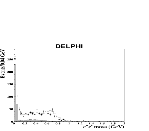
Refer to caption
Figure 6: Invariant mass $m_{{\rm e}^{+}{\rm e}^{-}}$ distributions for pairs of oppositely charged particles with one or both particles identified as electron candidates and where both tracks have hits in theΒ VD. Data are dots, the simulation is the line. The shaded area shows the contribution from $\pi^{0}\to\gamma{\rm e}^{+}{\rm e}^{-}$ decays. The region $m_{{\rm e}^{+}{\rm e}^{-}}>{\mathit{200}}$Β MeV is dominated by misidentified $\pi^{+}\pi^{-}$Β pairs.

Fig.Β 6 shows the invariant mass distribution for pairs of oppositely charged particles in $\tau$ decay hemispheres containing three charged particles, where one or both of the pair were tagged as an electron candidate and where both tracks had hits in the VD. The electron mass was assumed for both particles. The VD association requirement rejected most photon conversions, which occurred after the VD, while not affecting the signal of $\pi^{0}$ Dalitz decays, or of hadrons misidentified as electrons. The contribution from Dalitz decays peaks at low masses, below the $\pi^{0}$ mass. The tail from Dalitz decays in the region of masses around 200Β MeV to 600Β MeV arises from decays where only one of the electron or positron was identified and there were two possible combinations of oppositely charged particles. In such decays only half the possible combinations were due to the ${\rm e}^{+}{\rm e}^{-}$ pair. In these cases each combination has been given a weight of one half. The region of mass greater than 200Β MeV was dominated by $\pi^{+}\pi^{-}$ pairs where one of the pions was misidentified as an electron. This permitted a determination from the data of the probability to misidentify a 3-prong $\tau$ decay as a 1-prong decay containing a conversion candidate. The misidentification probability was estimated to be $(1.29\pm 0.09)\%$. The uncertainty was dominated by data statistics and contained a contribution from the VD association efficiency. From the ratio of data to simulation in the low mass spike it was estimated that the efficiency to reject a $\pi^{0}$ Dalitz decay in data was 0.90$\pm$0.07 times the efficiency obtained in simulation. The uncertainty included contributions from the error on the Particle Data Group best estimation of the $\pi^{0}\to\gamma{\rm e}^{+}{\rm e}^{-}$ branching ratioΒ [5], the uncertainty in the VD efficiency and the limited simulation statistics in addition to the statistical uncertainty. No correction was applied to the simulation and a relative uncertainty of 10% on the Dalitz rejection efficiency was taken.

Most $\delta$-rays were rejected by the requirement of VD hits on a track. Events in simulation containing a $\delta$-ray were reweighted with the radius dependent factors describing the ratio of material in terms of radiation lengths $X^{{}^{EM}}_{d}/X^{{}^{EM}}_{s}$ inΒ TableΒ 1. There is some ambiguity in the choice of this factor. The associated systematic uncertainties are discussed in SectionΒ 6.2.3.

5.3 Nuclear reinteractions

About 3% of hadrons reinteract inelastically with the material before the TPC gas volume, and produce typically up to 10 charged secondary particles. These reinteractions were reconstructed by an algorithm which was designed to find secondary reinteraction vertices using the tracks from outgoing charged particles produced in nuclear reinteractions.

The algorithm was robust with respect to the number of charged particles produced and to the position of the reinteraction with the DELPHI detector material. Only tracks which had impact parameters inconsistent with coming from the interaction region were considered. The algorithm iterated over all pairs of tracks, and attempted to fit a vertex in three dimensions if neither of the tracks had already been included in an earlier successfully fitted vertex. However, if one of the tracks had already been included in an earlier fitted vertex, an attempt was made to include the other track in that vertex. This was the main part of the algorithm permitting the reconstruction of vertices with an arbitrary number of outgoing charged particle tracks. In the rare case where both tracks had already been associated to different fitted vertices, an attempt was made to merge those two vertices, if their positions were compatible. In all cases a candidate reinteraction vertex had to pass a $\chi^{2}$ cut and all outgoing tracks had to have a first observed hit consistent with the particle originating from the reconstructed vertex. Candidate vertices with two outgoing tracks and kinematically compatible with the decay of a $K^{0}_{\!\mathrm{S}}$ or $\Lambda$ produced in the interaction region were not considered.

A search was then performed for the incoming particle which caused the interaction. Tracks which had been reconstructed in only the VD or the VD and ID were extrapolated to the candidate nuclear reinteraction vertex, and associated to the vertex if consistency was found. This prevented double counting of VD-ID tracks and reconstructed nuclear reinteractions. If there was no such track the momentum and charge of the incoming hadron were estimated from the sum over the outgoing particles associated to the vertex. For $\tau$ decays it is a good approximation to assume all such nuclear reinteraction vertices are caused by charged particles, as $K^{0}$ mesons are the only source of neutral hadrons producing nuclear reinteractions and are infrequently produced.

In simulation, the algorithm was (82.4$\pm$0.2)% efficient in 1-prong $\tau$ decays for incoming particle momenta above 1Β GeV/$c$, and (83.2$\pm$0.4)% efficient in 3-prong $\tau$ decays. The efficiency had little dependence on the $\tau$ decay multiplicity or on the charged secondary particle multiplicity in the nuclear reinteraction. The position of the reinteraction vertex was reconstructed with a precision of better than 1Β mm in three dimensions.

Refer to caption
Figure 7: Distribution in ${\rm e}^{+}{\rm e}^{-}\rightarrow\tau^{+}\tau^{-}$ events of reconstructed radius of the inelastic nuclear reinteractions. Data are dots, the line is simulation after applying correction factors.

In a similar manner as for the converted photons, the reconstructed and unreconstructed nuclear reinteractions were studied as a function of the reinteraction radius. The rates of reconstructed nuclear reinteractions were obtained from the $\tau^{+}\tau^{-}$ sample in data and simulation. The radial distribution of reconstructed hadronic reinteractions is shown in Fig.Β 7. Some localised discrepancies, more marked than in the case of the photon conversions, are visible in the detailed description of the ID trigger layers and TPC in the simulation. The flat tail for radii greater than 35Β cm is due to reinteractions in the TPC cathode plane atΒ πœ½β‰ˆπŸ—πŸŽβˆ˜πœ½superscript90\theta\approx 90^{\circ}.

The unreconstructed nuclear reinteractions were measured by studying the multiplicity distribution for charged particle tracks with impact parameters in the r-$\phi$ plane greater than 1.5Β cm in the hemisphere opposite a well reconstructed leptonic $\tau$ decay candidate. Simulation studies showed that this was dominated by $\tau$ decays with an unreconstructed nuclear reinteraction for multiplicities of four and greater. The $\tau$ decay hemispheres used to estimate this effect had to have no reconstructed nuclear reinteraction. This removed the risk of a false measurement arising from potential discrepancies in the charged particle multiplicity due to data/simulation differences in the track inclusion efficiency of the nuclear reinteraction reconstruction algorithm. The reinteraction radius was taken as the radius of the material surface lying immediately inside the first measured point on any of the charged particle tracks with a high impact parameter.

Radius Inelastic nuclear reinteractions
Lower Upper $A^{{}^{nucl}}_{{}_{rec}}$ $A^{{}^{nucl}}_{{}_{unrec}}$ $\epsilon^{{}^{nucl}}_{d}/\epsilon^{{}^{nucl}}_{s}$ $X^{{}^{nucl}}_{d}/X^{{}^{nucl}}_{s}$
0cm 22.0cm 0.91$\pm$ 0.08 1.01$\pm$ 0.02 0.95$\pm$ 0.05 0.96$\pm$ 0.04
22.0cm 28.5cm 0.93$\pm$ 0.04 1.36$\pm$ 0.15 0.96$\pm$ 0.13 0.97$\pm$ 0.04
28.5cm 50cm 0.86$\pm$ 0.03 1.00$\pm$ 0.03 0.98$\pm$ 0.03 0.87$\pm$ 0.03
0cm 50cm 0.89$\pm$ 0.02 1.01$\pm$ 0.02 0.98$\pm$ 0.02 0.91$\pm$ 0.02
Table 2: Factors used to correct simulated nuclear reinteractions for data/simulation discrepancies as a function of the radius of the reinteraction point. Column 5 shows the data/simulation ratio of reconstruction efficiency and column 6 the equivalent ratio for the material.

The measured correction factors $A^{{}^{nucl}}_{{}_{rec}}$ and $A^{{}^{nucl}}_{{}_{unrec}}$, analogous to the quantities $A^{{}^{conv}}_{{}_{rec}}$ and $A^{{}^{conv}}_{{}_{unrec}}$ for conversions, are given inΒ TableΒ 2, together with the data/simulation ratio of the efficiencies for reconstruction of inelastic nuclear reinteractions $\epsilon^{{}^{nucl}}_{d}/\epsilon^{{}^{nucl}}_{s}$ and the derived data/simulation ratio of material in terms of nuclear interaction lengths $X^{{}^{nucl}}_{d}/X^{{}^{nucl}}_{s}$. The region of the ID jet chamber gas volume, (13Β cm toΒ 22Β cm) has been included together with the region at lower radius as it has a very small number of nuclear interaction lengths, of orderΒ πŸπŸŽβˆ’πŸ’superscript10410^{-4}. These results indicate that for nuclear interactions the material at lower radii than the TPC gas volume is over-estimated by about 9% in the simulation program while the reconstruction efficiency is consistent in data and simulation. There is a significant difference in the estimated data/simulation material ratios for nuclear and electromagnetic interactions. This can be attributed to the complexity of the composite material structure together with the means by which each of these quantities is introduced in the simulation program, as well as to possible weaknesses in the modelling of the hadronic reinteractions in the simulation program. The same effects are observed in ${\rm e}^{+}{\rm e}^{-}\rightarrow{\rm q}\bar{\rm q}$ events. The uncertainty in the initial production rate of hadrons in $\tau$ decays is relatively small and does not give an important systematic uncertainty in the measurement of $A^{{}^{nucl}}_{{}_{rec}}$ and $A^{{}^{nucl}}_{{}_{unrec}}$.

As for the photon conversions, the nuclear reinteractions were studied for each year separately, particularly before and after the upgrade of the ID trigger layer in 1995.

Simulation studies indicate that the probability of reconstructing a fake nuclear reinteraction from $\tau$ decay secondary particles where none was present was $5\times 10^{-4}$ in 3-prong $\tau$ decays. However most such events were still classified as 3-prongs. The associated uncertainty was taken to be 100% of the size of the effect. The probability of reconstructing a fake nuclear reinteraction from a $K^{0}_{\!\mathrm{S}}$ decay was negligible.

The probability that a hadron produced in a $\tau$ decay would undergo an elastic nuclear reinteraction before the TPC sensitive volume was estimated from simulation to be (3.29$\pm$0.05)%. The typical signature of such an interaction was a charged particle track with a kink at the scattering point in the detector material. For large scatters the reconstruction algorithm would not reconstuct one but two tracks, one before and one after the scatter. This led typically to a signature of one VD-ID track and one TPC-OD track, and did not alter the observed track multiplicity in the TPC and OD.

5.4 Topology selection criteria

By judicious application of the VD hits requirement, and taking into account that the $\tau$ must decay into an odd number of charged particles, algorithms were constructed to minimise the sensitivity to the VD association efficiency and the knowledge of the material reinteractions; these are described below. In the following a β€œgood” track is defined as a charged particle track which has associated TPC or OD hits and is not identified as originating from a conversion or nuclear reinteraction in the detector material. For simplicity, the VD-ID track classification, in addition to including tracks reconstructed using only the VD and ID detectors, includes tracks reconstructed as the ingoing charged hadron to a nuclear reinteraction. In $\tau$ decay hemispheres where the presence of a converted photon was signalled by the electron identification algorithm, the observed number of good tracks was reduced by two (or by one in the rare case of an even number of good tracks) for the purposes of the topology classification.

Individual $\tau$ decay hemispheres were allotted to five different classes dependent on the number of reconstructed tracks in the TPC, VD, etc. The first three of these classes correspond closely to events with clean reconstruction of a 1-prong, 3-prong or 5-prong topology. The other two classes contain the small number of $\tau$ decay hemispheres where there was more ambiguity in the reconstruction of the topology, but where some discrimination was still possible.

A 1-prong $\tau$ decay was defined as a $\tau$ decay hemisphere satisfying any of the following criteria:

  • β€’

    only one good track with associated VD hits, and no other tracks with associated VD hits;

  • β€’

    only one good track, without VD or ID hits, and one VD-ID track;

  • β€’

    no good tracks, and only one VD-ID track.

3-prong $\tau$ decays were isolated by demanding $\tau$ decay hemispheres satisfying at least one of the following sets of criteria:

  • β€’

    three, four or five good tracks, of which either two or three had VD hits;

  • β€’

    two good tracks with associated VD hits, plus one VD-ID track;

  • β€’

    one good track with associated VD hits, plus one or two VD-ID tracks pointing within $3^{\circ}$ in azimuth of a TPC sector boundary.

Candidate 5-prong $\tau$ decays were selected if they satisfied at least one of the following topological criteria:

  • β€’

    five good tracks of which at least four had two or more associated VD hits;

  • β€’

    four good tracks with VD hits, and one other VD-ID track.

Additional criteria were applied in the selection of 5-prong $\tau$ decays due to the large potential background from hadronic $Z$ decays and mis-reconstructed 3-prong $\tau$ decays. The background originating from $\nu_{\tau}3h^{\pm}\geq 1\pi^{0}$ final states with a Dalitz decay was expected to occur at a similar level to the signal. The electron rejection criteria described in SectionΒ 5.2 reduced this background by about 70%, and it was further suppressed by requiring that all good tracks had a momentum greater thanΒ 1Β GeV/$c$. To reject $Z\to{\rm q}\bar{\rm q}$ events it was required that the total momentum of the 5-prong system be greater than 20Β GeV/$c$. Only good tracks were included in the calculation of this quantity.

These three classes accounted for 97.6% of candidate $\tau$ decays in the $\tau^{+}\tau^{-}$ sample. The remaining 2.4% of candidate $\tau$ decays were mostly 1-prong and 3-prong $\tau$ decays with some pattern recognition failure or detector inefficiency. These were classified into two categories, $1^{\prime}$ and $3^{\prime}$, corresponding to 1-prong and 3-prong $\tau$ decays respectively. Candidate $\tau$ decay hemispheres of type $1^{\prime}$ had to satisfy at least one of the following criteria:

  • β€’

    one good track, with associated VD hits, plus two VD-ID tracks not pointing within $3^{\circ}$ in azimuth of a TPC sector boundary;

  • β€’

    one good track, plus a conversion candidate selected with the electron identification algorithm.

The $3^{\prime}$ category contained all other $\tau$ decay hemispheres failing to pass any of the previous classification requirements. In particular it contained those events with either four or five good tracks of which either four or more had associated VD hits, but not satisfying the 5-prong class requirements. This criteria had a higher efficiency for 5-prong decays than for 3-prong decays, but due to the much greater 3-prong branching ratio the $3^{\prime}$ category was dominated by 3-prong decays. TableΒ 3 contains the efficiencies of these selection requirements for the different exclusive $\tau$ decay modes and the inclusive single-hemisphere topological selections, as obtained from simulation and after corrections for observed discrepancies between data and simulation in the rate and reconstruction efficiency of material reinteractions.

true $\tau$ $\tau^{+}\tau^{-}$ Topology Classification
decay mode selection 1 3 5 $1^{\prime}$ $3^{\prime}$
$\rm e^{-}\bar{\nu_{\rm e}}\nu_{\tau}$ 50.60$\pm$ 0.07 99.95$\pm$ 0.00 0.00$\pm$ 0.00 0.00$\pm$ 0.00 0.02$\pm$ 0.00 0.02$\pm$ 0.00
$\mu^{-}\bar{\nu_{\tau}}\nu_{\mu}$ 53.31$\pm$ 0.07 99.96$\pm$ 0.00 0.00$\pm$ 0.00 0.00$\pm$ 0.00 0.01$\pm$ 0.00 0.03$\pm$ 0.00
$\pi^{-}\nu_{\tau}$ 49.69$\pm$ 0.09 99.88$\pm$ 0.01 0.04$\pm$ 0.01 0.00$\pm$ 0.00 0.00$\pm$ 0.00 0.08$\pm$ 0.01
$\pi^{-}\pi^{0}\nu_{\tau}$ 51.77$\pm$ 0.06 97.87$\pm$ 0.03 0.60$\pm$ 0.01 0.00$\pm$ 0.00 0.84$\pm$ 0.02 0.69$\pm$ 0.01
$\pi^{-}2\pi^{0}\nu_{\tau}$ 51.07$\pm$ 0.11 95.88$\pm$ 0.06 1.25$\pm$ 0.03 0.00$\pm$ 0.00 1.42$\pm$ 0.04 1.45$\pm$ 0.04
$\pi^{-}3\pi^{0}\nu_{\tau}$ 48.89$\pm$ 0.25 94.36$\pm$ 0.16 1.68$\pm$ 0.09 0.00$\pm$ 0.00 1.83$\pm$ 0.10 2.13$\pm$ 0.10
$K^{-}\nu_{\tau}$ 49.43$\pm$ 0.36 99.90$\pm$ 0.03 0.02$\pm$ 0.02 0.00$\pm$ 0.00 0.01$\pm$ 0.01 0.06$\pm$ 0.03
$K^{-}\pi^{0}\nu_{\tau}$ 51.40$\pm$ 0.47 97.66$\pm$ 0.20 0.85$\pm$ 0.12 0.00$\pm$ 0.00 0.80$\pm$ 0.12 0.69$\pm$ 0.11
$K^{-}2\pi^{0}\nu_{\tau}$ 50.42$\pm$ 1.12 94.65$\pm$ 0.71 2.28$\pm$ 0.47 0.00$\pm$ 0.00 1.39$\pm$ 0.37 1.68$\pm$ 0.40
$\pi^{-}K^{0}_{\!\mathrm{L}}\nu_{\tau}$ 53.10$\pm$ 0.48 99.79$\pm$ 0.06 0.07$\pm$ 0.03 0.00$\pm$ 0.00 0.00$\pm$ 0.00 0.14$\pm$ 0.05
$\pi^{-}K^{0}_{\!\mathrm{L}}\pi^{0}\nu_{\tau}$ 51.85$\pm$ 0.73 97.32$\pm$ 0.33 0.78$\pm$ 0.18 0.00$\pm$ 0.00 0.78$\pm$ 0.18 1.11$\pm$ 0.21
$K^{-}K^{0}_{\!\mathrm{L}}\nu_{\tau}$ 54.60$\pm$ 0.87 99.78$\pm$ 0.11 0.11$\pm$ 0.08 0.00$\pm$ 0.00 0.00$\pm$ 0.00 0.11$\pm$ 0.08
$K^{-}K^{0}_{\!\mathrm{L}}\pi^{0}\nu_{\tau}$ 52.66$\pm$ 1.24 96.71$\pm$ 0.61 0.94$\pm$ 0.33 0.00$\pm$ 0.00 0.94$\pm$ 0.33 1.41$\pm$ 0.40
$\pi^{-}K^{0}_{\!\mathrm{L}}K^{0}\nu_{\tau}$ 52.82$\pm$ 1.04 95.12$\pm$ 0.62 3.72$\pm$ 0.54 0.00$\pm$ 0.00 0.08$\pm$ 0.08 1.07$\pm$ 0.30
$\pi^{-}K^{0}_{\!\mathrm{S}}\nu_{\tau}$ 52.17$\pm$ 0.48 94.48$\pm$ 0.30 4.30$\pm$ 0.27 0.00$\pm$ 0.00 0.16$\pm$ 0.05 1.06$\pm$ 0.14
$\pi^{-}K^{0}_{\!\mathrm{S}}\pi^{0}\nu_{\tau}$ 50.78$\pm$ 0.73 92.64$\pm$ 0.54 4.65$\pm$ 0.43 0.00$\pm$ 0.00 0.55$\pm$ 0.15 2.16$\pm$ 0.30
$K^{-}K^{0}_{\!\mathrm{S}}\nu_{\tau}$ 52.38$\pm$ 0.86 94.50$\pm$ 0.54 4.42$\pm$ 0.49 0.00$\pm$ 0.00 0.06$\pm$ 0.06 1.02$\pm$ 0.24
$K^{-}K^{0}_{\!\mathrm{S}}\pi^{0}\nu_{\tau}$ 51.32$\pm$ 1.32 92.56$\pm$ 0.97 5.01$\pm$ 0.80 0.00$\pm$ 0.00 0.41$\pm$ 0.23 2.03$\pm$ 0.52
$\pi^{-}2K^{0}_{\!\mathrm{S}}\nu_{\tau}$ 46.34$\pm$ 1.80 86.72$\pm$ 1.80 10.45$\pm$ 1.63 0.00$\pm$ 0.00 0.00$\pm$ 0.00 2.82$\pm$ 0.88
1-prong 51.42$\pm$ 0.03 98.71$\pm$ 0.01 0.42$\pm$ 0.01 0.00$\pm$ 0.00 0.44$\pm$ 0.01 0.43$\pm$ 0.01
$2\pi^{-}\pi^{+}\nu_{\tau}$ 54.71$\pm$ 0.11 0.90$\pm$ 0.03 90.26$\pm$ 0.09 0.01$\pm$ 0.00 2.10$\pm$ 0.04 6.74$\pm$ 0.07
$2\pi^{-}\pi^{+}\pi^{0}\nu_{\tau}$ 53.88$\pm$ 0.13 1.26$\pm$ 0.04 86.39$\pm$ 0.12 0.10$\pm$ 0.01 3.15$\pm$ 0.06 9.10$\pm$ 0.10
$3\pi^{\pm}2\pi^{0}\nu_{\tau}$ 53.14$\pm$ 0.46 1.37$\pm$ 0.15 83.64$\pm$ 0.46 0.22$\pm$ 0.06 3.68$\pm$ 0.24 11.09$\pm$ 0.39
$3\pi^{\pm}3\pi^{0}\nu_{\tau}$ 52.13$\pm$ 1.06 1.46$\pm$ 0.35 78.73$\pm$ 1.20 0.17$\pm$ 0.12 4.74$\pm$ 0.62 14.90$\pm$ 1.05
$K^{-}\pi^{-}\pi^{+}\nu_{\tau}$ 54.64$\pm$ 0.56 1.03$\pm$ 0.15 90.35$\pm$ 0.45 0.00$\pm$ 0.00 1.70$\pm$ 0.20 6.92$\pm$ 0.38
$K^{-}K^{+}\pi^{+}\nu_{\tau}$ 53.87$\pm$ 0.90 2.08$\pm$ 0.35 87.23$\pm$ 0.82 0.00$\pm$ 0.00 1.10$\pm$ 0.26 9.59$\pm$ 0.73
3-prong 54.32$\pm$ 0.08 1.06$\pm$ 0.02 88.51$\pm$ 0.07 0.05$\pm$ 0.00 2.54$\pm$ 0.03 7.84$\pm$ 0.06
$3\pi^{-}2\pi^{+}\nu_{\tau}$ 49.63$\pm$ 1.19 0.11$\pm$ 0.11 12.63$\pm$ 1.13 57.52$\pm$ 1.67 0.23$\pm$ 0.16 29.51$\pm$ 1.55
$5\pi^{\pm}\pi^{0}\nu_{\tau}$ 48.91$\pm$ 2.23 0.00$\pm$ 0.00 15.04$\pm$ 2.28 52.85$\pm$ 3.18 0.81$\pm$ 0.57 31.30$\pm$ 2.96
5-prong 49.47$\pm$ 1.05 0.09$\pm$ 0.09 13.16$\pm$ 1.01 56.49$\pm$ 1.48 0.36$\pm$ 0.18 29.90$\pm$ 1.37
Table 3: Estimates of the selection and topology classification efficiencies, in percent, for different exclusive decay modes, as obtained from simulation. The efficiencies are corrected for observed discrepancies between data and simulation in the rate and reconstruction efficiency of material reinteractions. The quoted uncertainties are from the simulation statistics only.

Events were classified according to both the hemisphere classifications into 14 event topology classes: 1-1, 1-$1^{\prime}$, 1-3, 1-$3^{\prime}$, 1-5, $1^{\prime}$-$1^{\prime}$, $1^{\prime}$-3, $1^{\prime}$-$3^{\prime}$, $1^{\prime}$-5, 3-3, 3-$3^{\prime}$, 3-5, $3^{\prime}$-$3^{\prime}$ and $3^{\prime}$-5. The class 5-5 was not included as these events were removed by the multiplicity cut in the $\tau^{+}\tau^{-}$ preselection and in any case would give a negligible signal contribution. The selection of event classes up to multiplicity five assumes that the inclusive branching ratio of the $\tau$ to seven charged particles is negligible. While inclusion of higher multiplicity classes is possible, the DELPHI sample size is insufficient to reach the level of precision obtained by CLEOΒ [16].

The various sources of non-$\tau^{+}\tau^{-}$ background are detailed in TableΒ 4 for each of the event topology classes.

Source of All Event Topology
Background Topologies 1-1 1-$1^{\prime}$ 1-3 1-$3^{\prime}$ 1-5 $1^{\prime}$-$1^{\prime}$ $1^{\prime}$-3 $1^{\prime}$-$3^{\prime}$ $1^{\prime}$-5 3-3 3-$3^{\prime}$ 3-5 $3^{\prime}$-$3^{\prime}$ $3^{\prime}$-5
$\mu^{+}\mu^{-}$ 0.11 $\pm$ 0.01 0.19 0.06 0.00 0.07 0.00 0.00 0.00 0.00 0.00 0.00 0.00 0.00 0.00 0.00
${\rm e}^{+}{\rm e}^{-}$ 0.40 $\pm$ 0.07 0.65 0.00 0.01 0.00 0.00 0.00 0.00 0.00 0.00 0.00 0.00 0.00 0.00 0.00
${\rm q}\bar{\rm q}$ 0.29 $\pm$ 0.01 0.03 0.00 0.32 3.39 1.01 0.00 1.16 0.00 0.00 1.61 14.8 21.2 77.0 0.00
${\rm e}^{+}{\rm e}^{-}{\rm e}^{+}{\rm e}^{-}$ 0.27 $\pm$ 0.03 0.49 0.00 0.00 0.00 0.00 0.00 0.00 0.00 0.00 0.00 0.00 0.00 0.00 0.00
${\rm e}^{+}{\rm e}^{-}\mu^{+}\mu^{-}$ 0.10 $\pm$ 0.01 0.16 0.00 0.01 0.00 0.00 0.00 0.00 0.00 0.00 0.00 0.33 0.00 0.00 0.00
${\rm e}^{+}{\rm e}^{-}\tau^{+}\tau^{-}$ 0.27 $\pm$ 0.03 0.35 3.91 0.23 0.76 0.00 21.1 0.97 2.88 0.00 0.20 0.60 0.00 0.45 0.00
${\rm e}^{+}{\rm e}^{-}{\rm q}\bar{\rm q}$ 0.02 $\pm$ 0.01 0.03 0.00 0.03 0.44 0.00 0.00 0.00 0.00 0.00 0.00 0.00 0.00 0.00 0.00
cosmic rays 0.05 $\pm$ 0.01 0.07 0.01 0.00 0.00 0.00 0.00 0.00 0.00 0.00 0.00 0.00 0.00 0.00 0.00
Total 1.51 $\pm$ 0.10 1.97 3.98 0.60 4.66 1.01 21.1 2.13 2.88 0.00 1.81 15.7 21.2 77.4 0.00
Table 4: Fractional non-$\tau^{+}\tau^{-}$ backgrounds (in %) in the $\tau^{+}\tau^{-}$ sample and the different event topology classes. The classes 1${}^{~{}\!\!\prime}$-5 and 3${}^{~{}\!\!\prime}$-5 have very small populations and the estimated background is zero due to statistical fluctuations in the simulation.

6 The fit and systematics

6.1 Fitting procedure

A reweighting technique was used to take into account the observed data/simulation discrepancies in the rates and reconstruction efficiencies of nuclear reinteractions, photon conversions and $\delta$-rays. Each secondary or tertiary particle $i$ in a simulated $\tau^{+}\tau^{-}$ eventΒ π’Œπ’Œk was given a weightΒ π‘Ύπ’Šπ’‘β€‹π’‚β€‹π’“β€‹π’•subscriptsuperscriptπ‘Ύπ’‘π’‚π’“π’•π’ŠW^{part}_{i}. For particles interacting with the detector material this weight was obtained from the studies described in SectionΒ 5 and summarised in TablesΒ 1 andΒ 2. These weights were a function of the radius and type of the reinteraction, as follows:

  • β€’

    reconstructed converted photons: $W^{part}_{i}=A^{{}^{conv}}_{{}_{rec}}({\mathrm{r}})$;

  • β€’

    unreconstructed converted photons: $W^{part}_{i}=A^{{}^{conv}}_{{}_{unrec}}({\mathrm{r}})$;

  • β€’

    reconstructed inelastic nuclear reinteractions: $W^{part}_{i}=A^{{}^{nucl}}_{{}_{rec}}({\mathrm{r}})$;

  • β€’

    unreconstructed inelastic nuclear reinteractions: $W^{part}_{i}=A^{{}^{nucl}}_{{}_{unrec}}({\mathrm{r}})$;

  • β€’

    𝜹𝜹\delta-rays: $W^{part}_{i}=X^{{}^{EM}}_{d}/X^{{}^{EM}}_{s}({\mathrm{r}})$;

  • β€’

    bremsstrahlung emitting electrons: $W^{part}_{i}=X^{{}^{EM}}_{d}/X^{{}^{EM}}_{s}({\mathrm{r}})$;

  • β€’

    elastic nuclear reinteractions: $W^{part}_{i}=X^{{}^{nucl}}_{d}/X^{{}^{nucl}}_{s}({\mathrm{r}})$.

It was also necessary to reweight particles which did not reinteract so as to maintain the internal normalisation of the simulation sample with respect to parameters such as angular distributions, momentum distributions, or the $\tau$ exclusive branching ratios. Failure to achieve this could lead to biases within the simulation sample as a function of photon multiplicities, charged hadron multiplicities, angular regions with different amounts of material, or could bias the preselection of the $\tau^{+}\tau^{-}$ sample with respect to certain types of decay mode. Non-interacting photons were given a weightΒ π‘Ύπ’Šπ’‘β€‹π’‚β€‹π’“β€‹π’•subscriptsuperscriptπ‘Ύπ’‘π’‚π’“π’•π’ŠW^{part}_{i}Β givenΒ by

$$W^{part}_{i}=\frac{N^{{}^{\gamma}}-\!\!\!\!\displaystyle\sum_{j\in\mathrm{int.photons}}\!\!\!\!\!\!\!\!W^{part}_{j}}{N^{{}^{\gamma}}-N^{\gamma}_{int}},$$ (8)

where $N^{\gamma}$ is the total number of photons produced by $\tau$ decays or by interactions with material of $\tau$ decay products in the simulation sample. $N^{\gamma}_{int}$ is the number of photons with a material reinteraction. The sum is over all photons with a material reinteraction. To maintain the angular and momentum distributions the above weight calculation was performed separately for individual bins in a three-dimensional space of the photon polar angle, azimuthal angle and momentum. A similar procedure was used to reweight non-interacting hadrons, particles not emitting a $\delta$-ray (a very small correction) and electrons without any bremsstrahlung emission.

With every secondary and tertiary particle $i$ in a simulated event $k$ given a weight $W^{part}_{i}$, the weight $W^{event}_{k}$ of the event was given by the product of all these weights:

$$W^{event}_{k}=\prod_{i\in k}W^{part}_{i}.$$ (9)

The numbers of selected events in each event topology class are shown in TableΒ 5. A maximum likelihood fit assuming Poissonian probabilities was performed to the reweighted numbers of events estimated using Eqn.Β 3. The number of $\tau^{+}\tau^{-}$ events ($N_{\tau\tau}$ in Eqn.Β 3) and the branching ratios $B_{1}$ and $B_{5}$ were allowed to vary in the fit while $B_{3}$ was constrained by the relation $B_{1}+B_{3}+B_{5}=1$. The output of the fit is also shown in TableΒ 5. The results of this fit were: $B_{1}=(85.316\pm 0.093)\%$; $B_{3}=(14.569\pm 0.093)\%$; $B_{5}=(0.115\pm 0.013)\%$, where only the statistical error from the fit is quoted. An estimate of the consistency of the fit was made by calculating a $\chi^{2}$. This took into account only the statistical uncertainties. It gave a $\chi^{2}/$n.d.f. of $16.4/11$, indicating good consistency. The contribution to the $\chi^{2}$ from each class is shown in TableΒ 5.

Class Observed Fit Output $\chi^{2}$
1 $-$ 1 56219 56149.0 0.1
1 $-$ $1^{\prime}$ 858 871.0 0.2
1 $-$ 3 18681 18813.5 0.9
1 $-$ $3^{\prime}$ 2350 2331.5 0.1
1 $-$ 5 94 95.6 0.0
$1^{\prime}$ $-$ $1^{\prime}$ 4 3.9 0.0
$1^{\prime}$ $-$ 3 131 134.8 0.1
$1^{\prime}$ $-$ $3^{\prime}$ 16 14.7 0.1
$1^{\prime}$ $-$ 5 0 1.2 1.2
3 $-$ 3 1481 1451.5 0.6
3 $-$ $3^{\prime}$ 409 357.4 7.4
3 $-$ 5 17 13.8 0.7
$3^{\prime}$ $-$ $3^{\prime}$ 76 97.7 4.8
$3^{\prime}$ $-$ 5 1 1.5 0.2
All 80337 80337.1 16.4
Table 5: The second and third columns contain the number of observed events in each class and number predicted from the maximum likelihood fit of the $\tau$ topological branching ratios. The fourth column contains the $\chi^{2}$ contribution for each class to the overall $\chi^{2}$.

6.2 Systematics

In general, the systematic uncertainties on the topological branching ratios due to any particular effect were estimated simultaneously for $B_{1}$, $B_{3}$ and $B_{5}$ by repeating the analysis, including the $\tau^{+}\tau^{-}$ preselection, after modifying the relevant variable in the simulation. This accounted for correlations in the systematic uncertainties between the different branching ratios and correlations in efficiencies and backgrounds between the different event classes and the $\tau^{+}\tau^{-}$ preselection.

6.2.1 Preselection

The main systematic effects of the $\tau^{+}\tau^{-}$ selection criteria on the result can arise through the mis-calibration of the quantities used in the selection. These quantities can be classified into cuts related to energy or momentum measurements, such as $E_{rad}$, $p_{rad}$ and $E_{vis}$, or those cuts related to multiplicity, such as the isolation angle, which can be incorrectly estimated if extra secondary particles are produced in reinteractions with detector material. This second effect is taken account of by the systematics in the reweighting of the secondary interactions, discussed in SectionΒ 6.2.3. A separate systematic uncertainty is included for the energy and momentum scales below. Other effects such as tracking efficiency, trigger efficiency and uncertainties on the $\tau$ exclusive branching ratios can have an effect on the $\tau^{+}\tau^{-}$ preselection efficiency. These sources of systematic uncertainty are discussed below, and in general the systematic uncertainties on the topological branching ratios take into account effects in the preselection.

Any remnant discrepancies due to $\tau^{+}\tau^{-}$ preselection criteria were checked by studying the agreement between data and simulation for the distributions of the $\tau^{+}\tau^{-}$ selection variable for each of the different event topology classes. With the corrections to the background levels discussed in SectionsΒ 4.2 andΒ 5, good agreement was found, in particular in the regions of the cuts.

The uncertainties due to the backgrounds from non-$\tau^{+}\tau^{-}$ sources were estimated by varying the background normalisations by their uncertainties obtained as described in SectionΒ 4, and are listed in TableΒ 6. The distribution of the neural network variable used for ${\rm q}\bar{\rm q}$ rejection (see Fig.Β 2) displays a 15% excess in the data compared with simulation in the region [0.05;0.8] of the output neuron distribution. This region was dominated by $\tau^{+}\tau^{-}$ events and was studied to see if there were any discrepancies in the input variables, and by checking the multiplicity distributions of the events. No discrepancies were found. The systematic uncertainty was estimated by rescaling the numbers of rejected signal events in all classes byΒ 15%.

6.2.2 Tracking

Within the angular acceptance of this analysis, there are four tracking detectors which can contribute to the track reconstruction of all charged particles: the VD, ID, TPC and OD. The reconstruction of β€œgood” tracks is strongly dependent on the TPC with its full three-dimensional readout. The redundancy in the track reconstruction obtained by the inclusion of $\tau$ decay hemispheres with only a VD-ID track in the $\tau^{+}\tau^{-}$ sample and 1-prong subsample reduces greatly the sensitivity of the measurement to inefficiencies within a given subdetector, and allows direct cross-checks to be made.

In simulation, for non-interacting particles, the efficiency for the TPC to reconstruct an isolated charged particle which passes through a sensitive gas volume far from dead regions is 99.95%. However, even with the redundancy of the different tracking subdetector components in DELPHI, to measure this in data directly is difficult because of material reinteractions between different subdetectors which can cause the particle to be lost before entering the TPC sensitive volume. These effects tend to reduce the measured efficiency. For the data, the efficiency of the TPC in its sensitive regions was estimated using the redundancy of the tracking system to be $(99.35\pm 0.05)\%$. The identical procedure was applied to the simulation, yielding an efficiency of $(99.31\pm 0.01)\%$, in excellent agreement with the data, and implying that the modelling of the TPC efficiency in the simulation was accurate. The true inefficiency in simulation is a factor of 12 lower than the inefficiency estimated by this method. The uncertainty on the TPC reconstruction efficiency in the TPC sensitive region was taken conservatively to be $0.05\%$ to account for any systematic effects in its estimation.

The TPC efficiency for isolated tracks in the sector boundary region was studied using inclusive low multiplicity events but excluding the $\tau^{+}\tau^{-}$ events. This sample consists of radiative dilepton events and the high energy part of the two-photon leptonic event spectrum. The number of reconstructed tracks in the TPC boundary region was compared to that expected by normalisation of the sensitive region of the TPC sectors, in bins of momentum. The loss of tracks was compatible with zero below about 5Β GeV/$c$, rising to 3.5% at 45Β GeV/$c$. Data and simulation agree well in their behaviour. The inefficiency estimated from data for the $\tau^{+}\tau^{-}$ momentum distribution was $(2.73\pm 0.04)\%$, compatible with the result in simulated $\tau^{+}\tau^{-}$ events. The TPC efficiency was varied by throwing away tracks containing TPC hits in simulation and repeating the analysis, including the $\tau^{+}\tau^{-}$ preselection stage. The error was scaled by a factor two to account for any systematic effects in the procedure.

The attachment of VD hits to a track is the main criterion used in this analysis to determine the multiplicity of a $\tau$ decay. The association efficiency and mis-association probability of a VD hit to be attached to a charged particle track has been studiedΒ [20] on large samples of ${\rm e}^{+}{\rm e}^{-}\rightarrow{\rm q}\bar{\rm q}$ events, and on isolated topologies such as $\mu^{+}\mu^{-}$ final states. These studies indicate that the efficiency in simulation and data agree to within $\pm 2\%$. The associated systematic uncertainties were obtained from the shifts in the results observed when randomly removing 2% of associated VD hits and repeating the analysis, including the $\tau^{+}\tau^{-}$ preselection stage.

Within the $\tau$ sample itself the rate of association of different subdetectors to a reconstructed charged particle track was studied for different $\tau$ decay topologies. In candidate 1-prong decays, the hit association probabilities for the VD, ID and OD were studied for tracks which had an associated TPC track segment. The probabilities obtained in data and simulation were compared and the relative differences calculated. These differences were 0.0% for the VD, +2.3% for the ID and $-$1.2% for the OD. The equivalent numbers for 3-prong decays were $-$0.7%, +2.5% and +0.6% respectively. The results for the ID were unchanged if in addition the VD was required to be associated to a track, and vice-versa. The small fraction of tracks without a TPC track segment showed a level of agreement for the proportions of tracks with different subdetectors which was better than 3% in all cases.

In simulation, the preselection efficiency was found to be independent of the combination of the subdetectors attached to a track at a level belowΒ 0.1%. Given the observed discrepancies between data and simulation, any effect on the preselection efficiency due to this source wasΒ π“žβ€‹(πŸπŸŽβˆ’πŸ“)π“žsuperscript105{\cal{O}}(10^{-5}). The uncertainties arising from the probability of including an ID hit on a track were estimated to be $2.2\times 10^{-5}$ for both $B_{1}$ and $B_{3}$ with a full anticorrelation and has been included in the tracking systematic uncertainty. The analogous uncertainty for the OD was negligible.

It was observed that the level of Bhabha background was correlated with the existence of an OD hit on a track. This was due to bremsstrahlung, and resolution effects in the $p_{rad}$ variable. The level of agreement observed between the data and the simulation implied that the Bhabha background was consistent with the estimation made in SectionΒ 4.2.

Refer to caption

aRefer to captionb

Figure 8: a) The selection efficiency in simulation for candidate 3-prong decays as a function of the minimum angle in three dimensions between any two charged particles. b)Β TheΒ distribution of the minimum angle in three dimensions between any two charged particles in candidate 3-prong $\tau$ decays. Dots are data, line is simulation.
Refer to caption
Figure 9: The minimum angle in three dimensions between any two charged particles in candidate 5-prong $\tau$ decays. Dots are data, line is simulation.

The two-track resolution has been studied by data-simulation comparison of the minimum opening angle in three dimensions between tracks in $\tau$ decay hemispheres with more than one track. Fig.Β 8a shows the efficiency in simulation to reconstruct a 3-prong $\tau$ decay as a function of the minimum opening angle. It is flat within 1% except for a fall-off of about 5% in reconstruction efficiency for a minimum opening angle below 3Β mrad. As is visible in the distribution of the minimum opening angle in candidate 3-prong $\tau$ decays shown in Fig.Β 8b, less than 1% of 3-prong $\tau$ decays lie in this region and data and simulation are compatible within the statistical precision. A systematic uncertainty was attributed to the two-track resolution by varying the efficiency in the region with minimum opening angle below 3Β mrad by the uncertainty allowed from the statistical uncertainty of the data. There was no observable fall-off in efficiency for low values of the minimum differences between the azimuthal or polar angles of tracks in a 3-prong hemisphere. The minimum opening angle distribution in candidate 5-prong $\tau$ decays is shown inΒ Fig.Β 9.

Refer to caption
Figure 10: For candidate 3-prong $\tau$-decays, the ratio of data to simulation of the fraction of candidate decays where three tracks had associated TPC hits, as a function of the minimum opening angle.

The association efficiency of the TPC in 3-prong $\tau$ decays and its dependence on the minimum opening angle were studied by comparing the rate of candidate $\tau$ decays containing three tracks with associated TPC hits with the rate of decays containing either two tracks with TPC hits plus one track without TPC hits or one track with TPC hits plus two tracks without TPC hits. Fig.Β 10 shows the data over simulation ratio of the fraction of candidate 3-prong $\tau$ decays containing three tracks with associated TPC hits, as a function of the minimum opening angle. It shows compatibility with unity in all regions except for a small discrepancy of about +3% for minimum opening angles in the region of 4 to 7 mrad. The average of the ratio for all minimum opening angles is $1.0016\pm 0.0008$, consistent with unity within two standard deviations. The difference from unity can be directly related to the efficiency for a charged particle track to have associated TPC hits in 3-prong $\tau$ decays. The uncertainties on the topological branching ratios were estimated by varying the probability in simulated 3-prong $\tau$ decays to have TPC hits associated to a track by $1.6\times 10^{-3}$ and repeating the analysis. The same procedure was carried out for 5-prong decays.

Fig.Β 8b shows some differences between data and simulation in the region betweenΒ 3 and 15Β mrad, with the simulation tending to lie slightly above the data. This can be due to the decay modelling, for which the attendant systematic uncertainties are discussed in SectionΒ 6.2.4. However track reconstruction effects cannot be excluded. While systematics in the TPC association efficiency are accounted for above, the deviation from unity of the ratio shown in FigΒ 10 can also give an estimate of the rate of track reconstruction without the TPC, in particular of VD-ID tracks. An upper estimate of the magnitude of this effect for close tracks was derived by integrating up to 15Β mrad the deviations from unity of this ratio times the number of events in a given bin of minimum opening angle. This procedure gave an uncertainty of $1.2\times 10^{-4}$ on $B_{3}$, together with uncertainties on $B_{1}$ and $B_{5}$ induced via the correlations in the fit. This accounted for potential differences between data and simulation in the VD-ID track reconstruction in the small minimum opening angle region of 3-prong $\tau$ decays.

The reconstructed charge in a $\tau$ decay hemisphere was studied for different event and decay topologies. The charge was not used to classify $\tau$ decays or select $\tau^{+}\tau^{-}$ events, so this provided an indirect cross-check of the track reconstruction. Use was made of the constraint that the two $\tau$-decay hemispheres arose from $\tau$’s of opposite charge. For events in the data belonging to the 1-1 event class, an estimated (99.88$\pm$0.01)% of $\tau$ decays had the charge correctly reconstructed. The rate in the simulation was (99.91$\pm$0.01)%. For 3-prong decays in data, (98.57$\pm$0.09)% had the correctly signed unit charge, compared with (98.60$\pm$0.03)% in simulation, while (0.54$\pm$0.06)% had a charge of three with the correct sign as compared with (0.52$\pm$0.02)% in simulation. The remainder had the wrongly signed charge. In 5-prong decays an estimated (90.5$\pm$0.7)% had the correctly reconstructed unit charge in data compared with (89.7$\pm$0.3)% in simulation.

6.2.3 Reinteractions and $K^{0}_{\!\mathrm{S}}$ reconstruction

Uncertainties from the photon conversion reconstruction were estimated by varying by their uncertainties the correction factors for the reconstructed and unreconstructed conversions, given in TableΒ 1, which were obtained from data test samples as described in SectionΒ 5.2. A contribution for the uncertainty in the incident photon rate in the dileptonic test samples was included. The resultant uncertainties are dominated by the contribution from the unreconstructed conversions. A similar approach was taken for the nuclear reinteractions. Here again the uncertainty arising from the unreconstructed nuclear reinteractions was the most significant contribution.

Both the photon conversion and hadronic reinteraction errors contain contributions to account for the uncertainty on the rate of fake reconstructions which cause the topology to be misidentified.

The 1-prong $\tau$ decay class has a number of different subclasses which cover the different reconstruction possibilities for an elastic nuclear reinteraction in a 1-prong hadronic $\tau$ decay. In simulation, of the 3.3% of hadrons in $\tau$ decays undergoing an elastic scatter before the TPC sensitive volume 99.4% were correctly attributed to the 1-prong class, leading to a classification inefficiency of $2.0\times 10^{-4}$ for 1-prong hadronic $\tau$ decays. A cross-check of the elastic scatters was performed using a kink algorithm which attempted to link up pairs of tracks consistent with both tracks having been produced by a single charged particle experiencing a large scatter in detector material. Comparison of the rates in data and simulation showed agreement within 20%, which was taken as a relative uncertainty on the effect. The effects of fake kink reconstructions by the algorithm had a negligible effect.

The uncertainty attributed to the electron identification had contributions from the uncertainties on the efficiencies for conversion rejection and for rejection of $\pi^{0}$ Dalitz decays, and from the probability of misidentifying a hadron as an electron. The study of the electron identification algorithm and its systematic uncertainties is described in SectionΒ 5.2.

The $\delta$-ray rate is proportional to the mean atomic number Z of the material, while the factors which are applied correct for the number of radiation lengths, which is approximately proportional to the mean Z2. This gives an ambiguity in the correction for $\delta$-rays depending on whether it is due to the wrong mean Z, or to the wrong quantity of material, but with the correct mean Z. The correction factor used in the analysis, $X^{EM}_{d}/X^{EM}_{s}$, assumes the latter case. The former case would imply a factor of $(X^{EM}_{d}/X^{EM}_{s})^{1/2}$. This was applied and the observed variations on the branching ratios taken as systematic uncertainties.

Only the fraction ($\approx$5%) of $K^{0}_{\!\mathrm{S}}\to\pi^{+}\pi^{-}$ decays occuring inside the VD, and which the $K^{0}_{\!\mathrm{S}}$ reconstruction algorithm failed to identify, gave fake charged primary $\tau$ decay products and hence the incorrect topology assignment. For the region inside the outer layer of the VD, the rate of successfully reconstructed $K^{0}_{\!\mathrm{S}}$’s was $0.91\pm 0.09$ times the simulation prediction, showing good consistency. The quoted error is purely statistical. By comparison of data and simulation for candidate $K^{0}_{\!\mathrm{S}}$ mesons reconstructed as decaying beyond the VD, the reconstruction efficiency and relative rate of photon conversions misidentified as $K^{0}_{\!\mathrm{S}}$ were estimated to agree within 15%. The $K^{0}_{\!\mathrm{S}}$ reconstruction algorithm can reconstruct a fake $K^{0}_{\!\mathrm{S}}$ from two primary $\tau$ decay particles thus reducing the $\tau$ decay charged multiplicity by two. Simulation studies indicate that the scale of this effect was $5\times 10^{-5}$ of the 3-prong rate. The related systematic uncertainty was taken to be equal to the size of the effect.

6.2.4 Exclusive branching ratios and $\tau$ decay modelling

The exclusive branching ratios were varied within the uncertainties quoted in the Particle Data ListingsΒ [5]. To take account of any hidden correlations the quoted uncertainties have been scaled up by a factor of 1.5. The largest single contribution is from the decay mode $3\pi^{\pm}3\pi^{0}\nu_{\tau}$ with a high $\pi^{0}$ multiplicity and a large relative uncertainty on the branching ratio. The uncertainty also included a small contribution due to the decay modes $\tau^{-}\to K^{-}\pi^{-}\pi^{+}\pi^{0}\nu_{\tau}$ and $\tau^{-}\to K^{-}K^{+}\pi^{-}\pi^{0}\nu_{\tau}$ which were not included in the simulation.

The uncertainties associated with the modelling of the 3- and 5-prong decays were estimated by correcting the efficiencies taking into account differences between data and simulated invariant mass distributions. In addition, the hadronic structure of the $3\pi$ final state was varied between the default TAUOLAΒ [15] model and that obtained in the DELPHI analysis of the $3\pi$ structure in $\tau$ decaysΒ [23]. For the $3\pi\pi^{0}$ structure the parameterisation of ModelΒ 1 ofΒ [24] was used and, as a cross-check, the parameterisation of $3\pi\pi^{0}$ used inΒ [23] was used to reweight the distributions of the minimum opening angle.

6.2.5 Trigger, energy scale, $\tau$ polarisation and simulation statistics

The trigger efficiency for $\tau^{+}\tau^{-}$ final states was $(99.98\pm 0.01)\%$ for events within the polar angle acceptance. Studies indicated that the inefficiency was due to events where both $\tau$’s decayed via the $\tau\to\mu\nu\nu$ modeΒ [17]. It was assumed that the full inefficiency of $(2\pm 1)\times 10^{-4}$ was contained in the 1-1 event class and the efficiency of this class and of the $\tau^{+}\tau^{-}$ preselection were modified accordingly. The associated systematic uncertainty was obtained by varying the inefficiency by its error.

The energy and momentum scales and resolution can affect many of the quantities used in the analysis, such as the $\tau^{+}\tau^{-}$ selection variables, invariant masses or the thrust (used in the ${\rm q}\bar{\rm q}$ rejection). The momentum scale was varied by 0.2%, the electron energy by 0.5% and the neutral electromagnetic energy by 0.2%. These variations were obtained in a study carried out for the $\tau$Β polarisation measurementΒ [25]. The associated systematic uncertainty on the topological branching ratio results was small.

The 1-prong selection efficiency has a slight sensitivity to the average $\tau$ polarisation because of acceptance effects in $\tau\to\pi\nu_{\tau},K\nu_{\tau}$ decays due to the $p_{rad}$ cut used in the $\tau^{+}\tau^{-}$ selection. The analysis used the result and uncertainty from the DELPHI analysis on $\tau$ polarisationΒ [25].

The systematic uncertainty due to the limited simulation statistics was also included.

6.2.6 Other cross-checks and summary

A cross-check of the fitting procedure was performed by using the simulation itself as input to the fit; the results of the fit were compared with the input branching ratios and agreement was observed. This was repeated with different input branching ratios, again showing good agreement. The reweighting procedure was, where possible, cross-checked by direct calculation of the expected variation in the measured branching ratios when applying the weights for a given effect.

In the fit the main contributions to the $\chi^{2}$ come from the 3-$3^{\prime}$ and $3^{\prime}$-$3^{\prime}$ classes. Both contain significant background from ${\rm e}^{+}{\rm e}^{-}\to{\rm q}\bar{\rm q}$ events. Removing these two classes from the fit had an almost negligible effect on the results, within the bounds of expected statistical fluctuations. No systematic uncertainty was ascribed to this effect.

Other cross-checks were performed, including fitting the branching ratios hemisphere by hemisphere rather than event by event, using Eqn.Β 2. For this fit it was practical to subdivide the sample even further into hemisphere subclasses dependent on the number of VD-ID-TPC(-OD) tracks, VD-ID tracks, number of conversions, nuclear reinteractions, etc. The branching ratios obtained with this approach were in excellent agreement with those obtained in the event-by-event fit.

The fits were performed for each year’s data separately. Good agreement was found for the results in the different years.

The different systematic uncertainties are summarised in TableΒ 6. The systematic uncertainties are signed so as to give the correlation between the different branching ratios.

Source of systematic 1-prong 3-prong 5-prong
Dilepton background 110 $-$109 $-$1
Cosmic ray background 5 $-$5 $<$1
Four-fermion background 42 $-$41 $-$1
$Z\to{\rm q}\bar{\rm q}$ background 25 $-$24 $-$1
Neural Network ${\rm q}\bar{\rm q}$ rejection 50 $-$48 $-$5
Tracking 157 $-$152 $-$16
VD efficiency 55 $-$60 +6
Conversions 126 $-$121 $-$8
Inelastic Nucl. reinteractions 90 $-$80 $-$10
Elastic Nucl. reinteractions 24 $-$24 $-$2
Electron identification 104 $-$97 $-$7
$\delta$-ray weights 8 $-$8 $<$1
$K^{0}_{\!\mathrm{S}}$ reconstruction 5 $-$5 $<$1
Exclusive BRs 228 $-$204 $-$44
3-prong decay modelling 116 $-$121 +10
Trigger 15 $-$15 $<$1
E and p scales 19 $-$20 +1
$\tau$ polarisation 18 $-$19 +1
Simulation statistics 310 $-$310 +31
Total systematic 492 477 59
Statistical 929 929 126
Table 6: Contributions in units of ${\mathit{10^{-6}}}$ to the systematic uncertainties on $B_{1}$, $B_{3}$ andΒ ππŸ“subscript𝐁5B_{5}. The uncertainties are signed to show the correlation between the different branching ratios. The 1-prong errors are always assumed positive.

7 Conclusions

The measurements made of the 1, 3 and 5-prong topological branching ratios were

$$\begin{array}[]{ll}B_{1}&=(85.316\pm 0.093_{stat}\pm 0.049_{sys})\%,\\ B_{3}&=(14.569\pm 0.093_{stat}\pm 0.048_{sys})\%,\\ B_{5}&=(0.115\pm 0.013_{stat}\pm 0.006_{sys})\%.\end{array}$$

As expected in view of the small value of $B_{5}$, the branching ratios $B_{1}$ and $B_{3}$ are almost fully anti-correlated with a coefficient of $-0.98$. $B_{3}$ and $B_{5}$ have a correlation coefficient of $-0.08$, and $B_{1}$ and $B_{5}$ also have a correlation coefficient of $-0.08$. The $B_{1}$ and $B_{3}$ results are consistent with and slightly more precise than the results obtained in the PDGΒ [5] combined fit to all $\tau$ decay data: $B_{1}=(85.32\pm 0.13)\%$; $B_{3}=(14.58\pm 0.13)\%$. The $B_{1}$ and $B_{3}$ results are more than twice as precise as the existing world averagesΒ [5] of $(84.59\pm 0.33)\%$ and $(14.63\pm 0.25)\%$ respectively. The results are in reasonable agreement with, but significantly more precise than, the most recent direct measurements, by OPALΒ [26, 27], CLEOΒ [28] and ALEPHΒ [3].

The result on the 5-prong branching ratio is in good agreement with the world average of $(0.107\pm 0.009)\%$ and the PDG best fit result of $(0.099\pm 0.007)\%$ which include contributions from OPALΒ [29], CLEOΒ [30] and ALEPHΒ [4] measurements.

Acknowledgements

We are greatly indebted to our technical collaborators, to the members of the CERN-SL Division for the excellent performance of the LEP collider, and to the funding agencies for their support in building and operating the DELPHI detector.
We acknowledge in particular the support of
Austrian Federal Ministry of Education, Science and Culture, GZ 616.364/2-III/2a/98,
FNRS–FWO, Flanders Institute to encourage scientific and technological research in industry (IWT), Belgium,
FINEP, CNPq, CAPES, FUJB and FAPERJ, Brazil,
Czech Ministry of Industry and Trade, GA CR 202/99/1362,
Commission of the European Communities (DG XII),
Direction des Sciences de la Mati$\grave{\mbox{\rm e}}$re, CEA, France,
Bundesministerium f$\ddot{\mbox{\rm u}}$r Bildung, Wissenschaft, Forschung und Technologie, Germany,
General Secretariat for Research and Technology, Greece,
National Science Foundation (NWO) and Foundation for Research on Matter (FOM), The Netherlands,
Norwegian Research Council,
State Committee for Scientific Research, Poland, 2P03B06015, 2P03B11116 and SPUB/P03/DZ3/99,
JNICT–Junta Nacional de InvestigaΓ§Γ£o CientΓ­fica e Tecnol$\acute{\mbox{\rm o}}$gica, Portugal,
Vedecka grantova agentura MS SR, Slovakia, Nr. 95/5195/134,
Ministry of Science and Technology of the Republic of Slovenia,
CICYT, Spain, AEN99-0950 and AEN99-0761,
The Swedish Natural Science Research Council,
Particle Physics and Astronomy Research Council, UK,
Department of Energy, USA, DE–FG02–94ER40817.

References

  • [1] See discussion in Particle Data Group, R. Barnett et al., Phys. Rev. D54 (1996) 1.
  • [2] CELLO Collab., H. J. Behrend et al., Z. Phys. C46 (1990) 537.
  • [3] ALEPH Collab., D. Decamp et al., Z. Phys. C54 (1992) 211.
  • [4] ALEPH Collab., D. Buskulic et al., Z. Phys. C70 (1996) 579.
  • [5] Particle Data Group, D. E. Groom et al., Eur. Phys. J. C15 (2000) 1.
  • [6] DELPHI Collab., P. Aarnio et al., Nucl. Instr. and Meth. A303 (1991) 233.
  • [7] DELPHI Collab., P. Abreu et al., Nucl. Instr. and Meth. A378 (1996) 57.
  • [8] S. Jadach et al., Comp. Phys. Comm. 79 (1994) 503;
    S. Jadach et al., Comp. Phys. Comm. 70 (1992) 69.
  • [9] J. E. Campagne and R. Zitoun, Z. Phys. C43 (1989) 469.
  • [10] F. A. Berends, R. Kleiss and W. Hollik, Nucl. Phys. B304 (1988) 712.
  • [11] S. Jadach et al., Phys. Lett. B390 (1997) 298.
  • [12] T. SjΓΆstrand, Comp. Phys. Comm. 82 (1994) 74.
  • [13] F. A. Berends, P. H. Daverveldt and R. Kleiss, Phys. Lett. B148 (1984) 489;
    Comp. Phys. Comm. 40 (1986) 271.
  • [14] T. Alderweireld et al., CERN Report CERN-2000-009 (2000) 219.
  • [15] S. Jadach et al., Comp. Phys. Commun. 76 (1993) 361.
  • [16] CLEO Collab., K. W. Edwards et al., Phys. Rev. D56 (1997) R5297.
  • [17] DELPHI Collab., P. Abreu et al., Eur. Phys. J. C10 (1999) 201.
  • [18] DELPHI Collab., P. Abreu et al., Eur. Phys. J. C11 (1999) 383.
  • [19] DELPHI Collab., P. Abreu et al., Eur. Phys. J. C16 (2000) 371.
  • [20] G. Borisov and C. Mariotti, Nucl. Inst. Meth. A372 (1996) 181.
  • [21] DELPHI Collab., W. Adam et al., Z. Phys. C69 (1996) 561.
  • [22] DELPHI Collab., P. Abreu et al., Phys. Lett. B359 (1995) 411.
  • [23] DELPHI Collab., P. Abreu et al., Phys. Lett. B426 (1998) 411.
  • [24] CLEO Collab., K. W. Edwards et al., Phys. Rev. D61 (2000) 072003.
  • [25] DELPHI Collab., P. Abreu et al., Eur. Phys. J. C14 (2000) 585
  • [26] OPAL Collab., P. D. Acton et al., Phys. Lett. B281 (1992) 405.
  • [27] OPAL Collab., R. Akers et al., Z. Phys. C66 (1995) 31.
  • [28] CLEO Collab., R. Balest et al., Phys. Rev. Lett. 75 (1995) 3809.
  • [29] OPAL Collab., P. D. Ackerstaff et al., Eur. Phys. J. C8 (1999) 183.
  • [30] CLEO Collab., D. Gibaut et al., Phys. Rev. Lett. 73 (1994) 934.