EUROPEAN ORGANIZATION FOR NUCLEAR RESEARCH

CERN-EP-2001-034

4 May 2001

Determination of the b Quark Mass at the Z Mass Scale

The OPAL Collaboration

Abstract

In hadronic decays of $\mathrm{Z}$ bosons recorded with the OPAL detector at LEP, events containing $\mathrm{b}$ quarks were selected using the long lifetime of $\mathrm{b}$ flavoured hadrons. Comparing the $3$-jet rate in b events with that in d,u,s and c quark events, a significant difference was observed. Using ${\cal O}(\alpha_{\rm S}^{2})$ calculations for massive quarks, this difference was used to determine the b quark mass in the $\overline{\rm{MS}}$ renormalisation scheme at the scale of the $\mathrm{Z}$ boson mass. By combining the results from seven different jet finders the running b quark mass was determined to be

$$\overline{m}_{\mathrm{b}}(m_{\mathrm{Z}})=(2.67\pm 0.03{\mathrm{~{}(stat.)}}^{+0.29}_{-0.37}{\mathrm{~{}(syst.)}}\pm 0.19{\mathrm{~{}(theo.)}}){\mathrm{~{}GeV}}\;.$$

Evolving this value to the b quark mass scale itself yields ${\overline{m}_{\mathrm{b}}(\overline{m}_{\mathrm{b}})=(3.95^{+0.52}_{-0.62}){\mathrm{~{}GeV}}}$, consistent with results obtained at the b quark production threshold. This determination confirms the QCD expectation of a scale dependent quark mass. A constant mass is ruled out by 3.9 standard deviations.

(Submitted to European Physical Journal C)

G. Abbiendi², C. Ainsley⁵, P.F. Åkesson³, G. Alexander²², J. Allison¹⁶, G. Anagnostou¹, K.J. Anderson⁹, S. Arcelli¹⁷, S. Asai²³, D. Axen²⁷, G. Azuelos^18,a, I. Bailey²⁶, A.H. Ball⁸, E. Barberio⁸, R.J. Barlow¹⁶, R.J. Batley⁵, T. Behnke²⁵, K.W. Bell²⁰, G. Bella²², A. Bellerive⁹, S. Bethke³², O. Biebel³², I.J. Bloodworth¹, O. Boeriu¹⁰, P. Bock¹¹, J. Böhme²⁵, D. Bonacorsi², M. Boutemeur³¹, S. Braibant⁸, L. Brigliadori², R.M. Brown²⁰, H.J. Burckhart⁸, J. Cammin³, R.K. Carnegie⁶, B. Caron²⁸, A.A. Carter¹³, J.R. Carter⁵, C.Y. Chang¹⁷, D.G. Charlton^1,b, P.E.L. Clarke¹⁵, E. Clay¹⁵, I. Cohen²², J. Couchman¹⁵, A. Csilling^15,i, M. Cuffiani², S. Dado²¹, G.M. Dallavalle², S. Dallison¹⁶, A. De Roeck⁸, E.A. De Wolf⁸, P. Dervan¹⁵, K. Desch²⁵, B. Dienes³⁰, M.S. Dixit^6,a, M. Donkers⁶, J. Dubbert³¹, E. Duchovni²⁴, G. Duckeck³¹, I.P. Duerdoth¹⁶, E. Etzion²², F. Fabbri², L. Feld¹⁰, P. Ferrari¹², F. Fiedler⁸, I. Fleck¹⁰, M. Ford⁵, A. Frey⁸, A. Fürtjes⁸, D.I. Futyan¹⁶, P. Gagnon¹², J.W. Gary⁴, G. Gaycken²⁵, C. Geich-Gimbel³, G. Giacomelli², P. Giacomelli², D. Glenzinski⁹, J. Goldberg²¹, C. Grandi², K. Graham²⁶, E. Gross²⁴, J. Grunhaus²², M. Gruwé⁰⁸, P.O. Günther³, A. Gupta⁹, C. Hajdu²⁹, G.G. Hanson¹², K. Harder²⁵, A. Harel²¹, M. Harin-Dirac⁴, M. Hauschild⁸, C.M. Hawkes¹, R. Hawkings⁸, R.J. Hemingway⁶, C. Hensel²⁵, G. Herten¹⁰, R.D. Heuer²⁵, J.C. Hill⁵, K. Hoffman⁸, R.J. Homer¹, D. Horváth^29,c, K.R. Hossain²⁸, R. Howard²⁷, P. Hüntemeyer²⁵, P. Igo-Kemenes¹¹, K. Ishii²³, A. Jawahery¹⁷, H. Jeremie¹⁸, C.R. Jones⁵, P. Jovanovic¹, T.R. Junk⁶, N. Kanaya²³, J. Kanzaki²³, G. Karapetian¹⁸, D. Karlen⁶, V. Kartvelishvili¹⁶, K. Kawagoe²³, T. Kawamoto²³, R.K. Keeler²⁶, R.G. Kellogg¹⁷, B.W. Kennedy²⁰, D.H. Kim¹⁹, K. Klein¹¹, A. Klier²⁴, S. Kluth³², T. Kobayashi²³, M. Kobel³, T.P. Kokott³, S. Komamiya²³, R.V. Kowalewski²⁶, T. Krämer²⁵, T. Kress⁴, P. Krieger⁶, J. von Krogh¹¹, D. Krop¹², T. Kuhl³, M. Kupper²⁴, P. Kyberd¹³, G.D. Lafferty¹⁶, H. Landsman²¹, D. Lanske¹⁴, I. Lawson²⁶, J.G. Layter⁴, A. Leins³¹, D. Lellouch²⁴, J. Letts¹², L. Levinson²⁴, R. Liebisch¹¹, J. Lillich¹⁰, C. Littlewood⁵, A.W. Lloyd¹, S.L. Lloyd¹³, F.K. Loebinger¹⁶, G.D. Long²⁶, M.J. Losty^6,a, J. Lu²⁷, J. Ludwig¹⁰, A. Macchiolo¹⁸, A. Macpherson^28,l, W. Mader³, S. Marcellini², T.E. Marchant¹⁶, A.J. Martin¹³, J.P. Martin¹⁸, G. Martinez¹⁷, T. Mashimo²³, P. Mättig²⁴, W.J. McDonald²⁸, J. McKenna²⁷, T.J. McMahon¹, R.A. McPherson²⁶, F. Meijers⁸, P. Mendez-Lorenzo³¹, W. Menges²⁵, F.S. Merritt⁹, H. Mes^6,a, A. Michelini², S. Mihara²³, G. Mikenberg²⁴, D.J. Miller¹⁵, S. Moed²¹, W. Mohr¹⁰, A. Montanari², T. Mori²³, K. Nagai¹³, I. Nakamura²³, H.A. Neal³³, R. Nisius⁸, S.W. O’Neale¹, F.G. Oakham^6,a, F. Odorici², A. Oh⁸, A. Okpara¹¹, M.J. Oreglia⁹, S. Orito²³, C. Pahl³², G. Pásztor^8,i, J.R. Pater¹⁶, G.N. Patrick²⁰, J.E. Pilcher⁹, J. Pinfold²⁸, D.E. Plane⁸, B. Poli², J. Polok⁸, O. Pooth⁸, A. Quadt⁸, K. Rabbertz⁸, C. Rembser⁸, P. Renkel²⁴, H. Rick⁴, N. Rodning²⁸, J.M. Roney²⁶, S. Rosati³, K. Roscoe¹⁶, Y. Rozen²¹, K. Runge¹⁰, D.R. Rust¹², K. Sachs⁶, T. Saeki²³, O. Sahr³¹, E.K.G. Sarkisyan^8,m, C. Sbarra²⁶, A.D. Schaile³¹, O. Schaile³¹, P. Scharff-Hansen⁸, M. Schröder⁸, M. Schumacher²⁵, C. Schwick⁸, W.G. Scott²⁰, R. Seuster^14,g, T.G. Shears^8,j, B.C. Shen⁴, C.H. Shepherd-Themistocleous⁵, P. Sherwood¹⁵, A. Skuja¹⁷, A.M. Smith⁸, G.A. Snow¹⁷, R. Sobie²⁶, S. Söldner-Rembold^10,e, S. Spagnolo²⁰, F. Spano⁹, M. Sproston²⁰, A. Stahl³, K. Stephens¹⁶, D. Strom¹⁹, R. Ströhmer³¹, L. Stumpf²⁶, B. Surrow⁸, S.D. Talbot¹, S. Tarem²¹, M. Tasevsky⁸, R.J. Taylor¹⁵, R. Teuscher⁹, J. Thomas¹⁵, M.A. Thomson⁵, E. Torrence⁹, D. Toya²³, T. Trefzger³¹, I. Trigger⁸, Z. Trócsányi^30,f, E. Tsur²², M.F. Turner-Watson¹, I. Ueda²³, B. Ujvári^30,f, B. Vachon²⁶, C.F. Vollmer³¹, P. Vannerem¹⁰, M. Verzocchi⁸, H. Voss⁸, J. Vossebeld⁸, D. Waller⁶, C.P. Ward⁵, D.R. Ward⁵, P.M. Watkins¹, A.T. Watson¹, N.K. Watson¹, P.S. Wells⁸, T. Wengler⁸, N. Wermes³, D. Wetterling¹¹ G.W. Wilson¹⁶, J.A. Wilson¹, T.R. Wyatt¹⁶, S. Yamashita²³, V. Zacek¹⁸, D. Zer-Zion^8,k

¹School of Physics and Astronomy, University of Birmingham, Birmingham B15 2TT, UK
²Dipartimento di Fisica dell’ Università di Bologna and INFN, I-40126 Bologna, Italy
³Physikalisches Institut, Universität Bonn, D-53115 Bonn, Germany
⁴Department of Physics, University of California, Riverside CA 92521, USA
⁵Cavendish Laboratory, Cambridge CB3 0HE, UK
⁶Ottawa-Carleton Institute for Physics, Department of Physics, Carleton University, Ottawa, Ontario K1S 5B6, Canada
⁷Centre for Research in Particle Physics, Carleton University, Ottawa, Ontario K1S 5B6, Canada
⁸CERN, European Organisation for Nuclear Research, CH-1211 Geneva 23, Switzerland
⁹Enrico Fermi Institute and Department of Physics, University of Chicago, Chicago IL 60637, USA
¹⁰Fakultät für Physik, Albert Ludwigs Universität, D-79104 Freiburg, Germany
¹¹Physikalisches Institut, Universität Heidelberg, D-69120 Heidelberg, Germany
¹²Indiana University, Department of Physics, Swain Hall West 117, Bloomington IN 47405, USA
¹³Queen Mary and Westfield College, University of London, London E1 4NS, UK
¹⁴Technische Hochschule Aachen, III Physikalisches Institut, Sommerfeldstrasse 26-28, D-52056 Aachen, Germany
¹⁵University College London, London WC1E 6BT, UK
¹⁶Department of Physics, Schuster Laboratory, The University, Manchester M13 9PL, UK
¹⁷Department of Physics, University of Maryland, College Park, MD 20742, USA
¹⁸Laboratoire de Physique Nucléaire, Université de Montréal, Montréal, Quebec H3C 3J7, Canada
¹⁹University of Oregon, Department of Physics, Eugene OR 97403, USA
²⁰CLRC Rutherford Appleton Laboratory, Chilton, Didcot, Oxfordshire OX11 0QX, UK
²¹Department of Physics, Technion-Israel Institute of Technology, Haifa 32000, Israel
²²Department of Physics and Astronomy, Tel Aviv University, Tel Aviv 69978, Israel
²³International Centre for Elementary Particle Physics and Department of Physics, University of Tokyo, Tokyo 113-0033, and Kobe University, Kobe 657-8501, Japan
²⁴Particle Physics Department, Weizmann Institute of Science, Rehovot 76100, Israel
²⁵Universität Hamburg/DESY, II Institut für Experimental Physik, Notkestrasse 85, D-22607 Hamburg, Germany
²⁶University of Victoria, Department of Physics, P O Box 3055, Victoria BC V8W 3P6, Canada
²⁷University of British Columbia, Department of Physics, Vancouver BC V6T 1Z1, Canada
²⁸University of Alberta, Department of Physics, Edmonton AB T6G 2J1, Canada
²⁹Research Institute for Particle and Nuclear Physics, H-1525 Budapest, P O Box 49, Hungary
³⁰Institute of Nuclear Research, H-4001 Debrecen, P O Box 51, Hungary
³¹Ludwigs-Maximilians-Universität München, Sektion Physik, Am Coulombwall 1, D-85748 Garching, Germany
³²Max-Planck-Institute für Physik, Föhring Ring 6, 80805 München, Germany
³³Yale University,Department of Physics,New Haven, CT 06520, USA

^a and at TRIUMF, Vancouver, Canada V6T 2A3
^b and Royal Society University Research Fellow
^c and Institute of Nuclear Research, Debrecen, Hungary
^e and Heisenberg Fellow
^f and Department of Experimental Physics, Lajos Kossuth University, Debrecen, Hungary
^g and MPI München
ⁱ and Research Institute for Particle and Nuclear Physics, Budapest, Hungary
^j now at University of Liverpool, Dept of Physics, Liverpool L69 3BX, UK
^k and University of California, Riverside, High Energy Physics Group, CA 92521, USA
^l and CERN, EP Div, 1211 Geneva 23
^m and Tel Aviv University, School of Physics and Astronomy, Tel Aviv 69978, Israel.

1 Introduction

In Quantum Chromodynamics (QCD) the renormalisation group equation (RGE) governs the energy dependence of both the renormalised coupling $\alpha_{\rm S}$ and the renormalised quark mass $m_{\rm q}$. The RGE for an observable $R$ calculated for massive quarks q and measured at a scale $Q$, states that $R$ is independent of the renormalisation scale $\mu$ [2], which is expressed by

$$\Big{[}\mu^{2}\frac{\partial}{\partial\mu^{2}}+\beta(\alpha_{\rm S})\frac{\partial}{\partial\alpha_{\rm S}}-\gamma(\alpha_{\rm S})m_{\rm q}\frac{\partial}{\partial m_{\rm q}}\Big{]}R({Q^{2}}/{\mu^{2}},\alpha_{\rm S},{m_{\rm q}}/{Q})=0\;,$$ (1)

with the $\beta$ function $\beta(\alpha_{\rm S})$ of QCD and the mass anomalous dimension $\gamma(\alpha_{\rm S})$. This equation can be solved by introducing both a running coupling constant $\alpha_{\rm S}(Q^{2})$ and a running quark mass $m_{\rm q}(Q^{2})$. In particular, the scale dependence of the b quark mass in the $\overline{\rm{MS}}$ renormalisation scheme, $\overline{m}_{\mathrm{b}}(Q^{2})$, is to four-loop accuracy given by

$$\overline{m}_{\mathrm{b}}(Q^{2}) = \hat{m}_{\rm b}\cdot\left(\frac{\alpha_{\rm S}(Q^{2})}{\pi}\right)^{12/23}\cdot$$ (2)

$$\left[1+1.175\cdot\left(\frac{\alpha_{\rm S}(Q^{2})}{\pi}\right)+1.500\cdot\left(\frac{\alpha_{\rm S}(Q^{2})}{\pi}\right)^{2}+\right.$$

$$\left.\hskip 28.45274pt0.172\cdot\left(\frac{\alpha_{\rm S}(Q^{2})}{\pi}\right)^{3}+{\cal{O}}\left(\alpha_{\rm S}(Q^{2})^{4}\right)\right]\quad,$$

taking the renormalisation group invariant mass $\hat{m}_{\rm b}$ as a reference, see e.g. [3]. Analogous to $\alpha_{\rm S}(Q^{2})$, an absolute value for $\overline{m}_{\mathrm{b}}(Q^{2})$ is not predicted by QCD. A b quark mass of 4.2 GeV [4] measured at the production threshold corresponds to a running mass $\overline{m}_{\mathrm{b}}(Q^{2})$ of about 3 GeV in interactions at the scale of the $\mathrm{Z}$ mass. The experimental observation of this running of the quark mass constitutes an important test of QCD.

Studies of the flavour dependence of the strong coupling constant observed a difference in jet rates and event shapes between b events and light quark events, see e.g. [5]. This apparent deviation of a few percent from a flavour-independent coupling constant can be explained by effects of the large b quark mass. Second order matrix elements that have been calculated recently, taking finite quark masses fully into account [6, 7, 8] can explain these experimental observations. Flavour independence of the strong interaction is a fundamental property of QCD. Assuming it holds, the second order matrix elements for massive quarks can be used to determine the b quark mass at scales different from production threshold.

For the determination of the running b quark mass, the ratio of 3-jet rates in b events, $R_{3}^{\rm b}$, over 3-jet rates in light quark events, $R_{3}^{\rm dusc}$,

$$B_{3}=\frac{R_{3}^{\rm b}}{R_{3}^{\rm dusc}}$$ (3)

has been proposed in [6]. This ratio is sensitive to mass dependent differences in gluon radiation from b and from light quarks. This or equivalent methods have been used in determinations of the b quark mass by DELPHI [9], ALEPH [10] and Brandenburg et al. using SLD data [11].

In this paper we present a determination of the running b quark mass based on the variable $B_{3}$ using the large statistics sample collected with the OPAL detector at the ${\rm e}^{+}{\rm e}^{-}$ collider LEP at centre-of-mass energies close to the $\mathrm{Z}$ mass. Events containing b hadrons were tagged by identifying their displaced decay vertices. The light and the b quark contributions were deduced from the tagged and inclusive samples by a simple unfolding technique which relies only on the tagging efficiencies and fake tagging rates which were estimated by studying Monte Carlo events.

2 The OPAL detector, data, and Monte Carlo simulation

A detailed description of the OPAL detector can be found elsewhere [12]. For the present analysis only ${\rm e}^{+}{\rm e}^{-}$ collisions collected in 1994 were included, as these provide sufficient statistics with a uniform detector configuration. The silicon strip micro-vertex detector, all central tracking detectors and the electro-magnetic calorimeter were required to be fully operational. Standard criteria for high multiplicity hadronic events [13, 14], which rely on a minimum number of measured tracks in the central tracking system and clusters in the electro-magnetic lead glass calorimeter were applied. The remaining background, mostly from two-photon processes and $\tau$-pair events, was estimated to be $0.5\,\%$ and $0.11\,\%$, respectively [14].

The silicon micro-vertex detector [15] is used for the identification of b quark events based on lifetime information. To account for the limited polar angle acceptance of the silicon micro-vertex detector operating in 1994, only events whose thrust vector pointed to the central part of the detector, $|\cos\theta_{\rm Thrust}|<0.75$, were considered. After this cut about $924\thinspace 000$ events remained. These events defined the inclusive sample. Tracks of charged particles recorded in the tracking detectors and clusters of energy recorded in the calorimeters were used for jet finding and were required to satisfy a set of standard quality cuts which are detailed in [16]. The energy of each cluster associated to a track was corrected for double counting of energy using the momentum of that track [17].

To determine the efficiency and purity of the event selection and to correct for distortions due to the finite acceptance and resolution of the detector, about $4$ million hadronic decays of the $\mathrm{Z}$ were generated by the JETSET program version 7.4 [18], tuned to describe OPAL data [19]. The generated events were passed through a detailed simulation of the OPAL detector [20] and reconstructed using the same procedures as for the data. The b quark events in the Monte Carlo sample were reweighted to correspond to the most recent estimates for the parameter of the Peterson et al. fragmentation function [21], $\epsilon_{\rm b}$ [19], the mean charged particle decay multiplicity in b events, $n_{\rm charged}^{\rm decay}$ [22], and the mean b hadron lifetime, $\tau_{\rm B}$ [23]. The c quark events were reweighted to correspond to a recent estimate of the Peterson fragmentation parameter, $\epsilon_{\rm c}$ [19]. The reweighting procedures are described in [24].

3 Selection of b quark events

The silicon micro-vertex detector was used in addition to the tracking detectors to measure the decay length of b flavoured hadrons in hadronic $\mathrm{Z}$ decays. The decay length is defined by the distance between the reconstructed primary vertex and the identified b hadron decay vertex. These vertices were reconstructed using the algorithm described in [25]. In the procedure a cone jet algorithm [26] is applied to search for jets in each event, using a cone half angle with $R=0.55~{}\mathrm{rad}$ and a minimum jet energy of $5.0~{}\mathrm{GeV}$, as in [24]. A common secondary vertex was searched for in such a jet by iteratively excluding the track with the largest $\chi^{2}$ contribution and repeating the fit until all $\chi^{2}$ contributions were smaller than 4. A minimum number of three tracks was required to form a vertex. For each event the vertex with the largest decay length significance $L/\sigma_{L}$ was determined, where $L$ is the decay length and $\sigma_{L}$ its uncertainty.

The distribution of $L/\sigma_{L}$ is shown in Figure 1.

Figure 1: Distribution of the decay length significance $L/\sigma_{L}$ for data (points) and simulation (histograms). The contributions from the d, u or s and c quark events in the simulation are shown by different hatching, b quark events are shown by the open histogram. The vertical line indicates the cut chosen to select b quark events. The statistical uncertainty is also shown.

A good agreement between data and simulation is observed in the region $L/\sigma_{L}>5$, used to select a sample enriched in b events. In the Monte Carlo $\mathrm{b}$ quark events are selected with an efficiency of $\epsilon=(70.23\pm 0.02)\%$, whereas the fake tag rate from light quark events being mis-identified as a $\mathrm{b}$ candidate is $f=(7.20\pm 0.01)\%$, where the uncertainties are statistical only. $21.3\%$ of all hadronic events are tagged as $\mathrm{b}$ candidates in the data, compared with $21.0\%$ in the simulation. This small deviation will be discussed in section 6.1.

4 Measurement of $B_{3}$

For the determination of $B_{3}$ jets were reconstructed using the standard JADE algorithm, its variants E, E0, P and P0 and the DURHAM and the GENEVA algorithms, all described in [27] and [28]. In addition, the CAMBRIDGE algorithm[29] was used. However, since there is not yet a second order calculation compatible with our definition of $B_{3}$ for this jet finder available, it was not used to determine the b quark mass. All these jet finders combine the two objects with the smallest distance as measured using the distance measures in Table 1. These two objects are combined according to the prescription given in the third column of Table 1 to form a new object. This procedure is repeated until all distances between objects are larger than a resolution parameter $y_{\mathrm{cut}}$. The number of jets is then given by the number of remaining objects. To limit the uncertainty related to the choice of a specific jet finder, seven different jet finders were used in this analysis.

algorithm	distance measure $y_{ij}$	recombination
JADE	$2E_{i}E_{j}(1-\cos\theta_{ij})/s$	$p_{k}=p_{i}+p_{j}$
JADE E0	$(p_{i}+p_{j})^{2}/s$	$E_{k}=E_{i}+E_{j};$ ${\bf p}_{k}=E_{k}\frac{({\bf p}_{i}+{\bf p}_{j})}{|{\bf p}_{i}+{\bf p}_{j}|}$
JADE E	$(p_{i}+p_{j})^{2}/s$	$p_{k}=p_{i}+p_{j}$
JADE P	$(p_{i}+p_{j})^{2}/s$	${\bf p}_{k}={\bf p}_{i}+{\bf p}_{j};$ $E_{k}=|{\bf p}_{k}|$
JADE P0	$(p_{i}+p_{j})^{2}/(\sum_{l}E_{l})^{2}$	${\bf p}_{k}={\bf p}_{i}+{\bf p}_{j};$ $E_{k}=|{\bf p}_{k}|$
DURHAM	$2{\rm min}(E_{i}^{2},E_{j}^{2})(1-\cos\theta_{ij})/s$	$p_{k}=p_{i}+p_{j}$
GENEVA	$8E_{i}E_{j}(1-\cos\theta_{ij})/9(E_{i}+E_{j})^{2}$	$p_{k}=p_{i}+p_{j}$
CAMBRIDGE	$2(1-\cos\theta_{ij})$	$p_{k}=p_{i}+p_{j}$
	soft freezing if $y_{ij}>y_{\rm cut}$

Table 1: Definitions of the distance measures and recombination prescriptions for the different jet finders used in this analysis [27, 28]. $p_{i}$, ${\bf p}_{i}$, $E_{i}$ describe the four-, the three-momenta and the energy of particle $i$. $\theta_{ij}$ is the angle between the three-momenta of particles $i$ and $j$. The recombination prescription of the CAMBRIDGE jet finder is described in more detail in [29].

The double ratio $B_{3}(y_{\mathrm{cut}})$ was determined from the $3$-jet rates in the event sample enriched in b quarks and in the inclusive event sample at values for $y_{\mathrm{cut}}$ at which the predictions were calculated, see Table 2. As the contribution of events not originating from hadronic $\mathrm{Z}$ decays is very small, the inclusive sample can be decomposed into a b quark sample plus a light quark sample. The number of events, ${\cal A}$, in the inclusive sample and the number of events, ${\cal T}$, in the b enriched sample can be written in terms of the number of b quarks events, $N^{\mathrm{b}}$, and of light quark events, $N^{\mathrm{dusc}}$:

$${\cal A} = N^{\mathrm{b}}+N^{\mathrm{dusc}}$$ (4)

$${\cal T} = \epsilon N^{\mathrm{b}}+fN^{\mathrm{dusc}}$$ (5)

where $\epsilon$ is the Monte Carlo tagging efficiency for the b quark events and $f$ is the fake tag rate for light quark events. These two equations can be solved for $N^{\mathrm{b}}$ and $N^{\mathrm{dusc}}$. A similar decomposition is valid for the number of 3-jet events, $a_{3}(y_{\mathrm{cut}})$, in the inclusive sample and the number of 3-jet events, $t_{3}(y_{\mathrm{cut}})$, in the b enriched sample, with the number of $3$-jet b quark events, $n^{\mathrm{b}}_{3}(y_{\mathrm{cut}})$, and the number of $3$-jet light quark events, $n^{\mathrm{dusc}}_{3}(y_{\mathrm{cut}})$:

$$a_{3}(y_{\mathrm{cut}}) = n^{\mathrm{b}}_{3}(y_{\mathrm{cut}})+n^{\mathrm{dusc}}_{3}(y_{\mathrm{cut}})$$ (6)

$$t_{3}(y_{\mathrm{cut}}) = \epsilon_{3}(y_{\mathrm{cut}})n^{\mathrm{b}}_{3}(y_{\mathrm{cut}})+f_{3}(y_{\mathrm{cut}})n^{\mathrm{dusc}}_{3}(y_{\mathrm{cut}})$$ (7)

The variables $\epsilon_{3}$ and $f_{3}$, which depend on $y_{\mathrm{cut}}$, are the corresponding efficiency and fake tagging rate for 3-jet events. Solving these last two equations for $n^{\mathrm{b}}_{3}(y_{\mathrm{cut}})$ and $n^{\mathrm{dusc}}_{3}(y_{\mathrm{cut}})$ and using the similar equations for $N^{\mathrm{b}}$ and $N^{\mathrm{dusc}}$ leads to the following relation:

$$B_{3}(y_{\mathrm{cut}}) = {\cal C}_{\mathrm{had}}(y_{\mathrm{cut}})\cdot{\cal C}_{\mathrm{det}}(y_{\mathrm{cut}})\cdot\frac{R_{3}^{\mathrm{b}}(y_{\mathrm{cut}})}{R_{3}^{\mathrm{dusc}}(y_{\mathrm{cut}})}$$ (8)

$$= {\cal C}_{\mathrm{had}}(y_{\mathrm{cut}})\cdot{\cal C}_{\mathrm{det}}(y_{\mathrm{cut}})\cdot\frac{n^{\mathrm{b}}_{3}(y_{\mathrm{cut}})/N^{\mathrm{b}}}{n^{\mathrm{dusc}}_{3}(y_{\mathrm{cut}})/N^{\mathrm{dusc}}}$$

$$= {\cal C}_{\mathrm{had}}(y_{\mathrm{cut}})\cdot{\cal C}_{\mathrm{det}}(y_{\mathrm{cut}})\cdot$$

$$\frac{t_{3}(y_{\mathrm{cut}})-f_{3}(y_{\mathrm{cut}})\cdot a_{3}(y_{\mathrm{cut}})}{{\cal T}-f\cdot{\cal A}}\cdot\frac{{\cal T}-\epsilon\cdot{\cal A}}{t_{3}(y_{\mathrm{cut}})-\epsilon_{3}(y_{\mathrm{cut}})\cdot a_{3}(y_{\mathrm{cut}})}\quad.$$

Since $B_{3}$ is a ratio, common correction factors for the individual 3-jet rates of b quark and light quark events cancel. We apply bin-by-bin correction factors for detector distortions, ${\cal C}_{\mathrm{det}}(y_{\mathrm{cut}})$, and hadronisation effects, ${\cal C}_{\mathrm{had}}(y_{\mathrm{cut}})$, as shown in Eq. (8). The correction factors are defined as the ratio of the double ratio of the 3-jet rates for b over light quark events determined from the simulation at either the hadron or parton level divided by the same double ratio at detector or hadron level. The hadron level consists of particles generated by the Monte Carlo program with a mean lifetime greater than 300 ps. The partons which are present at the end of the parton shower in the generator define the parton level. The parton shower in JETSET, which we used to estimate the size of the hadronisation corrections, terminates when partons reach virtualities below a cut-off $Q_{0}$, set to $1.9~{}\mathrm{GeV}$ in the standard analysis.

Figure 2 shows the $y_{\mathrm{cut}}$ dependence of the correction factors for the DURHAM and the JADE E0 algorithms. The DURHAM scheme has the smallest, the JADE E0 scheme the largest hadronisation corrections of all schemes used in this analysis. The correction factors for the other jet finders are summarised in Table 2.

	$y_{\mathrm{cut}}$	$\mathrm{\cal C}_{\mathrm{Det}}$	$\mathrm{\cal C}_{\mathrm{Had}}$
JADE	0.02	0.965	1.016
DURHAM	0.01	0.961	0.989
JADE E0	0.02	0.993	1.073
JADE P	0.02	0.978	1.015
JADE P0	0.015	0.985	1.022
JADE E	0.04	0.997	1.049
GENEVA	0.08	0.971	1.031
CAMBRIDGE	0.01	0.971	1.017

Table 2: Correction factors for each jet finder for detector distortions and hadronisation effects. The JETSET Monte Carlo program was used to estimate the size of the corrections.

The efficiency and the fake tag rate for 3-jet events in b or light quark events, respectively, shown for the DURHAM and JADE E0 jet finder in Figure 3, depend slightly on the chosen $y_{\mathrm{cut}}$ value because of the difference in kinematics induced by the presence of a highly energetic gluon emitted at large angle.

Figure 2: In a) and b) the correction factors of the $B_{3}$ ratio for detector effects, ${\cal C}_{\mathrm{det}}$, and in c) and d) for hadronisation effects, ${\cal C}_{\mathrm{had}}$, are shown as a function of $y_{\mathrm{cut}}$ for the DURHAM (left column) and JADE E0 (right column) jet finders. The error bars show the statistical uncertainty of the Monte Carlo. The dashed vertical lines indicate the $y_{\mathrm{cut}}$ values chosen to determine the b quark mass.

Figure 3: a) and b) show the efficiency $\epsilon_{3}(y_{\mathrm{cut}})$ for b quark 3-jet events for the DURHAM (left) and JADE E0 (right column) jet finders. Overlaid as a dotted line is $\epsilon$, the tagging efficiency for all b quark events; c) and d) show the fake tag rates $f_{3}(y_{\mathrm{cut}})$ for light quark 3-jet events for both jet finders. Overlaid is the fake tag rate $f$ for all light quark events. The error bars describe the statistical uncertainty of the Monte Carlo. The dashed vertical lines indicate the $y_{\mathrm{cut}}$ values chosen to determine the b quark mass.

In Figure 4 the measured $B_{3}$ ratio is shown both before applying corrections and after being corrected to the parton level. The detector correction factors, which take into account kinematic biases induced by the b tagging, are usually larger than the hadronisation correction, which includes known decays of b flavoured hadrons in the b quark sample. Only for JADE E0 and JADE E these corrections are larger than the detector corrections. All other hadronisation correction factors are smaller than about $3\%$.

Figure 4: The uncorrected a) and b), and the corrected c) and d) $B_{3}$ ratios for the DURHAM and the JADE E0 jet finders. The uncertainties include the effect of finite statistics in both data and Monte Carlo. There is a substantial correlation between adjacent bins. The dashed vertical lines indicate the $y_{\mathrm{cut}}$ values chosen for the determination of the b quark mass. The bands in c) and d) display the total systematic and the statistical uncertainty added in quadrature.

5 Determination of $\overline{m}_{\mathrm{b}}$

To determine the $\mathrm{b}$ quark mass from the measured $B_{3}$ ratio, parametrisations of the QCD predictions for the $3$-jet rate for b and light quarks were used. For $\mathrm{b}$ quarks the predictions[6, 31] cover masses in the range from $2$ to $4$ GeV in steps of $0.2$ GeV at one specific $y_{\mathrm{cut}}$ value for each jet finder. These $y_{\mathrm{cut}}$ values are listed in Table 2. For light quarks the parametrisation of [28] was adopted except for the DURHAM jet finder, for which a more recent parametrisation from [29] was used.

Using these parametrisations the double ratio $B_{3}=R_{3}^{\rm b}/R_{3}^{\rm dusc}$ was derived:

$$B_{3}(y_{\mathrm{cut}},\overline{m}_{\mathrm{b}}) = \frac{R_{3}^{\rm b}(y_{\mathrm{cut}},\overline{m}_{\mathrm{b}})}{R_{3}^{\rm dusc}(y_{\mathrm{cut}})}$$ (9)

$$= \frac{\left(\frac{\alpha_{\rm S}}{2\pi}\right)A^{\rm b}(y_{\mathrm{cut}},\overline{m}_{\mathrm{b}})+\left(\frac{\alpha_{\rm S}}{2\pi}\right)^{2}B^{\rm b}(y_{\mathrm{cut}},\overline{m}_{\mathrm{b}})}{\left(\frac{\alpha_{\rm S}}{2\pi}\right)A(y_{\mathrm{cut}})+\left(\frac{\alpha_{\rm S}}{2\pi}\right)^{2}[B(y_{\mathrm{cut}})-2\cdot A(y_{\mathrm{cut}})]}\;,$$

where the coefficients $A^{\rm b}(y_{\mathrm{cut}},\overline{m}_{\mathrm{b}})$ and $B^{\rm b}(y_{\mathrm{cut}},\overline{m}_{\mathrm{b}})$ and $A(y_{\mathrm{cut}})$ and $B(y_{\mathrm{cut}})$ parametrise the 3-jet rates for massive and massless quarks. Note that the $B$ coefficients for massive and for massless quarks differ in their definitions because the 3-jet rate for massive quarks is normalised to the total $\rm b\bar{b}(g)$ cross section, whereas the 3-jet rate for massless quarks is normalised to the hadronic born, i.e. only $\rm q\bar{q}$, cross section. To obtain a prediction in a finite order of $\alpha_{\rm S}$, the denominator of the double ratio was expanded in a Taylor series after cancelling one order of $\alpha_{\rm S}$ in numerator and denominator. Due to this cancellation of one order of $\alpha_{\rm S}$, the QCD predictions in this expanded expression for $B_{3}$ are of ${\cal O}(\alpha_{\rm S})$. Due to the additional dependence of $B_{3}$ on the b quark mass, the dependence on the renormalisation scale $x_{\mu}=\mu/Q$ enters in first order of $\alpha_{\rm S}$, as can be seen from the expanded expression:

$$B_{3}(y_{\mathrm{cut}},\overline{m}_{\mathrm{b}},x_{\mu}) = \frac{A^{\rm b}(y_{\mathrm{cut}},\overline{m}_{\mathrm{b}})}{A(y_{\mathrm{cut}})}+\frac{\alpha_{\rm S}}{2\pi}\cdot$$ (10)

$$\left\{\frac{B^{\rm b}(y_{\mathrm{cut}},\overline{m}_{\mathrm{b}})}{A(y_{\mathrm{cut}})}-\frac{A^{\rm b}(y_{\mathrm{cut}},\overline{m}_{\mathrm{b}})}{A(y_{\mathrm{cut}})}\cdot\frac{B(y_{\mathrm{cut}})-2\cdot A(y_{\mathrm{cut}})}{A(y_{\mathrm{cut}})}+\right.$$

$$\left.2\pi\gamma_{0}\overline{m}_{\mathrm{b}}\cdot\frac{\partial A^{\rm b}(y_{\mathrm{cut}},\overline{m}_{\mathrm{b}})\;/\partial\overline{m}_{\mathrm{b}}}{A(y_{\mathrm{cut}})}\log x_{\mu}^{2}\right\},$$

where $\gamma_{0}$ is the first coefficient in the perturbative expansion of the anomalous mass dimension. The renormalisation scale parameter $x_{\mu}$ was set to unity at the renormalisation scale of 91.2 GeV and $\alpha_{\rm S}$ was set to its world average of 0.1184 [32]. To parametrise the mass dependence of Eq.(10) in the range from 2 to 4 GeV a parabolic function

$$B_{3}^{i}(\overline{m}_{\mathrm{b}})=a_{0}^{i}+a_{2}^{i}\cdot\overline{m}_{\mathrm{b}}^{2}\quad,\quad i=\mathrm{JADE},\mathrm{E},\mathrm{E0},\mathrm{P},\mathrm{P0},\mathrm{DURHAM},\mathrm{GENEVA}$$ (11)

was used, where the coefficients and their uncertainty due to a finite Monte Carlo integration sample for $R_{3}^{\mathrm{b}}$ are given in Table 3. The last column gives the $\chi^{2}/\mathrm{d.o.f.}$ of the fits.

	$y_{\mathrm{cut}}$	$a_{0}^{i}$	$\Delta a_{0}^{i}$	$a_{2}^{i}\times 1000$	$\Delta a_{2}^{i}\times 1000$	$\chi^{2}/\mathrm{d.o.f.}$
JADE	0.02	0.9909	0.0013	-2.505	0.125	0.233
DURHAM	0.01	0.9918	0.0025	-3.771	0.230	0.383
JADE E0	0.02	1.0142	0.0013	6.093	0.124	3.283
JADE P	0.02	0.9824	0.0013	3.845	0.126	1.580
JADE P0	0.015	0.9756	0.0021	5.749	0.186	0.868
JADE E	0.04	1.0043	0.0021	9.886	0.211	0.979
GENEVA	0.08	1.0171	0.0013	-2.406	0.132	0.364

Table 3: Coefficients for Eq. (11) for the different jet finders.

In [11] a different parametrisation was chosen. The difference between this parametrisation and the one we used in the relevant mass region of 2 to 4 GeV is smaller than the statistical uncertainty of the Monte Carlo integration. To calculate the derivative $\partial A^{\rm b}(y_{\mathrm{cut}},\overline{m}_{\mathrm{b}})/\partial\overline{m}_{\mathrm{b}}$ in Eq. (10) the same parametrisation as in Eq. (11) was fitted to the $A^{\rm b}(y_{\mathrm{cut}},\overline{m}_{\mathrm{b}})$ coefficient and the derivative was determined.

In Table 4 the measured $B_{3}$ values are shown, together with the results for $\overline{m}_{\mathrm{b}}$ obtained using Eq. (11) along with their uncertainties, described in more detail in the next section. Correlations between the different event samples entering the unfolding in Eq. (8) were taken into account. These correlations were calculated from the full Monte Carlo sample.

	$y_{\mathrm{cut}}$	$B_{3}$	$\overline{m}_{\mathrm{b}}[\mathrm{GeV}]$
JADE	0.02	$0.9752\pm 0.0048\pm 0.0129$	$2.51\pm 0.42\pm 0.99\pm 0.16$
DURHAM	0.01	$0.9532\pm 0.0056\pm 0.0166$	$3.20\pm 0.24\pm 0.64\pm 0.18$
JADE E0	0.02	$1.0657\pm 0.0035\pm 0.0164$	$2.91\pm 0.10\pm 0.50\pm 0.26$
JADE P	0.02	$0.9938\pm 0.0040\pm 0.0152$	$1.73\pm 0.34\pm 1.93\pm 0.11$
JADE P0	0.015	$1.0140\pm 0.0035\pm 0.0129$	$2.58\pm 0.12\pm 0.45\pm 0.09$
JADE E	0.04	$1.0649\pm 0.0032\pm 0.0154$	$2.47\pm 0.07\pm 0.32\pm 0.25$
GENEVA	0.08	$0.9817\pm 0.0094\pm 0.0257$	$3.84\pm 0.55\pm 1.27\pm 0.12$
CAMBRIDGE	0.01	$0.9717\pm 0.0062\pm 0.0192$	-

Table 4: For each jet finder the double ratio $B_{3}$ and the corresponding value for the b quark mass are given. For the double ratio $B_{3}$ the statistical and systematic uncertainties are given. For the b quark mass $\overline{m}_{\mathrm{b}}$ the uncertainties listed are the statistical, the total systematic and the total theoretical uncertainties.

6 Systematic and theoretical uncertainties

Various sources of systematic uncertainty were investigated to assess their impact on the measured b quark mass. Selection criteria and parameter values in the Monte Carlo simulation were changed from their defaults and the entire analysis was repeated. The deviation of the mass value from the standard result was taken as a systematic uncertainty.

The investigations can be grouped into three classes according to the corrections and efficiencies in Eq. (8). These classes are either related to (i) detector and b tagging, (ii) the hadronisation correction uncertainty for the Monte Carlo generator, or (iii) theoretical uncertainty. For any systematic variation which has a positive and a negative contribution the larger of both was taken as the symmetric uncertainty. For the variations which have only one deviation, the varied cut on the decay length significance, the detector simulation and the modelling of the b quark fragmentation, the deviation was taken as the symmetric uncertainty.

Tables 5 and 6 summarise the results of these checks along with their uncertainties assigned. The fairly large spread between the numerical values for the systematic variations for the different jet finders is caused by different slopes for the parametrisation of the double ratio in terms of the b quark mass, Eq. (11).

6.1 Detector simulation and b-tagging uncertainties

Biases affecting the jet reconstruction due to the modelling of tracks and clusters were estimated as follows. To assess the uncertainty related to the simulation of tracks, the resolution of reconstructed track parameters in the Monte Carlo was changed by $\pm 10\%$ [24] and the analysis repeated. Similarly, to assess the uncertainty related to the simulation of the electromagnetic calorimeter, the resolution of this detector was changed by $\pm 10\%$ in the Monte Carlo and the analysis repeated. The largest deviation observed was taken as the uncertainty due to detector simulation. For all jet finders changing resolution of the track parameters by $+10\%$, i.e. degrading the resolution, gave the largest deviation.

The effect of the cut on the limited polar angular acceptance of the silicon micro-vertex detector was estimated by changing $|\cos\theta_{\mathrm{Thrust}}|<0.75$ by $\pm 0.05$.

To assess the impact of the $\mathrm{b}$ quark selection cut, the analysis was repeated requiring for the decay length significance $L/\sigma_{L}$ a minimum value of $8$ instead of $5$ in the standard analysis, which reduced the efficiency to $(60.41\pm 0.02)\,\%$ and lowered the fake tag rate to $(4.77\pm 0.01)\,\%$.

The b tagging efficiency also depends on the mean number of charged particles from b hadron decays, their mean lifetime and the branching fraction of $\mathrm{Z}$  into $\mathrm{b\bar{b}}$, which were varied within the range given in Tables 5 and 6.

The energy spectrum of b and c flavoured hadrons affects both the b tagging and the hadronisation. For b quark events the parameter of the Peterson et al. fragmentation function [21] used in the JETSET generator [18], $\epsilon_{\rm b}$, was varied from its default value of 0.0038 by $\pm 0.0010$, the range given in [19, 22, 23]. Additionally two different fragmentation functions were used, Kartvelishvili et al. [33] and Collins and Spiller [34]. The largest deviation between the three variations and the standard result was taken as the uncertainty due to the modelling of the b fragmentation. For c quark events the parameter of the Peterson et al. fragmentation function, $\epsilon_{\rm c}$, was varied from its default value of 0.031 by $\pm$ 0.010 [19, 22, 23].

As shown in Figure 1, the fraction of b candidates in the data is slightly higher than in the Monte Carlo prediction. To estimate the effect of this discrepancy on the determination of the b quark mass, the tagging efficiencies $\epsilon$, $\epsilon_{3}(y_{\mathrm{cut}})$ were varied by a common constant factor. The $1.5\%$ excess of b candidates in data compared to Monte Carlo leads to a negligible difference in the mean value for $\overline{m}_{\mathrm{b}}$, as expected from the small uncertainty associated with the variation of $R_{\mathrm{b}}$. No uncertainty was assigned.

	JADE	DURHAM	JADE E0	JADE P	JADE P0	JADE E	GENEVA	CAMBRI.
	$B_{3}$
result	$0.9752$	$0.9532$	$1.0657$	$0.9938$	$1.0140$	$1.0649$	$0.9817$	$0.9717$
statistics	$\pm 0.0048$	$\pm 0.0056$	$\pm 0.0035$	$\pm 0.0040$	$\pm 0.0035$	$\pm 0.0032$	$\pm 0.0094$	$\pm 0.0062$
detector simulation	$\pm 0.0047$	$\pm 0.0143$	$\pm 0.0034$	$\pm 0.0076$	$\pm 0.0024$	$\pm 0.0087$	$\pm 0.0218$	$\pm 0.0161$
$|\cos(\theta_{\rm Thrust})|\leq 0.75^{+0.05}_{-0.05}$	$\pm 0.0008$	$\pm 0.0011$	$\pm 0.0025$	$\pm 0.0009$	$\pm 0.0013$	$\pm 0.0024$	$\pm 0.0032$	$\pm 0.0024$
$L/\sigma_{L}\geq 8$	$\pm 0.0061$	$\pm 0.0041$	$\pm 0.0038$	$\pm 0.0050$	$\pm 0.0062$	$\pm 0.0089$	$\pm 0.0077$	$\pm 0.0055$
$n_{\rm charged}^{\rm decay}=4.955\pm 0.062$	$\pm 0.0002$	$\pm 0.0010$	$\pm 0.0004$	$\pm 0.0005$	$\pm 0.0003$	$\pm 0.0006$	$\pm 0.0004$	$\pm 0.0006$
$\tau_{\mathrm{b}}=(1.564\pm 0.014)\;\mathrm{ps}$	$\pm 0.0000$	$\pm 0.0005$	$\pm 0.0003$	$\pm 0.0003$	$\pm 0.0002$	$\pm 0.0003$	$\pm 0.0006$	$\pm 0.0005$
$R_{\mathrm{b}}=(0.2175^{+0.013}_{-0.013})$	$\pm 0.0015$	$\pm 0.0007$	$\pm 0.0017$	$\pm 0.0013$	$\pm 0.0018$	$\pm 0.0015$	$\pm 0.0004$	$\pm 0.0006$
b quark fragmentation	$\pm 0.0088$	$\pm 0.0059$	$\pm 0.0151$	$\pm 0.0114$	$\pm 0.0099$	$\pm 0.0065$	$\pm 0.0102$	$\pm 0.0075$
c quark fragmentation	$\pm 0.0007$	$\pm 0.0001$	$\pm 0.0008$	$\pm 0.0003$	$\pm 0.0003$	$\pm 0.0001$	$\mp 0.0015$	$\mp 0.0005$
$b=(0.52^{+0.04}_{-0.04}){\mathrm{GeV^{2}}}$	$\pm 0.0043$	$\pm 0.0013$	$\pm 0.0013$	$\pm 0.0029$	$\pm 0.0037$	$\pm 0.0051$	$\pm 0.0014$	$\pm 0.0027$
$\sigma_{q}=(0.40^{+0.03}_{-0.03})$ GeV	$\pm 0.0017$	$\pm 0.0012$	$\pm 0.0009$	$\pm 0.0012$	$\pm 0.0011$	$\pm 0.0018$	$\mp 0.0012$	$\pm 0.0009$
$Q_{0}=(1.90^{+0.50}_{-0.50})$ GeV	$\pm 0.0023$	$\pm 0.0036$	$\mp 0.0010$	$\mp 0.0019$	$\mp 0.0021$	$\mp 0.0010$	$\pm 0.0026$	$\pm 0.0026$
$m_{\mathrm{b,JETSET}}=(5.0\pm 0.5)$ GeV	$\pm 0.0002$	$\pm 0.0000$	$\pm 0.0011$	$\mp 0.0001$	$\pm 0.0011$	$\mp 0.0014$	$\pm 0.0003$	$\mp 0.0004$
total systematic uncertainty	$\pm 0.0129$	$\pm 0.0166$	$\pm 0.0164$	$\pm 0.0152$	$\pm 0.0129$	$\pm 0.0154$	$\pm 0.0257$	$\pm 0.0192$

Table 5: The systematic uncertainties in the value of the double ratio $B_{3}$. The correlations between the jet finders are taken into account.

	JADE	DURHAM	JADE E0	JADE P	JADE P0	JADE E	GENEVA
	$\overline{m}_{\mathrm{b}}$ [GeV]
result	$2.51$	$3.20$	$2.91$	$1.73$	$2.58$	$2.47$	$3.84$
statistics	$\pm 0.42$	$\pm 0.24$	$\mp 0.10$	$\mp 0.34$	$\mp 0.12$	$\mp 0.07$	$\pm 0.55$
detector simulation	$\pm 0.35$	$\pm 0.55$	$\mp 0.10$	$\mp 0.72$	$\mp 0.08$	$\mp 0.19$	$\pm 1.04$
$|\cos(\theta_{\mathrm{Thrust}})|\leq 0.75^{+0.05}_{-0.05}$	$\pm 0.06$	$\pm 0.04$	$\mp 0.07$	$\mp 0.07$	$\mp 0.04$	$\mp 0.05$	$\pm 0.17$
$L/\sigma_{L}\geq 8$	$\pm 0.54$	$\pm 0.18$	$\mp 0.11$	$\mp 0.35$	$\mp 0.20$	$\mp 0.18$	$\pm 0.44$
$n_{\rm charged}^{\rm decay}=4.955\pm 0.062$	$\pm 0.01$	$\pm 0.04$	$\mp 0.01$	$\mp 0.04$	$\mp 0.01$	$\mp 0.01$	$\pm 0.02$
$\tau_{\mathrm{b}}=(1.564\pm 0.014)\;\mathrm{ps}$	$\pm 0.00$	$\pm 0.02$	$\mp 0.01$	$\mp 0.02$	$\mp 0.01$	$\mp 0.00$	$\pm 0.03$
$R_{\mathrm{b}}=(0.2175^{+0.013}_{-0.013})$	$\pm 0.11$	$\pm 0.03$	$\mp 0.05$	$\mp 0.10$	$\mp 0.06$	$\mp 0.03$	$\pm 0.02$
b quark fragmentation	$\pm 0.62$	$\pm 0.23$	$\pm 0.46$	$\pm 1.73$	$\pm 0.36$	$\pm 0.14$	$\pm 0.52$
c quark fragmentation	$\pm 0.05$	$\mp 0.00$	$\mp 0.02$	$\mp 0.02$	$\mp 0.01$	$\mp 0.00$	$\pm 0.08$
$b=(0.52^{+0.04}_{-0.04}){\mathrm{GeV^{2}}}$	$\pm 0.32$	$\pm 0.05$	$\mp 0.04$	$\mp 0.24$	$\mp 0.13$	$\mp 0.11$	$\pm 0.07$
$\sigma_{\rm q}=(0.40^{+0.03}_{-0.03})$ GeV	$\pm 0.14$	$\pm 0.05$	$\mp 0.03$	$\mp 0.09$	$\mp 0.04$	$\mp 0.04$	$\mp 0.06$
$Q_{0}=(1.90^{+0.50}_{-0.50})$ GeV	$\pm 0.18$	$\pm 0.15$	$\mp 0.03$	$\mp 0.15$	$\mp 0.07$	$\mp 0.02$	$\pm 0.14$
$m_{\mathrm{b,JETSET}}=(5.0\pm 0.5)$ GeV	$\pm 0.01$	$\pm 0.00$	$\pm 0.03$	$\mp 0.01$	$\pm 0.04$	$\mp 0.03$	$\pm 0.01$
total systematic uncertainty	$\pm 0.99$	$\pm 0.64$	$\pm 0.50$	$\pm 1.93$	$\pm 0.45$	$\pm 0.32$	$\pm 1.27$
renormalisation scale	$\pm 0.15$	$\pm 0.18$	$\pm 0.26$	$\mp 0.08$	$\pm 0.08$	$\pm 0.25$	$\pm 0.11$
$\Delta a_{0}^{i},\Delta a_{2}^{i}$	$\pm 0.05$	$\pm 0.03$	$\pm 0.01$	$\pm 0.07$	$\pm 0.03$	$\pm 0.02$	$\pm 0.05$
$\alpha_{\rm S}=0.1184\pm 0.0031$	$\pm 0.02$	$\pm 0.01$	$\pm 0.03$	$\pm 0.03$	$\pm 0.01$	$\pm 0.03$	$\pm 0.01$
total theoretical uncertainty	$\pm 0.16$	$\pm 0.18$	$\pm 0.26$	$\pm 0.11$	$\pm 0.09$	$\pm 0.25$	$\pm 0.12$
total uncertainty	$\pm 1.09$	$\pm 1.20$	$\pm 0.56$	$\pm 1.86$	$\pm 0.52$	$\pm 0.41$	$\pm 1.50$

Table 6: The uncertainties in the value of the b quark mass at the $\mathrm{Z}$ scale. The relative sign between uncertainties for different jet finders indicate the sign of their correlation coefficient.

6.2 Hadronisation uncertainties

To assess the systematic uncertainties related to the hadronisation process, HERWIG [36] was tried as an alternative hadronisation model. It was found that for this generator physics involving b quarks is not well described. Among other problems the scaled mean energy of weakly decaying b mesons was too low by several standard deviations. Also the number of tracks of charged particles found per event was not modelled correctly. Therefore no uncertainty was assigned.

To nevertheless assess the uncertainties related to hadronisation, we altered the main parameters of the JETSET model and recalculated the hadronisation correction and the resulting value of $m_{\mathrm{b}}$. Beyond the variations affecting the b and c quark fragmentation mentioned in the previous section, we altered the value of the $b$ parameter, which affects the hardness of the fragmentation function for d,u and s quarks, the width $\sigma_{\rm q}$ of the transverse momentum distribution, and the parameter $Q_{0}$ which serves as the cut-off for the parton shower. These parameters were varied within their uncertainties quoted in [19]. Furthermore, the b quark mass inside JETSET was varied by up to $\pm 0.5$ GeV in 0.1 GeV steps. Since a different quark mass significantly affects the details of the hadron generation, e.g. emission of soft gluons, which are sensitive to the dead cone effect or the formation of b flavoured hadrons, the $\mathrm{b}$ quark mass was kept fixed at the JETSET default value of $5$ GeV throughout the hadronisation process. The variation of the mass value was applied only in the calculation of the first gluon radiation probability from the b quark which employs the first order matrix element [35]. All these variations are listed in Tables 5 and 6.

6.3 Theoretical uncertainties

Three contributions to the theoretical uncertainty were considered. The coefficients in Eq. (11) have uncertainties because of finite statistics used in the Monte Carlo integration program. Therefore we altered the coefficients by the uncertainties listed in Table 3 and reperformed the analysis. This accounts for the uncertainty of the calculation and the parametrisation of the mass dependence of the double ratio $B_{3}$. Second, the value of $\alpha_{\rm S}$ was varied from its world average of 0.1184 by its uncertainty of 0.0031 [32]. Third, the renormalisation scale factor $x_{\mu}$ in Eq. (10) was varied by factors of $\frac{1}{2}$ and 2. This last variation estimates the impact of neglected higher order terms in the perturbation series. The results of these systematic variations are given in Tables 5 and 6.

JADE	DUR.	J. E0	J. P	J. P0	J. E	GEN.	CAM.
1	0.48	0.88	0.82	0.79	0.64	0.21	0.38	JADE
	1	0.45	0.56	0.47	0.51	0.51	0.83	DURHAM
		1	0.79	0.78	0.60	0.21	0.38	JADE E0
			1	0.74	0.69	0.38	0.51	JADE P
				1	0.60	0.22	0.38	JADE P0
					1	0.33	0.42	JADE E
						1	0.63	GENEVA
							1	CAMBRIDGE

Table 7: Statistical correlations of the double ratio $B_{3}$ between the eight jet finders. The coefficients are different from the ones quoted in [11] where 3 and more jet events are used to determine the b quark mass.

7 Combined result

Figure 5: For each jet finder the fit to the theoretical prediction, Eq. (11), is shown together with each measured double ratio $B_{3}$ displayed on the y-axis. The b quark mass can be read from the x-axis. The band represents the total uncertainty for the double ratio and b quark mass. In a) JADE, b) DURHAM, c) JADE E0, d) JADE P, e) JADE P0, f) JADE E and in g) GENEVA schemes are shown. No lower bound on the b quark mass for the JADE P scheme is shown as this bound reaches the physical limit of a vanishing b quark mass. The arrows in a) and c) indicate, how two positively correlated systematic uncertainties on $B_{3}$ turn into negatively correlated ones in $\overline{m}_{\mathrm{b}}$.

As can be seen in Table 6 and in Figures 5 and 6, the individual results of all jet finders agree well within their total uncertainty. Hence we now consider a combination of the seven determinations. To account for correlations between the seven jet finders, the mean was determined using a correlation matrix. This matrix was constructed by dividing both data and Monte Carlo into 200 independent subsamples, calculating for each subsample and each jet finder the double ratio $B_{3}$ and determining the correlation between the jet finders. This gave the statistical correlation matrix in Table 7. It differs from that given in [11] as here only 3-jet events are analysed, in contrast to 3 and more jet events in the latter analysis. Using the covariance matrix obtained from the correlation matrix, the mean mass value $\overline{m}_{\mathrm{b}}$ of the seven mass values was calculated by minimising

$$\chi^{2}=\sum_{i,j}[B_{3}^{(i)}-B_{3}^{(i),theo}(\overline{m}_{\mathrm{b}})]\cdot[{\rm cov}^{-1}]_{ij}\cdot[B_{3}^{(j)}-B_{3}^{(j),theo}(\overline{m}_{\mathrm{b}})]$$ (12)

with $i=\mathrm{JADE},\mathrm{E},\mathrm{E0},\mathrm{P},\mathrm{P0},\mathrm{DURHAM},\mathrm{GENEVA}$ and ${\rm cov}$ the covariance matrix of all jet finders $i$. This yielded the result $\overline{m}_{\mathrm{b}}(m_{\mathrm{Z}})=2.67{\mathrm{~{}GeV}}\;,$ with a statistical uncertainty of $\pm 0.03{\mathrm{~{}GeV}}$ and a $\chi^{2}/\mathrm{d.o.f.}$ of $100/6$. A large $\chi^{2}/\mathrm{d.o.f.}$ can be expected since at this stage only statistical uncertainties are accounted for. This has been seen also in earlier studies [11].

To determine the effect of each of the systematic variations considered in Section 6 on the mean value, the diagonal elements of the covariance matrix for the chosen variation were added to the statistical covariance matrix. With this covariance matrix a new mean was calculated with the mass values derived by this particular variation under consideration as input values. Its deviation from the standard result was considered as the systematic uncertainty due to this variation. The total uncertainty was calculated in the same way as for each individual jet finder. Using the same covariance matrix of statistical correlations for all systematic variations assumes that the matrix changes only slightly for different variations. The theoretical uncertainty was calculated using the weighted mean method. This procedure yields a combined result of

$$\overline{m}_{\mathrm{b}}(m_{\mathrm{Z}})=(2.67\pm 0.03{\mathrm{~{}(stat.)}}^{+0.29}_{-0.37}{\mathrm{~{}(syst.)}}\pm 0.19{\mathrm{~{}(theo.)}}){\mathrm{~{}GeV}}\;.$$ (13)

The uncertainty labelled ”syst.” includes the detector and the hadronisation terms in Tables 5 and 6. The stability of this result was tested by calculating the mean and uncertainties using any combination of 2,3,4,5 or 6 out of the 7 jet finders and no large deviations from the standard analysis was found.

To estimate the effect of a non-vanishing c quark mass, the parton level of the light quark sample was modified by replacing c quark events by u quark events and repeating the analysis. The negligible shift of the mean compared to the standard result was $+0.02~{}\mathrm{GeV}$, which was added in quadrature to the systematic uncertainty. A weighted mean was also calculated and gave consistent results.

Figure 6: The result of the combination of the seven individual measurements is shown by the vertical line, the hatched band displays its total uncertainty. Also shown are the mass values with their uncertainties for each individual jet finder. The inner error bars are the statistical uncertainty. The arrows depict the statistical and systematic uncertainties added in quadrature, and the outer error bars depict the total uncertainty.

Figure 6 shows the b quark mass for the seven individual jet finders together with the mean value of the combination and its total uncertainty.

8 Summary

The b quark mass was determined at the $\mathrm{Z}$ mass scale by comparing the $3$-jet rates in b and light quark events using seven different jet finders. A deviation of the $3$-jet rates in tagged b events compared with light quark events was observed. This deviation was used to derive the b quark mass by comparing to the theoretical prediction. By minimising the $\chi^{2}$ of the seven correlated determinations a single result for the b quark mass was determined to be

$$\overline{m}_{\mathrm{b}}(m_{\mathrm{Z}})=(2.67\pm 0.03{\mathrm{~{}(stat.)}}^{+0.29}_{-0.37}{\mathrm{~{}(syst.)}}\pm 0.19{\mathrm{~{}(theo.)}}){\mathrm{~{}GeV}}\;.$$ (14)

Our final result is shown in Figure 7. Also shown in this figure is the average of the b quark mass at the scale of the b quark mass itself, $\overline{m}_{\mathrm{b}}^{(\mathrm{PDG})}(\overline{m}_{\mathrm{b}})=(4.2\pm 0.2)$ GeV. as compiled in [4]. This average has been derived from measurements at the $\mathrm{b\bar{b}}$ production threshold and from $\mathrm{b}$ hadron masses. Also shown are other measurements of $\overline{m}_{\mathrm{b}}(m_{\mathrm{Z}})$ by DELPHI [9], ALEPH [10] and Brandenburg et al. using SLD data [11]. These determinations at the $\mathrm{Z}$ mass scale yielded mass values in the range of $2.67$ GeV to $3.27$ GeV. All results are in good agreement with each other. The total uncertainty on the b quark mass in this analysis is smaller than for previous measurements at the $\mathrm{Z}$ mass scale, see Figure 7.

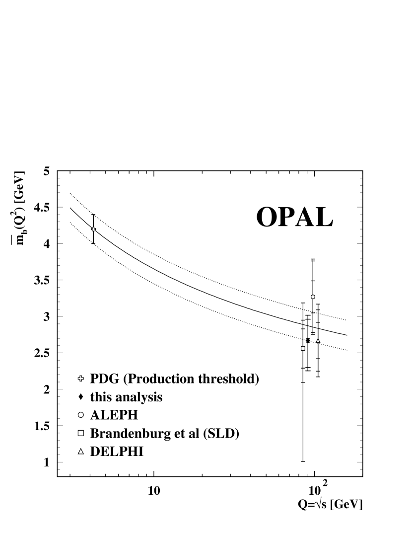
Figure 7: Results for $\overline{m}_{\mathrm{b}}(m_{\mathrm{Z}})$ from this analysis and at the scale $\overline{m}_{\mathrm{b}}$ from the compilation in [4], together with other determinations at the $\mathrm{Z}$ mass scale from DELPHI [9], ALEPH [10] and Brandenburg et al. [11]. The solid curve shows the theory expectation for the running of the b quark mass, Eq.(2), using $\alpha_{\rm S}(m_{\mathrm{Z}}^{2})=0.1184$ [32] and $\overline{m}_{\mathrm{b}}^{(\mathrm{PDG})}(\overline{m}_{\mathrm{b}})=4.2{\mathrm{~{}GeV}}$ [4]. The dotted lines display the total uncertainty on the b quark mass run from production threshold to the $\mathrm{Z}$ pole. This total uncertainty includes the uncertainty on the mass itself, $\overline{m}_{\mathrm{b}}^{(\mathrm{PDG})}(\overline{m}_{\mathrm{b}})=(4.2\pm 0.2){\mathrm{~{}GeV}}$ and the uncertainty on $\alpha_{\rm S}(m_{\mathrm{Z}}^{2})=0.1184\pm 0.0031$. The error bars of the data points show the statistical, the systematic and the theoretical uncertainties added in quadrature. For displaying purposes the four measurements at the Z pole have been separated.

The solid curve in Figure 7 shows the QCD expectation of a scale dependent $\mathrm{b}$ quark mass in the $\overline{\mathrm{MS}}$ renormalisation scheme, using the world average value of $\alpha_{\rm S}(m_{\mathrm{Z}}^{2})=0.1184\pm 0.0031$ [32]. Evolving our result of $\overline{m}_{\mathrm{b}}(m_{\mathrm{Z}})$ down to the b quark mass scale itself gives

$$\overline{m}_{\mathrm{b}}(\overline{m}_{\mathrm{b}})=(3.95\pm 0.04{\mathrm{~{}(stat.)}}^{+0.43}_{-0.55}{\mathrm{~{}(syst.)}}\pm 0.28{\mathrm{~{}(theo.)}}){\mathrm{~{}GeV}}\;,$$

which is in agreement with $(4.2\pm 0.2){\mathrm{~{}GeV}}$ [4].

We have also compared our result for the b quark mass at the $\mathrm{Z}$ mass scale with the combined value at production threshold, yielding

$$\overline{m}_{\mathrm{b}}^{(\mathrm{PDG})}(\overline{m}_{\mathrm{b}})-\overline{m}_{\mathrm{b}}(m_{\mathrm{Z}})=(1.53\pm 0.39){\mathrm{~{}GeV}}\;,$$ (15)

which is different from zero by 3.9 standard deviations, confirming the running of the b quark mass in the $\overline{\mathrm{MS}}$  renormalisation scheme as predicted by QCD.

Acknowledgements:

We thank A.Brandenburg for valuable discussion. We particularly wish to thank the SL Division for the efficient operation of the LEP accelerator at all energies and for their continuing close cooperation with our experimental group. We thank our colleagues from CEA, DAPNIA/SPP, CE-Saclay for their efforts over the years on the time-of-flight and trigger systems which we continue to use. In addition to the support staff at our own institutions we are pleased to acknowledge the
Department of Energy, USA,
National Science Foundation, USA,
Particle Physics and Astronomy Research Council, UK,
Natural Sciences and Engineering Research Council, Canada,
Israel Science Foundation, administered by the Israel Academy of Science and Humanities,
Minerva Gesellschaft,
Benoziyo Center for High Energy Physics,
Japanese Ministry of Education, Science and Culture (the Monbusho) and a grant under the Monbusho International Science Research Program,
Japanese Society for the Promotion of Science (JSPS),
German Israeli Bi-national Science Foundation (GIF),
Bundesministerium für Bildung und Forschung, Germany,
National Research Council of Canada,
Research Corporation, USA,
Hungarian Foundation for Scientific Research, OTKA T-029328, T023793 and OTKA F-023259.

References

- [1]
- [2] R.K. Ellis, W.J. Stirling and B.R. Webber: QCD and Collider Physics, Cambridge University Press, ISBN 0 521 58189 3.
- [3] J.A.M. Vermaseren, S.A. Larin and T. van Ritbergen: Phys. Lett. B405 (1997) 327.
- [4] D.E. Groom et al.: Eur. Phys. J. C15 (2000) 1.
-
[5]
ALEPH Coll., D. Buskulic et al.: Phys. Lett. B355 (1995) 381;
DELPHI Coll., P. Abreu et al.: Phys. Lett. B307 (1993) 221;
DELPHI Coll., P. Abreu et al.: Phys. Lett. B418 (1998) 430;
L3 Coll., B. Adeva et al.: Phys. Lett. B271 (1991) 461;
OPAL Coll., R. Akers et al.: Z. Phys. C60 (1993) 397;
OPAL Coll., R. Akers et al.: Z. Phys. C65 (1995) 31;
OPAL Coll., G. Abbiendi et al.: Eur. Phys. J. C11 (1999) 643;
SLD Coll., K. Abe et al.: Phys. Rev. D53 (1996) 2271;
SLD Coll., K. Abe et al.: Phys. Rev. D59 (1999) 012002. -
[6]
W. Bernreuther, A. Brandenburg and P. Uwer:
Phys. Rev. Lett. 79 (1997) 189;
A. Brandenburg and P. Uwer: Nucl. Phys. B515 (1998) 279. -
[7]
G. Rodrigo, A. Santamaria and M. Bilenky:
Phys. Rev. Lett. 79 (1997) 193;
G. Rodrigo, M. Bilenky and A. Santamaria: Nucl. Phys. B554 (1999) 257. - [8] P. Nason and C. Oleari: Nucl. Phys. B521 (1998) 237.
- [9] DELPHI Coll., P. Abreu et al.: Phys. Lett. B418 (1998) 430.
- [10] ALEPH Coll., R. Barate et al.: Eur. Phys. J. C18 (2000) 1.
- [11] A. Brandenburg, P.N. Burrows, D. Muller, N. Oishi and P. Uwer: Phys. Lett. B468 (1999) 168.
-
[12]
OPAL Coll., K. Ahmet et al.: Nucl. Inst. and Meth. A305 (1991) 275;
O. Biebel et al.: Nucl. Inst. and Meth. A323 (1992) 169. - [13] OPAL Coll., M.Z. Akrawy et al.: Phys. Lett. B253 (1991) 511.
- [14] OPAL Coll., G. Alexander et al.: Z. Phys. C52 (1991) 175.
-
[15]
P. Allport et al.: Nucl. Inst. and Meth. A346 (1994) 476;
S. Anderson et al.: Nucl. Inst. and Meth. A403 (1998) 326. - [16] OPAL Coll., G. Alexander et al.: Z. Phys. C72 (1996) 191.
- [17] OPAL Coll., K. Ackerstaff et al.: Eur. Phys. J. C2 (1998) 213.
- [18] T. Sjöstrand: Comp. Phys. Comm. 82 (1994) 74.
-
[19]
OPAL Coll., M.Z. Akrawy et al.: Z. Phys. C47 (1990) 505;
OPAL Coll., G. Alexander et al.: Z. Phys. C69 (1995) 543. - [20] J. Allison et al.: Nucl. Inst. and Meth. A317 (1992) 47.
- [21] C. Peterson, D. Schlatter, I. Schmitt and P. Zerwas: Phys. Rev. D27 (1983) 105.
- [22] OPAL Coll., G. Abbiendi et al.: Phys. Lett. B492 (2000) 13.
- [23] ALEPH, DELPHI, L3, OPAL, CDF and SLD Collaborations: “Combined results on b-hadron production rates, lifetimes, oscillations and semileptonic decays” CERN-EP-2000-096.
- [24] OPAL Coll., G. Abbiendi et al.: Eur. Phys. J. C8 (1999) 217.
- [25] OPAL Coll., R. Akers et al.: Z. Phys. C65 (1995) 17.
- [26] OPAL Coll., R. Akers et al.: Z. Phys. C63 (1994) 181.
- [27] JADE Coll., W. Bartel et al.: Z. Phys. C33 (1986) 23.
- [28] S. Bethke, Z. Kunszt, D.E. Soper and W.J. Stirling: Nucl. Phys. B370 (1992) 310, erratum ibid. B523 (1998) 681.
- [29] Yu. L. Dokshitzer, G. D. Leder, S. Moretti and B. R. Webber: JHEP 9708 (1997) 1.
- [30] M. Bilenky, S. Cabrera, J. Fuster, S. Marti, G. Rodrigo and A. Santamaria: Phys. Rev. D60 (1999) 114006.
- [31] A. Brandenburg, private communication
- [32] S. Bethke: J. Phys. G26 (2000) R27.
- [33] V. G. Kartvelishvili, A. K. Likhoded and V. A. Petrov: Phys. Lett. B78 (1978) 615.
- [34] P. D. B. Collins and T. P. Spiller: J. Phys. G11 (1985) 1289.
- [35] B.L. Ioffe: Phys. Lett. B78 (1978) 277.
- [36] G. Marchesini et al.: Comput. Phys. Commun. 67 (1992) 465.
- [37] OPAL Coll., P. Acton et al.: Z. Phys. C59 (1993) 1.