Measurement of the $CP$ Violation Parameter $\sin{}2\phi_{1}$ in $B^{0}_{d}$ Meson Decays

Abstract

We present a measurement of the Standard Model $CP$ violation parameter $\sin 2\phi_{1}$ (also known as $\sin 2\beta$) based on a $10.5~{}{\rm fb}^{-1}$ data sample collected at the $\Upsilon(4S)$ resonance with the Belle detector at the KEKB asymmetric $e^{+}e^{-}$ collider. One neutral $B$ meson is reconstructed in the $J/\psi K_{S}$, $\psi(2S)K_{S}$, $\chi_{c1}K_{S}$, $\eta_{c}K_{S}$, $J/\psi K_{L}$ or $J/\psi\pi^{0}$ $CP$-eigenstate decay channel and the flavor of the accompanying $B$ meson is identified from its charged particle decay products. From the asymmetry in the distribution of the time interval between the two $B$-meson decay points, we determine $\sin 2\phi_{1}=0.58^{+0.32}_{-0.34}({\rm stat})^{+0.09}_{-0.10}({\rm syst}).$
(submitted to Phys. Rev. Lett.)

In the Standard Model (SM), $CP$ violation arises from a complex phase in the Cabibbo-Kobayashi-Maskawa (CKM) quark mixing matrix [1]. In particular, the SM predicts a $CP$ violating asymmetry in the time-dependent rates for $B^{0}_{d}$ and $\overline{B_{d}}^{0}$ decays to a common $CP$ eigenstate, $f_{CP}$, without theoretical ambiguity due to strong interactions [2]:

$$\begin{array}[]{l}A(t)\equiv\frac{\Gamma(\overline{B_{d}}^{0}\to f_{CP})-\Gamma({B^{0}_{d}}\to f_{CP})}{\Gamma(\overline{B_{d}}^{0}\to f_{CP})+\Gamma({B^{0}_{d}}\to f_{CP})}=-\xi_{f}\sin 2\phi_{1}\sin\Delta m_{d}t,\end{array}$$

where $\Gamma(\overline{B_{d}}^{0}$ $(B_{d}^{0})$ $\to f_{CP})$ is the decay rate for a $\overline{B_{d}}^{0}(B_{d}^{0})$ to $f_{CP}$ at a proper time $t$ after production, $\xi_{f}$ is the $CP$-eigenvalue of $f_{CP}$, $\Delta m_{d}$ is the mass difference between the two $B^{0}_{d}$ mass eigenstates, and $\phi_{1}$ is one of the three internal angles of the CKM Unitarity Triangle, defined as $\phi_{1}\equiv\pi-\arg\left(\frac{-V^{*}_{tb}V_{td}}{-V^{*}_{cb}V_{cd}}\right)$ [3].

In this Letter, we report a measurement of $\sin 2\phi_{1}$ using $B^{0}_{d}\overline{B_{d}}^{0}$ meson pairs produced at the $\Upsilon(4S)$ resonance, where the two mesons remain in a coherent $p$-wave state until one of them decays. The decay of one of the $B$ mesons to a self-tagging state, $f_{tag}$, i.e. a final state that distinguishes between $B^{0}_{d}$ and $\overline{B_{d}}^{0}$, at time $t_{tag}$ projects the accompanying meson onto the opposite $b$-flavor at that time; this meson decays to $f_{CP}$ at time $t_{CP}$. The $CP$ violation manifests itself as an asymmetry $A(\Delta t)$, where $\Delta t$ is the proper time interval $\Delta t\equiv t_{CP}-t_{tag}$.

The data sample corresponds to an integrated luminosity of $10.5~{}{\rm fb}^{-1}$ collected with the Belle detector [4] at the KEKB asymmetric $e^{+}e^{-}$ (3.5 on 8 GeV) collider [5]. At KEKB, the $\Upsilon(4S)$ is produced with a Lorentz boost of $\beta\gamma=0.425$ along the electron beam direction ($z$ direction). Because the $B^{0}_{d}$ and $\overline{B_{d}}^{0}$ mesons are nearly at rest in the $\Upsilon(4S)$ center of mass system (cms), $\Delta t$ can be determined from the $z$ distance between the $f_{CP}$ and $f_{tag}$ decay vertices, $\Delta z\equiv z_{CP}-z_{tag}$, as $\Delta t\simeq\Delta z/\beta\gamma c$.

The Belle detector consists of a three-layer silicon vertex detector (SVD), a 50-layer central drift chamber (CDC), an array of 1188 aerogel ${\rm\check{C}}$erenkov counters (ACC), 128 time-of-flight (TOF) scintillation counters, and an electromagnetic calorimeter containing 8736 CsI(Tl) crystals (ECL) all located inside a 3.4-m-diameter superconducting solenoid that generates a 1.5 T magnetic field. The transverse momentum resolution for charged tracks is $(\sigma_{p_{t}}/p_{t})^{2}=(0.0019p_{t})^{2}+(0.0034)^{2}$, where $p_{t}$ is in ${\rm GeV}/c$, and the impact parameter resolutions for $p=1~{}{\rm GeV}/c$ tracks at normal incidence are $\sigma_{r\phi}\simeq\sigma_{z}=55\mu{\rm m}$. Specific ionization ($dE/dx$) measurements in the CDC ($\sigma_{dE/dx}=6.9\%$ for minimum ionizing pions), TOF flight-time measurements ($\sigma_{TOF}=95~{}{\rm ps}$), and the response of the ACC provide $K^{\pm}$ identification with an efficiency of $\sim 85\%$ and a charged pion fake rate of $\sim 10\%$ for all momenta up to $3.5~{}{\rm GeV}/c$. Photons are identified as ECL showers that have a minimum energy of 20 MeV and are not matched to a charged track. The photon energy resolution is $(\sigma_{E}/E)^{2}=(0.013)^{2}+(0.0007/E)^{2}+(0.008/E^{1/4})^{2}$, where $E$ is in GeV. Electron identification is based on a combination of CDC $dE/dx$ information, the ACC response, and the position relative to the extrapolated track, shape and energy deposit of the associated ECL shower. The efficiency is greater than $90\%$ and the hadron fake rate is $\sim 0.3\%$ for $p>1~{}{\rm GeV}/c$. An iron flux-return yoke outside the solenoid, comprised of 14 layers of 4.7-cm-thick iron plates interleaved with a system of resistive plate counters (KLM), provides muon identification with an efficiency greater than $90\%$ and a hadron fake rate less than $2\%$ for $p>1~{}{\rm GeV}/c$. The KLM is used in conjunction with the ECL to detect $K_{L}$ mesons; the angular resolution of the $K_{L}$ direction measurement ranges between $1.5^{\circ}$ and $3^{\circ}$.

We reconstruct $B^{0}_{d}$ decays to the following ${CP}$ eigenstates: $J/\psi K_{S}$, $\psi(2S)K_{S}$, $\chi_{c1}K_{S}$, $\eta_{c}K_{S}$ for $\xi_{f}=-1$ and $J/\psi\pi^{0}$, $J/\psi K_{L}$ for $\xi_{f}=+1$. The $J/\psi$ and $\psi(2S)$ mesons are reconstructed via their decays to $\ell^{+}\ell^{-}$ $(\ell=\mu,e)$. The $\psi(2S)$ is also reconstructed via its $J/\psi\pi^{+}\pi^{-}$ decay, the $\chi_{c1}$ via its $J/\psi\gamma$ decay, and the $\eta_{c}$ via its $K^{+}K^{-}\pi^{0}$ and $K_{S}(\pi^{+}\pi^{-})K^{-}\pi^{+}$ [6] decays.

For $J/\psi$ and $\psi(2S)\to\ell^{+}\ell^{-}$ decays, we use oppositely charged track pairs where both tracks are positively identified as leptons. For the $B^{0}_{d}\to J/\psi K_{S}(\pi^{+}\pi^{-})$ mode, the requirement for one of the tracks is relaxed: a track with an ECL energy deposit consistent with a minimum ionizing particle is accepted as a muon and a track that satisfies either the $dE/dx$ or the ECL shower energy requirements as an electron. For $e^{+}e^{-}$ pairs, we include the four-momentum of every photon detected within 0.05 radians of the original $e^{+}$ or $e^{-}$ direction in the invariant mass calculation. Nevertheless a radiative tail remains and we accept pairs in the asymmetric invariant mass interval between $-12.5\sigma$ and $+3\sigma$ of $M_{J/\psi}$ or $M_{\psi(2S)}$, where $\sigma=12~{}{\rm MeV}/c^{2}$ is the mass resolution. The $\mu^{+}\mu^{-}$ radiative tail is smaller; we select pairs within $-5\sigma$ and $+3\sigma$ of $M_{J/\psi}$ or $M_{\psi(2S)}$. Candidate $K_{S}\to\pi^{+}\pi^{-}$ decays are oppositely charged track pairs that have an invariant mass within $\pm 4\sigma$ of the $K^{0}$ mass ($\sigma\simeq 4~{}{\rm MeV}/c^{2}$). For the $J/\psi K_{S}$ final state, $K_{S}\to\pi^{0}\pi^{0}$ decays are also used. For $\pi^{0}\pi^{0}$ candidates, we try all combinations where there are two $\gamma\gamma$ pairs with an invariant mass between 80 and 150 ${\rm MeV}/c^{2}$, assuming they originate from the center of the run-dependent average interaction point (IP). We minimize the sum of the $\chi^{2}$ values from constrained fits of each pair to the $\pi^{0}$ mass with $\gamma$ directions determined by varying the decay point along the $K_{S}$ flight path, which is taken as the line from the IP to the energy-weighted center of the four showers. We select combinations with a $\pi^{0}\pi^{0}$ invariant mass within $\sim\pm 3\sigma$ of $M_{K^{0}}$, where $\sigma\simeq 9.3~{}{\rm MeV}/c^{2}$. For the $J/\psi\pi^{0}$ mode, we use a minimum $\gamma$ energy of 100 MeV and select $\gamma\gamma$ pairs with an invariant mass within $\pm 3\sigma$ of $M_{\pi^{0}}$, where $\sigma\simeq 4.9~{}{\rm MeV}/c^{2}$.

We isolate reconstructed $B$ meson decays using the energy difference $\Delta E\equiv E_{B}^{cms}-E_{beam}^{cms}$ and the beam-energy constrained mass $M_{bc}\equiv\sqrt{(E_{beam}^{cms})^{2}-(p_{B}^{cms})^{2}}$, where $E_{beam}^{cms}$ is the cms beam energy, and $E_{B}^{cms}$ and $p_{B}^{cms}$ are the cms energy and momentum of the $B$ candidate. Figure 1 shows the $M_{bc}$ distribution for all channels combined (other than $J/\psi K_{L}$) after a $\Delta E$ selection that varies from $\pm 25$ MeV to $\pm 100$ MeV (corresponding to $\sim\pm 3\sigma$), depending on the mode. The $B$ meson signal region is defined as $5.270<M_{bc}<5.290~{}{\rm GeV}/c^{2}$; the $M_{bc}$ resolution is $3.0~{}{\rm MeV}/c^{2}$. Table I lists the numbers of observed events ($N_{ev}$) and the background ($N_{bkgd}$) determined by extrapolating the event rate in the non-signal $\Delta E$ vs. $M_{bc}$ region into the signal region.

Candidate $B^{0}_{d}\to J/\psi K_{L}$ decays are selected by requiring the observed $K_{L}$ direction to be within $45^{\circ}$ from the direction expected for a two-body decay (ignoring the $B_{d}^{0}$ cms motion). We reduce the background by means of a likelihood quantity that depends on the $J/\psi$ cms momentum, the angle between the $K_{L}$ and its nearest-neighbor charged track, the charged track multiplicity, and the kinematics that obtain when the event is reconstructed assuming a $B^{+}\to$ $J/\psi K^{*+}(K_{L}\pi^{+})$ hypothesis. In addition, we remove events that are reconstructed as $B_{d}^{0}\to J/\psi K_{S}$, $J/\psi K^{*0}(K^{+}\pi^{-},K_{S}\pi^{0})$, $B^{+}\to$ $J/\psi K^{+}$, or $J/\psi K^{*+}(K^{+}\pi^{0}$ $K_{S}\pi^{+})$ decays. Figure 2 shows the $p_{B}^{cms}$ distribution, calculated for a $B^{0}_{d}\to J/\psi K_{L}$ two-body decay hypothesis, for the surviving events. The histograms in the figure are the results of a fit to the signal and background distributions, where the shapes are derived from Monte Carlo simulations (MC) [7], and the normalizations are allowed to vary. Among the total of 131 entries in the $0.2\leq p_{B}^{cms}\leq 0.45~{}{\rm GeV}/c$ signal region, the fit finds 77 $J/\psi K_{L}$ events.

The leptons and charged pions and kaons among the tracks that are not associated with $f_{CP}$ are used to identify the flavor of the accompanying $B$ meson. Tracks are selected in several categories that distinguish the $b$-flavor by the track’s charge: high momentum leptons from $b\to c\ell^{-}\overline{\nu}$, lower momentum leptons from $c\to s\ell^{+}\nu$, charged kaons from $b\to c\to s$, high momentum pions from decays of the type $B_{d}^{0}\to D^{(*)-}(\pi^{+},\rho^{+},a_{1}^{+},{\rm etc.})$, and slow pions from $D^{*-}\to\overline{D}^{0}\pi^{-}$. For each track in one of these categories, we use the MC to determine the relative probability that it originates from a $B^{0}_{d}$ or $\overline{B_{d}}^{0}$ as a function of its charge, cms momentum and polar angle, particle-identification probability, and other kinematic and event shape quantities. We combine the results from the different track categories (taking into account correlations for the case of multiple inputs) to determine a $b$-flavor $q$, where $q=+1$ when $f_{tag}$ is more likely to be a $B^{0}_{d}$ and $-1$ for a $\overline{B_{d}}^{0}$. We use the MC to evaluate an event-by-event flavor-tagging dilution factor, $r$, which ranges from $r=0$ for no flavor discrimination to $r=1$ for perfect flavor assignment. We only use $r$ to categorize the event. For the $CP$ asymmetry analysis, we use the data to correct for wrong-flavor assignments.

The probabilities for an incorrect flavor assignment, $w_{l}\ (l=1,6)$, are measured directly from the data for six $r$ intervals using a sample of exclusively reconstructed, self-tagged $B^{0}_{d}\to D^{*-}\ell^{+}\nu$, $D^{(*)-}\pi^{+}$, and $D^{*-}\rho^{+}$ decays. The $b$-flavor of the accompanying $B$ meson is assigned according to the above-described flavor-tagging algorithm, and values of $w_{l}$ are determined from the amplitudes of the time-dependent $B^{0}_{d}$-$\overline{B_{d}}^{0}$ mixing oscillations [8]: $(N_{OF}-N_{SF})/(N_{OF}+N_{SF})=(1-2w_{l})\cos(\Delta m_{d}\Delta t)$. Here $N_{OF}$ and $N_{SF}$ are the numbers of opposite and same flavor events. Table II lists the resulting $w_{l}$ values together with the fraction of the events ($f_{l}$) in each $r$ interval. All events in Table I fall in one of the six $r$ intervals. The total effective tagging efficiency is $\sum_{l}f_{l}(1-2w_{l})^{2}=0.270^{+0.021}_{-0.022}$, where the error includes both statistical and systematic uncertainties, in good agreement with the MC result of 0.274. We check for a possible bias in the flavor tagging by measuring the effective tagging efficiency for $B_{d}^{0}$ and $\overline{B_{d}}^{0}$ self-tagged samples separately, and for different $\Delta t$ intervals. We find no statistically significant difference.

The vertex positions for the $f_{CP}$ and $f_{tag}$ decays are reconstructed using tracks that have at least one 3-dimensional coordinate determined from associated $r\phi$ and $z$ hits in the same SVD layer plus one or more additional $z$ hits in other SVD layers. Each vertex position is required to be consistent with the IP profile smeared in the $r\phi$ plane by the $B$ meson decay length. (The IP size, determined run-by-run, is typically $\sigma_{x}\simeq 100~{}\mu{\rm m}$, $\sigma_{y}\simeq 5~{}\mu{\rm m}$ and $\sigma_{z}\simeq 3~{}{\rm mm}$.) The $f_{CP}$ vertex is determined using lepton tracks from the $J/\psi$ or $\psi(2S)$ decays, or prompt tracks from $\eta_{c}$ decays. The $f_{tag}$ vertex is determined from tracks not assigned to $f_{CP}$ with additional requirements of $\delta r<0.5~{}{\rm mm}$, $\delta z<1.8~{}{\rm mm}$ and $\sigma_{\delta z}<0.5~{}{\rm mm}$, where $\delta r$ and $\delta z$ are the distances of the closest approach to the $f_{CP}$ vertex in the $r\phi$ plane and the $z$ direction, respectively, and $\sigma_{\delta z}$ is the calculated error of $\delta z$. Tracks that form a $K_{S}$ are removed. The MC indicates that the average $z_{CP}$ resolution is $75~{}\mu{\rm m}~{}({\rm rms})$; the $z_{tag}$ resolution is worse ($140~{}\mu{\rm m}$) because of the lower average momentum of the $f_{tag}$ decay products and the smearing caused by secondary tracks from charmed meson decays.

The resolution function $R(\Delta t)$ for the proper time interval is parameterized as a sum of two Gaussian components: a main component due to the SVD vertex resolution, charmed meson lifetimes and the effect of the cms motion of the $B$ mesons, plus a tail component caused by poorly reconstructed tracks. The means ($\mu_{main}$, $\mu_{tail}$) and widths ($\sigma_{main}$, $\sigma_{tail}$) of the Gaussians are calculated event-by-event from the $f_{CP}$ and $f_{tag}$ vertex fit error matrices; average values are $\mu_{main}=-0.09~{}{\rm ps}$, $\mu_{tail}=-0.78~{}{\rm ps}$ and $\sigma_{main}=1.54~{}{\rm ps}$, $\sigma_{tail}=3.78~{}{\rm ps}$. The negative values of the means are due to secondary tracks from charmed mesons. The relative fraction of the main Gaussian is determined to be $0.982\pm 0.013$ from a study of $B^{0}_{d}\to D^{*-}\ell^{+}\nu$ events. The reliability of the $\Delta t$ determination and $R(\Delta t)$ parameterization is confirmed by lifetime measurements of the neutral and charged $B$ mesons [9] that use the same procedures and are in good agreement with the world average values [10].

We determine $\sin 2\phi_{1}$ from an unbinned maximum-likelihood fit to the observed $\Delta t$ distributions. The probability density function (pdf) expected for the signal distribution is given by

$${\cal P}_{sig}(\Delta t,q,w_{l},\xi_{f}) = \frac{e^{-|\Delta t|/\tau_{B^{0}_{d}}}}{2\tau_{B^{0}_{d}}}\{1-\xi_{f}q(1-2w_{l})\sin 2\phi_{1}\sin(\Delta m_{d}\Delta t)\},$$

where we fix the $B^{0}_{d}$ lifetime and mass difference at their world average values [10]. The pdf used for background events is ${\cal P}_{bkg}(\Delta t)=f_{\tau}e^{-|\Delta t|/\tau_{bkg}}/2\tau_{bkg}+(1-f_{\tau})\delta(\Delta t),$ where $f_{\tau}$ is the fraction of the background component with an effective lifetime $\tau_{bkg}$ and $\delta(\Delta t)$ is the Dirac delta function. For all $f_{CP}$ modes except $J/\psi K_{L}$ we find $f_{\tau}=0.10^{+0.11}_{-0.05}$ and $\tau_{bkg}=1.75^{+1.15}_{-0.82}~{}{\rm ps}$ using events in background-dominated regions of $\Delta E$ vs. $M_{bc}$. The $J/\psi K_{L}$ background is dominated by $B\to J/\psi X$ decays, where some final states are $CP$ eigenstates and need special treatment. A MC study shows that the background contribution from the $\xi_{f}=-1$ sources $J/\psi K_{S}$, $\psi(2S)K_{S}$ and $\chi_{c1}K_{S}$ is 7.9%, while that from the $\xi_{f}=+1$ $\psi(2S)K_{L}$ and $\chi_{c1}K_{L}$ modes is $7.0\%$. Thus, the effects on the $CP$ asymmetry from these states nearly cancel. The remaining dominant $CP$ mode, $J/\psi K^{*}(K_{L}\pi^{0})$, which accounts for 19% of the total background, is taken to be a $73/27$ mixture of $\xi_{f}=-1$ and $+1$, respectively, based on our measurement of the $J/\psi$ polarization in the $B_{d}^{0}\to J/\psi K^{*0}(K_{S}\pi^{0})$ decay [11]. For the $J/\psi K^{*}(K_{L}\pi^{0})$ background pdf we use ${\cal P}_{sig}$ with effective $CP$ eigenvalue $\xi_{f}=-0.46^{+1.46}_{-0.54}$, where the error has been expanded to include all possible values. For the non-$CP$ background modes we use ${\cal P}_{bkg}$ with $f_{\tau}=1$ and $\tau_{bkg}=\tau_{B}$.

The pdfs are convolved with $R(\Delta t)$ to determine the likelihood value for each event as a function of $\sin 2\phi_{1}$:

$${\cal L}_{i} = {\displaystyle\int}\{f_{sig}{\cal P}_{sig}(\Delta t^{\prime},q,w_{l},\xi_{f})+(1-f_{sig}){\cal P}_{bkg}(\Delta t^{\prime})\}R(\Delta t-\Delta t^{\prime})d\Delta t^{\prime},$$

where $f_{sig}$ is the probability that the event is signal, calculated as a function of $p_{B}^{cms}$ for $J/\psi K_{L}$ and of $\Delta E$ and $M_{bc}$ for other modes. The most probable $\sin 2\phi_{1}$ is the value that maximizes the likelihood function $L=\prod_{i}{\cal L}_{i}$, where the product is over all events. We performed a blind analysis: the fitting algorithms were developed and finalized using a flavor-tagging routine that does not divulge the sign of $q$. The sign of $q$ was then turned on and the application of the fit to all the events listed in Table I produces the result $\sin 2\phi_{1}=0.58^{+0.32+0.09}_{-0.34-0.10}$, where the first error is statistical and the second systematic. The systematic errors are dominated by the uncertainties in $w_{l}$ (${}^{+0.05}_{-0.07}$) and the $J/\psi K_{L}$ background ($\pm 0.05$). Separate fits to the $\xi_{f}=-1$ and $\xi_{f}=+1$ event samples give $0.82^{+0.36}_{-0.41}$ and $0.10^{+0.57}_{-0.60}$, respectively [12]. Figure 3(a) shows $-2\ln(L/L_{max})$ as a function of $\sin 2\phi_{1}$ for the $\xi_{f}=-1$ and $\xi_{f}=+1$ modes separately and for both modes combined. Figure 3(b) shows the asymmetry obtained by performing the fit to events in $\Delta t$ bins separately, together with a curve that represents $\sin 2\phi_{1}\sin(\Delta m_{d}\Delta t)$ for $\sin 2\phi_{1}=0.58$.

We check for a possible fit bias by applying the same fit to non-$CP$ eigenstate modes: $B^{0}_{d}\rightarrow D^{(*)-}\pi^{+}$, $D^{*-}\rho^{+}$, $J/\psi K^{*0}(K^{+}\pi^{-})$, and $D^{*-}\ell^{+}\nu$, where “$\sin 2\phi_{1}$” should be zero, and the charged mode $B^{+}\to J/\psi K^{+}$. For all the modes combined we find $0.065\pm 0.075$, consistent with a null asymmetry.

We have presented a measurement of the Standard Model $CP$ violation parameter $\sin 2\phi_{1}$ based on a $10.5~{}{\rm fb}^{-1}$ data sample collected at the $\Upsilon(4S)$:

$$\sin 2\phi_{1}=0.58^{+0.32}_{-0.34}({\rm stat})^{+0.09}_{-0.10}({\rm syst}).$$

The probability of observing $\sin 2\phi_{1}>0.58$ if the true value is zero is $4.9\%$. Our measurement is more precise than the previous measurements [13] and consistent with SM constraints [14].

We wish to thank the KEKB accelerator group for the excellent operation. We acknowledge support from the Ministry of Education, Culture, Sports, Science and Technology of Japan and the Japan Society for the Promotion of Science; the Australian Research Council and the Australian Department of Industry, Science and Resources; the Department of Science and Technology of India; the BK21 program of the Ministry of Education of Korea and the SRC program of the Korea Science and Engineering Foundation; the Polish State Committee for Scientific Research under contract No.2P03B 17017; the Ministry of Science and Technology of Russian Federation; the National Science Council and the Ministry of Education of Taiwan; the Japan-Taiwan Cooperative Program of the Interchange Association; and the U.S. Department of Energy.

TABLE I.: The numbers of $CP$ eigenstate events

Mode	$N_{ev}$	$N_{bkgd}$
$J/\psi(\ell^{+}\ell^{-})K_{S}(\pi^{+}\pi^{-})$	123	3.7
$J/\psi(\ell^{+}\ell^{-})K_{S}(\pi^{0}\pi^{0})$	19	2.5
$\psi(2S)(\ell^{+}\ell^{-})K_{S}(\pi^{+}\pi^{-})$	13	0.3
$\psi(2S)(J/\psi\pi^{+}\pi^{-})K_{S}(\pi^{+}\pi^{-})$	11	0.3
$\chi_{c1}(\gamma J/\psi)K_{S}(\pi^{+}\pi^{-})$	3	0.5
$\eta_{c}(K^{+}K^{-}\pi^{0})K_{S}(\pi^{+}\pi^{-})$	10	2.4
$\eta_{c}(K_{S}K^{+}\pi^{-})K_{S}(\pi^{+}\pi^{-})$	5	0.4
$J/\psi(\ell^{+}\ell^{-})\pi^{0}$	10	0.9
Sub-total	194	11
$J/\psi(\ell^{+}\ell^{-})K_{L}$	131	54

TABLE II.: Experimentally determined event fractions ($f_{l}$) and incorrect flavor assignment probabilities ($w_{l}$) for each $r$ interval.

$l$	$r$	$f_{l}$	$w_{l}$
1	$0.000-0.250$	$0.393\pm 0.014$	$0.470^{+0.031}_{-0.035}$
2	$0.250-0.500$	$0.154\pm 0.007$	$0.336^{+0.039}_{-0.042}$
3	$0.500-0.625$	$0.092\pm 0.005$	$0.286^{+0.037}_{-0.035}$
4	$0.625-0.750$	$0.100\pm 0.005$	$0.210^{+0.033}_{-0.031}$
5	$0.750-0.875$	$0.121\pm 0.006$	$0.098^{+0.028}_{-0.026}$
6	$0.875-1.000$	$0.134\pm 0.006$	$0.020^{+0.023}_{-0.019}$

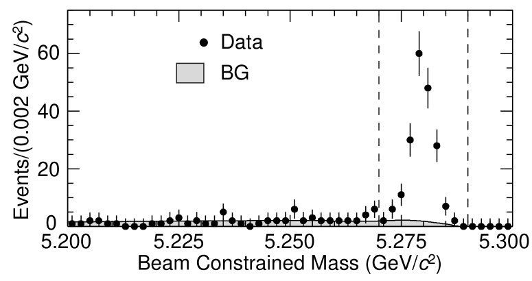
FIG. 1.: The beam-constrained mass distribution for all decay modes combined (other than $B^{0}_{d}\to J/\psi K_{L}$). The shaded area is the estimated background. The dashed lines indicate the signal region.

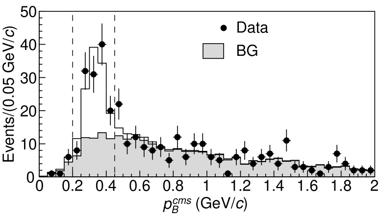
FIG. 2.: The $p_{B}^{cms}$ distribution for $B^{0}_{d}\to J/\psi K_{L}$ candidates with the results of the fit. The solid line is the signal plus background; the shaded area is background only. The dashed lines indicate the signal region.

FIG. 3.: (a) Values of $-2\ln(L/L_{max})$ vs. $\sin 2\phi_{1}$ for the $\xi_{f}=-1$ and $+1$ modes separately and for both modes combined. (b) The asymmetry obtained from separate fits to each $\Delta t$ bin; the curve is the result of the global fit ($\sin 2\phi_{1}=0.58$).

REFERENCES

[1]
M. Kobayashi and T. Maskawa, Prog. Theor. Phys. 49, 652 (1973).
[2]
A.B. Carter and A.I. Sanda, Phys. Rev. D23, 1567 (1981);
I.I. Bigi and A.I. Sanda, Nucl. Phys. B193, 85 (1981).
[3]
H. Quinn and A.I. Sanda, Eur. Phys. Jour. C15, 626 (2000).
(Some papers refer to this angle as .)
[4]
K. Abe et al. (Belle Collab.),
The Belle Detector, KEK Report 2000-4, to be published
in Nucl. Instrum. Methods.
[6]
Throughout this Letter, when a mode is quoted the inclusion of the charge
conjugate mode is implied.
[7]
We use the QQ meson decay event generator
developed by the CLEO collaboration (http://www.lns.cornell.edu/public/CLEO/soft/QQ)
and GEANT3 for the detector simulation;
CERN Program Library Long Writeup W5013, CERN, 1993.
[8]
J. Suzuki (Belle Collab.), Determination of - Mixing from The Time
Evolution of Dilepton and Events at Belle,
Proceedings of the 30th International Conference on High Energy
Physics, July 2000, Osaka.
[9]
H. Tajima (Belle Collab.), Measurement of Heavy Meson
Lifetimes with Belle, ibid.
[11]
Belle Collab., Measurement of Polarization of in
and
Decays, Contributed paper (#285) to
the 30th International Conference on High Energy Physics,
July 2000, Osaka.
This result agrees within errors with those of
C.P Jessop et al. (CLEO Collab.), Phys. Rev. Lett. 79, 4533 (1997) and
T. Affolder et al. (CDF Collab.), Phys. Rev. Lett. 85, 4668 (2000).
[12]
A fit to only the events
gives a value of ;
a fit to only the non- modes gives .
Separate fits to the and event samples
give values of and ,
respectively.
[13]
K. Ackerstaff et al. (OPAL Collab.), Eur. Phys. Jour. C5, 379 (1998);
T. Affolder et al. (CDF Collab.), Phys. Rev. D61
072005 (2000); and
R. Barate et al. (ALEPH Collab.), Phys. Lett. B492, 259 (2000).
[14]
For example: S. Mele, Phys. Rev. D59, 113011 (1999).