EXPERIMENTAL CORRELATION ANALYSIS:
FOUNDATIONS AND PRACTICE

Abstract

Commonalities and differences in correlation analysis in terms of phase space, conditioning and uncorrelatedness are discussed. The Poisson process is not generally appropriate as reference distribution for normalisation and cumulants, so that generalised statistics in terms of arbitrarily defined reference processes must be employed. Consideration of the sampling hierarchy leads us to a classification of current event-by-event observables.

1 Introduction

In theory, knowledge of the fully differential probability distribution at all points contains everything there is to know about a given reaction. While this statement may be true, it is meaningless in practice because experimental samples are invariably too small to access even a fraction of the required information; also, the dimension of phase space is large, creating problems of projection and visualisation.

In this situation, multiparticle correlations provide meaningful answers through inclusive sampling: projectiles $A$ and $B$ collide to yield $N$ final-state particles, of which the observer considers only $q$ particles at a time, $A+B\longrightarrow p_{1}+p_{2}+\cdots+p_{q}+X$, while ignoring the rest $X$ by means of final-state phase space integration. In the simplest case $q{=}0$, one considers the multiplicity and the size of the available phase space,[1] advancing to one-particle distributions ($q{=}1$), two-particle correlations ($q{=}2$) and so forth. Every step on the $q$-ladder presents new and increasingly subtle challenges, both physicswise and in statistical sophistication. This review hopes to highlight both the simplicity and unity that a rigorous mathematical approach has taught us.

2 Phase space and conditioning

Data to be analysed typically consists of a sample $S$ of events $e=1,2,\ldots,{\cal N}_{\rm ev}$, each with a different multiplicity $\hat{N}^{e}$ of tracks, each of which has momentum and other measured quantum numbers contained in a vector $X_{i}^{e},i=1,\ldots\hat{N}^{e}$. For $q$-th order correlation measurement, the sample is completely described by the set of per-event counter densities, one for each event,

$$\hat{\rho}_{q}(x_{1},\ldots,x_{q})=\sum_{\stackrel{{\scriptstyle\scriptstyle i_{1}\neq i_{2}\neq\cdots}}{{\scriptstyle\neq i_{q}=1}}}^{\hat{N}}f(X^{e}_{i_{1}},X^{e}_{i_{2}},\ldots,X^{e}_{i_{q}})\;\delta(x_{1}-X^{e}_{i_{1}})\cdots\delta(x_{q}-X^{e}_{i_{q}})\,,$$ (1)

which registers a value $f_{1}(x_{1},\ldots,x_{q})$ whenever the coordinates $(X^{e}_{i_{1}},\ldots,X^{e}_{i_{q}})$ of an ordered data $q$-tuple exactly match the observation points $(x_{1},\ldots,x_{q})$. Some simple examples for $\hat{\rho}_{q}$ and $f$ are the all-charge rapidity counter $\hat{\rho}_{1}(y)=\sum_{i=1}^{\hat{N}}\delta(y-y_{i})$ with $f\equiv 1$, and, using a 4-dimensional $\mathbf{X}^{e}_{i}\equiv(y_{i},\phi_{i},p_{\bot\,i},c_{i})$ with charges $c_{i}=\pm 1$, a second-order positives-only counter $\hat{\rho}_{2}(\mathbf{x}_{1}^{+},\mathbf{x}_{2}^{+})=\sum_{i\neq j}\delta_{c_{i},1}\delta_{c_{j},1}\;\delta(\mathbf{x}_{1}-\mathbf{X}^{e}_{i})\;\delta(\mathbf{x}_{2}-\mathbf{X}^{e}_{j})$ or a charge-charge counter $\hat{\rho}_{2}(\mathbf{x}_{1},\mathbf{x}_{2})=\sum_{i\neq j}c_{i}c_{j}\;\delta(\mathbf{x}_{1}-\mathbf{X}^{e}_{i})\;\delta(\mathbf{x}_{2}-\mathbf{X}^{e}_{j})$.

Essentially all correlation measures can be represented as combinations of the two kinds of averages over $\hat{\rho}_{q}(x_{1},\ldots,x_{q})$ shown in Figure 1:

1. “spatial” averaging, in the form of phase space integrals $\int_{\Omega}dx_{1}\,dx_{2}\,\ldots dx_{q}$ of the arguments $x$ over a selected region of phase space $\Omega$, and

2. sample averaging $\langle\ \rangle_{S}=(1/{\cal N}_{\rm ev})\sum_{e}$ over a sample $S$.

Figure 1: Phase space and event averaging of the per-event counter $\hat{\rho}_{q}$ yields, respectively, the per-event factorial moment $\hat{N}^{[q]}=\hat{N}(\hat{N}{-}1)\cdots(\hat{N}{-}q{+}1)$, the correlation density $\rho_{q}(x_{1},\ldots,x_{q})$ and the sample factorial moment $\langle N^{[q]}\rangle$ for a particular choice of $\Omega$ and $S$.

Along with the choice of variable $x$ and weight function $f$, the choice of phase space $\Omega$ and sample $S$ over which to average is motivated by the physics under investigation. Choice of $\Omega$ concerns particle selection; choice of $S$, called conditioning, concerns event selection.

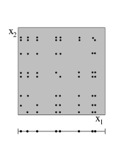
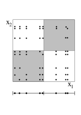
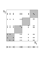
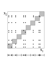
Figure 2: Phase space integration domains $\Omega$ (shaded areas) for various stages of box intermittency analysis. Each point represents a particle 2-tuple (pair) of the event whose tracks are represented as dots on the line below the phase space plot. Also shown is the corresponding increasingly fine binning of the event.

We focus first on $\Omega$. In Figure 2, we show, for the old box-moment intermittency analysis, the appropriate $\Omega$’s as shaded areas, for various resolutions $L/2^{j}$, superimposed on an example counter $\hat{\rho}_{2}(x_{1},x_{2})$, each of whose dots represents a pair drawn from the $\hat{N}=8$ tracks shown on the line below the plot itself. Further examples of $\Omega$ for $\hat{\rho}_{2}(y_{1},y_{2})$ for fixed $y_{1}$ and the differential correlation integral [2] over the same counter are shown in Figs. 3a and 3b respectively; greyscales represent the $\Omega$’s for successive data points. The correlation density $\rho_{q}(x_{1},\ldots,x_{q})=\langle\hat{\rho}_{q}\rangle$, which for $q=2$ is conveniently represented as a two-dimensional contour plot, is shown schematically in Figs. 3c and 3d for rapidity $y$, together with $\Omega$’s for forward-backward and rapidity gap measurements.

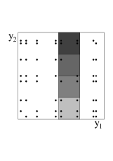
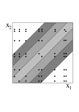
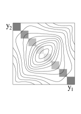
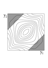
(a)

(b)

(c)

(d)

Figure 3: Examples of phase space integrals over $\Omega$. From left to right: (a) box correlations keeping rapidity $y_{1}$ fixed; (b) correlation integral with linear binning in $|x_{1}-x_{2}|$; (c) forward-backward correlations for fixed bin widths but varying bin-bin separation; (d) rapidity gap correlations.

There is freedom of choice in sample averaging also. “Conditioning” is the choosing of a subsample of events from the available full sample according to some criterion $I_{C}$ based on attribute $\hat{C}$, such as an interval $I_{C}\equiv\{C\in[C_{min},C_{max}]\}$. Examples of conditioning are overall multiplicity ($\hat{C}=\hat{N}(\Omega_{\rm tot})$), tagging ($\hat{C}$ = some quantum number), central collision selections, and kaon-to-pion ratio.

The influence of conditioning appears to be obvious and quite limited, in that different (sub)samples will clearly yield different results, and so little attention has been paid to it. This is deceptive, however: conditioning, or rather its absence, directly enters the foundations of correlation analysis as a hidden assumption and is therefore of central importance.

3 Uncorrelatedness

Experimental correlation analysis needs to be both measurable and meaningful. It is measurable only as far as trivial contributions to the correlated signal can be successfully eliminated; it is meaningful only to the extent that implicit assumptions are understood and fulfilled. Elimination of trivialities is accomplished in part by cumulants and appropriate normalisation, while consideration of an assumption underlying uncorrelatedness, the absence of correlation, will lead us to the “reference distribution”.

3.1 Cumulants

Moments $\hat{N}^{q}$ and factorial moments $\hat{N}^{[q]}$, whether per-event or sample-averaged, contain correlations of all orders $\leq q$ and so are very bad indicators of correlation of order $q$ itself. These trivial lower-order contributions are removed by the use of cumulants, which are thus generally preferable. Important for our purposes are two well-known cumulant properties:

• Behaviour under statistical independence: A differential cumulant (e.g. $C_{2}(x_{1},x_{2})=\rho_{2}(x_{1},x_{2})-\rho_{1}(x_{1})\rho_{1}(x_{2})$) becomes zero whenever any one of its $q$ arguments is statistically independent of (uncorrelated with respect to) the others, and the integrated factorial cumulant (e.g. $\langle N(N{-}1)\rangle-\langle N\rangle^{2}$) is zero when the distribution in $\Omega$ is poissonian:

  $$C_{q}(x_{1},\ldots,x_{q}) \stackrel{{\scriptstyle\mbox{{\ \scriptsize statistical independence\ }}}}{{\begin{picture}(100.0,3.0)\put(0.0,3.0){\leavevmode} \end{picture}}}\;0\,,$$ (2)

  $$\int_{\Omega}C_{q}(x_{1},\ldots,x_{q})\,dx_{1}\cdots dx_{q} \stackrel{{\scriptstyle\mbox{{\ \scriptsize Poissonian in $\Omega$\ }}}}{{\begin{picture}(80.0,3.0)\put(0.0,3.0){\leavevmode} \end{picture}}}\;0\,.$$ (3)

• Additivity: If two distributions $P_{f}$ and $P_{h}$ are independent, the cumulant of the convolved distribution is the arithmetic sum of the individual cumulants,

  $$C_{q}^{(f*h)}=C_{q}^{(f)}+C_{q}^{(h)}\,.$$ (4)

There is a problem, however: While eq. (3) is true and seems simple enough, it assumes implicitly that the sample $S$ (i) is inclusive, and (ii) has an overall poissonian multiplicity distribution $P_{\hat{N}}=e^{-\nu}\nu^{\hat{N}}/\hat{N}!$. A sample for which these assumptions are not fulfilled (i.e. almost every conditioned sample!) will hence not yield zero cumulants, even when it is otherwise considered “uncorrelated” by the naive user. Indeed, it has long been a source of consternation that for fixed-multiplicity samples, $P_{\hat{N}}=\delta_{\hat{N},N_{\rm fix}}$, the cumulant does not integrate to zero, $\int dx_{1}\,dx_{2}\,C_{2}=\int dx_{1}\,dx_{2}(\rho_{2}-\rho_{1}^{2})=N(N{-}1)-N^{2}=-N$; similarly, the nonpoissonian overall multiplicity of UA1 data is known to be the source of nonzero $C_{2}(\Omega_{\rm tot})_{\rm UA1}\simeq 0.4$.

For the stronger condition (2) to be fulfilled, the uncorrelated sample needs to be a realisation of the Poisson process, for which both $P_{\hat{N}}$ is poissonian and all possible subdivisions of phase space are both mutually uncorrelated and poissonian in themselves.

3.2 Normalisation

Normalisation is designed to get rid of the trivial dependence on the overall multiplicity (leaving nontrivial multiplicity-driven effects) and the shape of the one-particle distribution. Both trivial multiplicity dependence and shape are eliminated by the “vertical” or differential normalisation $\rho_{1}(x_{1})\cdots\rho_{1}(x_{q})$, which is commonly held to be appropriate because for uncorrelated samples $\rho_{q}\to\rho_{1}\cdots\rho_{1}$ and so

$$r_{q}(x_{1},\ldots,x_{q})={\rho_{q}(x_{1},\ldots,x_{q})\over\rho_{1}(x_{1})\cdots\rho_{1}(x_{q})}\stackrel{{\scriptstyle\mbox{{\ \scriptsize statistical independence\ }}}}{{\begin{picture}(100.0,3.0)\put(0.0,3.0){\leavevmode} \end{picture}}}\;1\,.$$ (5)

Again, however, this normalisation turns out to be incorrect for any conditioned sample; again, the implicit assumption being made in writing $\rho_{q}\to\rho_{1}^{q}$ is that the uncorrelated case is the Poisson process, which is clearly impossible once conditioning changes $P_{\hat{N}}$. Most experimentalists are intuitively aware of this; for example, no central collision sample is ever normalised with poissonian $P_{\hat{N}}$ but strictly by one constructed with the same experimental non-poissonian $P_{\hat{N}}$ governing the numerator.

3.3 The reference distribution

We have seen that textbook definitions of moments, cumulants and normalisations mathematically equate uncorrelatedness with the Poisson process. We also know that the majority of samples are not compared to the Poisson process at all; on the contrary, all sorts of nonpoissonian cases are considered trivial or, in our parlance, definitive of “uncorrelatedness”.

Moreover, different physics questions addressed to the same data sample may consider different parts of its correlation structure to be trivial and nontrivial: some questions need to eliminate kinematical constraints, some do not; some theorists want to eliminate the effect of resonances in order to isolate the “quantum statistics”, while others need to eliminate quantum statistics to look for dynamical effects. One approach wants to get rid of jet effects, another needs them explicitly. Different jet-finding algorithms will yield differently conditioned data samples. And so on.

Clearly, in practice there is not one exclusively valid definition of the trivial, uncorrelated sample, but as many different ones as there are interesting experimental questions to ask. Explicit consideration and definition of the appropriate reference distribution, that distribution considered by the physics at hand to be trivial, is therefore not a luxury but the very foundation of making any meaningful statement on correlation itself.

Once this is accepted, it follows that all measurement quantities (cumulants, normalisation, …) must also be tailored to the appropriate reference distribution. For cumulants, the tailor’s job turns out to be simple: based on discrete Edgeworth expansions, it can be shown rigorously [3] that any process $f$ has cumulants with respect to any reference process $h$ of $C_{q}(f{\rm with\ respect\ to\ }h)=C_{q}(f)-C_{q}(h)$. These “generalised cumulants” reduce to the normal ones when $h$ is the Poisson process, and can be viewed as the deconvolution of $f$ with respect to $h$, just as eq. (4) represents the convolution of $f$ with $h$. For experimental cumulant definitions, $h$ would be defined by the desired reference distribution, and the tailormade cumulant would be

$$C_{q}^{\rm nontrivial\ effect}=C_{q}^{\rm data}-C_{q}^{\rm reference}\,.$$ (6)

With regard to normalisation, it is conceptually important that the appropriate random variable in $q$-th order phase space is a $q$-tuple $(X^{e}_{i_{1}},X^{e}_{i_{2}},\ldots,X^{e}_{i_{q}})$ rather than $q$ individual particles $X^{e}_{i}$. The distinction lies exactly in the fact that a $q$-tuple is easily conceived of as being drawn from a correlated reference sample, while $q$ individual particles tend to be viewed as (poisson) uncorrelated. The normalisation (5) is hence to be replaced by

$$r_{q}(x_{1},\ldots,x_{q})^{\rm nontrivial\ effect}={\rho_{q}(x_{1},\ldots,x_{q})^{\rm data}\over\rho_{q}(x_{1},\ldots,x_{q})^{\rm reference}}\,,$$ (7)

which by construction tends to unity when the data and reference moments are the same. Examples for $\rho_{q}^{\rm reference}$ are the usual $\rho_{1}(x_{1})^{\rm data}\cdots\rho_{1}(x_{q})^{\rm data}$ for the Poisson case, and ${N^{[q]}\over N^{q}}\rho_{1}(x_{1}|N)^{\rm data}\cdots\rho_{1}(x_{q}|N)^{\rm data}$ for the multinomial, the appropriate reference distribution for fixed-multiplicity samples. More generally, when Monte Carlos are used to simulate what is considered trivial or uninteresting for a particular data set and physics question, the appropriate reference moment is $\rho_{q}^{\rm reference}=\rho_{q}(x_{1},\ldots,x_{q})^{\rm MC,\ trivial\ effects}$. This corresponds exactly to common practice.

Although there is no mathematical theorem for this, the natural normalisation for cumulants would seem to be the same as that for moments, so

$$K_{q}(x_{1},\ldots,x_{q})^{\rm nontrivial\ effect}={C_{q}^{\rm data}-C_{q}^{\rm reference}\over\rho_{q}^{\rm reference}}\,.$$ (8)

Obviously, the identical phase space integral $\int_{\Omega}$ needs to be applied to both numerator and denominator whenever phase space averaging is applied.

Two applications will illustrate the points made: the extraction of inter-$W^{+}W^{-}$ Bose-Einstein correlations [4] currently much under discussion [5] and the practice of “double normalisation”. In the former case, one regards Bose-Einstein correlations originating separately within the $W^{+}$ and $W^{-}$ jets, measured in semileptonic (sl) decays, to be trivial; hence $C_{2}^{\rm ref}\equiv C_{2}^{\rm BE\ in\ sl({+})jet}+C_{2}^{\rm BE\ in\ sl({-})jet}$, and so the nontrivial, inter-$WW$ correlations in the fully hadronic $q\bar{q}q\bar{q}$ sample would according to (6) be

$$C_{2}^{{\rm inter-}WW}=C_{2}^{{\rm BE\ pairs\ in}\ q\bar{q}q\bar{q}\ {\rm sample}}-C_{2}^{\rm BE\ in\ sl({+})jet}-C_{2}^{\rm BE\ in\ sl({-})jet}\,.$$ (9)

Second, doubly normalised cumulants, generically of the form

$${\left({\rho_{2}^{\rm data}\bigl{/}\rho_{1}^{\rm data}\rho_{1}^{\rm data}}\right)\over\left({\rho_{2}^{\rm MC}\bigl{/}\rho_{1}^{\rm MC}\rho_{1}^{\rm MC}}\right)}\;-\;1\,,$$ (10)

have often been applied heuristically, precisely with the intention of ridding the data of trivial but correlated reference distributions. Now, from (8) we get a nontrivial cumulant of

$${C_{2}^{\rm data}-C_{2}^{\rm MC}\over\rho_{2}^{\rm MC}}={\rho_{2}^{\rm data}-\rho_{2}^{\rm MC}-\rho_{1}^{\rm MC}\rho_{1}^{\rm MC}+\rho_{1}^{\rm data}\rho_{1}^{\rm data}\over\rho_{2}^{\rm MC}}\,,$$ (11)

which can be reduced to the form (10) if and when $\rho_{1}(x)^{\rm data}\equiv\rho_{1}(x)^{\rm MC}$ for all $x$. Conventionally used double ratios are thus in agreement with our derivations to the extent that this condition is satisfied. For higher-order cumulants $q\geq 3$, however, double ratios will always differ from the “exact” cumulant subtraction method.

We mention in passing that the “statistical fluctuations” of Ref. [6] are nothing but its reference distribution, (which, as always, does not define itself but must be defined), while the $\sigma^{2}_{\rm stat}$ is the cumulant which the authors subtract out, in agreement with (6).

4 Event-by-event analysis and the sampling hierarchy

Rather than attempting an overly condensed summary of experimental results and issues in general, we now concentrate on so-called event-by-event (or “EbE”) analysis which has gained increasing prominence in recent years. Our limited goal is to show that, as far as the statistics are concerned, approaches and results called EbE in the literature fall into three distinct classes, namely true event-by-event observables, sample statistics, and conditioned statistics. See also Ref. [8] for another classification scheme.

To understand the significance and interrelationship between these classes, we describe briefly an example of a sampling hierarchy. At the basis of the hierarchy is the set of single track measurements, grouped into events making up the inclusive data sample, from which the relevant sample statistics can be extracted. Many samples make up a sample of samples or metasample, yielding in turn sampling statistics. Further grouping of metasamples and metametasamples can clearly be continued ad infinitum, at least conceptually, hopefully asymptotically approaching what a scientist might accept as “statistical truth”.

In Fig. 4, this hierarchy and its related correlation structure is shown. Starting in Box 1 from per-event counters, the desired attribute $\hat{C}^{e},e=1,\ldots,{\cal N}_{\rm ev}$ is measured per event. Direct event averaging (Boxes $2\to 4$) over $\hat{C}$ is convenient but also immediately loses most information. One therefore additionally constructs the frequency distribution, the relative frequency of events for which observable $\hat{C}$ takes on a particular value,

$$P(\hat{C})=P_{\hat{C}}\equiv{{\cal N}_{\rm ev}(\hat{C})\over\sum_{\hat{C}}{\cal N}_{\rm ev}(\hat{C})}\,.$$ (12)

This opens up (Box 3) the world of sample statistics, the simplest of which is $P(\hat{C})$ itself. Much more information can thereafter be gleaned from higher-order sample statistics $\sum_{\hat{C}}P_{\hat{C}}h(\hat{C})$ with various functions $h$. The case $h(\hat{C})=\hat{C}$ leads us back ($3\to 4$) to the sample mean.

Similarly, direct averaging of sample statistics ($4\to 6$) is complemented by constructing the sampling distribution ${\cal P}(\langle C\rangle)$, the relative frequency of samples with a particular value for attribute $\langle C\rangle$, which then forms the basis for sampling statistics (Box 5).

Conditioning enters the picture when a subsample or set of subsamples is selected by some criterion $I_{C}$. Each resulting conditioned sample distribution $P(C\,|\,I_{C})$ in Box 7, with the appropriate subsample $S_{I_{C}}\subset S$, then forms the starting point for a hierarchy of its own, with a corresponding set of conditioned statistics and averages.

Popular EbE schemes can now be seen as falling into three distinct classes:

• True per-event observables: These look directly at one event only, considering, for example, statistics of that event’s internal structure such as per-event factorial moments [9] $\hat{N}^{[q]}$, the wavelet-transformed density [10] and per-event slope parameters. Wavelet transforms are of particular interest, because using the wavelet as weight function $f$ in eq.(1) goes well beyond the simple step functions or prefactors mostly in use.

  Averages within this class are necessarily restricted to phase space (“spatial”, “horizontal”) averages; this includes any sums over particles. Any attempted differential or “vertical” normalisation will necessarily rely on averages over a conditioned subsample having the same property as the event under consideration, but external to the event itself. Needless to say, such mixed cases must be handled with particular care.

  Cumulants, generally reliant on event averages, are not easily defined on a per-event basis. Again, relative to some sample, this can be done, [2] but only with special care.

• Sample statistics: Quantities in Ref. [6, 11, 12] and similar work are typical sample statistics; for example, the observable

  $$\sigma^{2}_{{\langle p_{\bot}\rangle_{e}}}\equiv\sum_{{\langle p_{\bot}\rangle_{e}}}P_{{\langle p_{\bot}\rangle_{e}}}{\langle p_{\bot}\rangle_{e}}^{2}-\biggl{(}\sum_{{\langle p_{\bot}\rangle_{e}}}P_{{\langle p_{\bot}\rangle_{e}}}{\langle p_{\bot}\rangle_{e}}\biggl{)}^{2}$$ (13)

  is the second cumulant of the sample distribution in ${\langle p_{\bot}\rangle_{e}}$, the mean transverse momentum of tracks in event $e$.

  Clearly, such quantitites are not truly event-by-event but sample-based; the misnomer is probably based on the fact that $P_{C}$ is an event ratio. Sample statistics as such are nothing new in the sense that multiplicity distributions, scatter plots of events [13] and generally observables based on relative frequencies of events have been in the experimentalist’s toolbox for a long time. New in Ref. [11] and similar ones is the fact that these either go beyond first-order sample statistics or have invented novel attributes $\hat{C}$. Neither their ancestry nor their misclassification detracts from the interest and relevance of these quantities.

• Conditioned statistics: This class can be termed EbE in that the process of conditioning selects or discards events according to event properties with, again, $\hat{C}$ a fixed multiplicity, a trigger based on a single track[14], a $q$-tuple (e.g. invariant mass), the whole event (total transverse energy) etc. After selection, however, conditioned measurements can vary as much in character as unconditioned ones, ranging from true Class I EbE measurements to (conditioned) sample statistics. As in Class II, the novelty lies chiefly in exploiting higher-order sample statistics.

Nothing forbids the use of observables higher up in the sampling hierarchy; on the contrary, the sampling distribution in Box 5 forms the basis for any estimate of the dispersion of sample statistics (“Were I to repeat my experiment many times, how often would my currently measured results be matched?”). Examples are Ref. [15], where sampling statistics of factorial moments were calculated in order to estimate the reliability of single-sample moments, and standard variances of means, which are just the $q{=}2$ cumulants of the sampling distribution.

5 Conclusions

Very briefly: The first part of this review intended to show that most correlation measurements can be understood as various phase space integrations and event averages over per-event counters $\hat{\rho}_{q}$. Through selection of $\Omega$ and $S_{I_{C}}$, one zooms in on various aspects of the overall reaction.

After discovering the Poisson process lurking as an unwarranted assumption in the normal definitions of cumulants and normalisation, we found solace in the existence of generalised cumulants and normalisations which appear successfully to allow for and accommodate any desirable reference distribution.

The current flurry of event-by-event analysis turns out, on closer inspection, to consist of three different classes, namely true event-by-event quantities, sample statistics, and conditioned sample statistics. For clarity in this and most questions of experimental statistics, the appropriate sampling hierarchy is an indispensable navigation instrument.

Figure 4: Example of a simple univariate sampling hierarchy, Version 1.1

References

- [1] B. Andersson, P. Dahlqvist and G. Gustafsson, Phys. Lett. B314, 604 (1988).
- [2] H. C. Eggers et al., Phys. Rev. D48, 2040 (1993).
- [3] P. Lipa, H.C. Eggers and B. Buschbeck, Phys. Rev. D53, 4711 (1996).
- [4] DELPHI Collaboration, P. Abreu et al., Phys. Lett. B401, 181 (1997); OPAL Collaboration, G. Abbiendi et al., Eur. Phys. J. C8, 559 (1999); L3 Collaboration, M. Acciarri et al., Phys. Lett. B493, 233 (2000); ALEPH Collaboration, R. Barate et al., Phys. Lett. B478, 50 (2000).
- [5] S.V. Chekanov, E.A. de Wolf and W. Kittel, Eur. Phys. J. C6, 403 (1999); E.A. De Wolf, hep-ph/0101243.
- [6] S.A. Voloshin, V. Koch and H.G. Ritter, nucl-th/9903060.
- [7] E.A. de Wolf, I.M. Dremin and W. Kittel, Phys. Rep. 270, 1 (1996); B. Lörstad, Int. J. Mod. Phys. A4, 2861 (1989).
- [8] T.A. Trainor, hep-ph/0001148.
- [9] A. Białas and R. Peschanski, Nucl. Phys. B273, 703 (1986); H.C. Eggers, PhD dissertation, University of Arizona, (1991).
- [10] M. Greiner, P. Lipa and P. Carruthers, Phys. Rev. E51, 1948 (1995); I.M. Dremin et al., hep-ph/0007060.
- [11] M. Gaździcki and S. Mrówczyński, Z. Phys. C54, 127 (1992).
- [12] NA49 Collaboration, H. Appelshäuser et al., Phys. Lett. B459, 679 (1999); S.V. Afanasiev et al., hep-ex/0009053; S.V. Afanasiev et al., NA49 Note 239.
- [13] UA1 Collaboration, Y.F. Wu et al., Proc. Cracow Workshop on Multiparticle Production (1993) edited by A. Białas, K. Fiałkowski, K. Zalewski and R.C. Hwa, World Scientific (1994), p.22.
- [14] MiniMax Collaboration, T.C. Brooks et al., Phys. Rev. D55, 5667 (1997); Phys. Rev. D61, 032003 (2000).
- [15] P. Lipa et al., Z. Phys. C54, 115 (1992).