SLAC–PUB–8737
February 2001

We have measured gluon splitting into bottom quarks, $g$ $\rightarrow$$b\bar{b}$ , in hadronic $Z^{0}$ decays collected by SLD between 1996 and 1998. The analysis was performed by looking for secondary bottom production in 4-jet events of any primary flavor. 4-jet events were identified, and in each event a topological vertex-mass technique was applied to the two jets closest in angle in order to identify them as $b$ or $\overline{b}$ jets. The upgraded CCD-based vertex detector gives very high $B$-tagging efficiency, especially for $B$ hadrons with the low energies typical of this process. We measured the rate of $g$ $\rightarrow$$b\bar{b}$ production per hadronic event, $g_{b\bar{b}}$, to be $(2.44\pm 0.59{\rm(stat.)}\pm 0.34{\rm(syst.)})\times 10^{-3}$.

(Submitted to Physics Letters B)

$*$ Work supported by Department of Energy contract DE-AC03-76SF00515 (SLAC).

1 Introduction

The vertex representing a gluon splitting into a heavy-quark pair, $g$ $\rightarrow$$Q\overline{Q}$  ($Q$ = $b$ or $c$), is a fundamental elementary component of Quantum Chromodynamics (QCD), but the contribution of this vertex to physical processes is poorly known, both theoretically and experimentally. In high-energy e⁺e^-annihilation the leading-order process containing this vertex is e⁺e^-$\rightarrow$$q\overline{q}g$ $\rightarrow$$q\overline{q}$ $Q\overline{Q}$  ($q$ = $u,d,s,c$ or $b$). Information on $g$ $\rightarrow$$Q\overline{Q}$ can hence be obtained by studying e⁺e^-$\rightarrow$hadrons events comprising four quark [1] jets, with two of the jets identified as $Q$ or $\overline{Q}$. Background events of the kind e⁺e^-$\rightarrow$$Q\overline{Q}$ $g$ $\rightarrow$$Q\overline{Q}$ $q\overline{q}$ are in principle indistinguishable final states, although their kinematics are typically quite different: the $Q$ and $\overline{Q}$ jets in this process tend to be back-to-back, and have energy comparable with the beam energy. By contrast, the $Q$ and $\overline{Q}$ jets from $g$ $\rightarrow$$Q\overline{Q}$ tend to be collinear, and have low energy. In order to enhance the contribution from the latter process it is necessary to identify four-jet events and to tag typically the two jets closest in angle, and/or of lowest energy, as $Q$ or $\overline{Q}$.

We define the rate $g_{Q\bar{Q}}$ as the fraction of e⁺e^-$\rightarrow$hadrons events in which a gluon splits into $Q\overline{Q}$ , e⁺e^-$\rightarrow$$q\overline{q}g$ $\rightarrow$$q\overline{q}$ $Q\overline{Q}$ . Since the quark mass provides a natural cutoff $g_{Q\bar{Q}}$ is an infrared finite quantity, which can be computed in the framework of perturbative QCD. At the $Z^{0}$ resonance energy the production of secondary ${c}\bar{c}$ or $b\bar{b}$ via gluon splitting is strongly suppressed by the required large gluon virtual mass. From a leading-order + next-to-leading-logarithm approximation calculation one expects [2] $g_{c\bar{c}}$ to be at the per cent level, and $g_{b\bar{b}}$ to be at the 0.1 per cent level. The calculations, however, depend on $\alpha_{s}$and on the quark mass, which results in substantial theoretical uncertainties.

Here we consider the process $g$ $\rightarrow$$b\bar{b}$ . The measurement of $g_{b\bar{b}}$ is difficult experimentally since the rate is intrinsically low and the backgrounds from $Z^{0}$ $\rightarrow$$b\bar{b}$ events are two orders of magnitude larger. In addition, the $B$ hadrons from $g$ $\rightarrow$$b\bar{b}$ have relatively low energy and short flight distance and are difficult to identify using standard tagging techniques. So far, measurements of $g_{b\bar{b}}$ have been reported by ALEPH, DELPHI and OPAL [3]; the most precise measurement, from ALEPH, is $g_{b\bar{b}}$ = $(2.77\pm 0.71)\times 10^{-3}$.

Such limited knowledge of $g_{b\bar{b}}$ results in the main source of uncertainty in the measurement of the partial decay width $R_{b}=\Gamma(Z^{0}\to b\bar{b})/\Gamma(Z^{0}\to q\overline{q})$ [4], which is potentially sensitive, via loop effects, to new physics processes that couple to the $b$-quark. Hence, more precise measurements of $g_{b\bar{b}}$ would help to improve the precision of tests of the electroweak theory in the heavy-quark sector. In addition, knowledge of the $g$ $\rightarrow$$b\bar{b}$ process is vital for measurements at hadron colliders. For example, about $50$% of the $B$ hadrons produced in QCD processes at the Tevatron are due to $g$ $\rightarrow$$b\bar{b}$ , and a larger fraction is expected to contribute at the LHC. These events form a large background to possible rare new processes involving decays to heavy quarks, such as $H^{0}$ $\rightarrow$$b\bar{b}$ , and improved understanding of $g$ $\rightarrow$$b\bar{b}$ will help to constrain background heavy-flavor production at hadron colliders.

We present a measurement of $g_{b\bar{b}}$ based on the sample of roughly 400,000 hadronic $Z^{0}$ decays produced in e⁺e^-annihilations at the Stanford Linear Collider (SLC) between 1996 and 1998 and collected in the SLC Large Detector (SLD). In this period, $Z^{0}$ decays were collected with an upgraded vertex detector with wide acceptance and excellent impact parameter resolution, thus improving considerably our tagging capability for the low-energy $B$ hadrons characteristic of the $g$ $\rightarrow$$b\bar{b}$ process.

2 The SLD

A description of the SLD is given elsewhere [5]. Only the details most relevant to this analysis are mentioned here. The trigger and selection criteria for $Z^{0}$ $\rightarrow$hadrons events are described elsewhere [6]. This analysis used charged tracks measured in the Central Drift Chamber (CDC) [7] and in the upgraded CCD Vertex Detector (VXD) [8], with a momentum resolution of $\sigma_{p_{\perp}}/p_{\perp}$ = $0.01\oplus 0.0026p_{\perp}$, where $p_{\perp}$ is the track transverse momentum with respect to the beamline, in GeV/$c$. For high-momentum tracks the measured impact-parameter resolution approaches $7.7\mu$m ($9.6\mu$m) in the plane transverse to (containing) the beamline, while multiple scattering contributions are $29\mu{\rm m}/(p\sin^{3/2}\theta)$ in both projections. In e⁺e^-$\rightarrow$hadrons events the centroid of the SLC interaction point (IP) was reconstructed with a precision of approximately 5$\mu$m (10$\mu$m).

Only well-reconstructed tracks [9] were used for $B$-hadron tagging, and tracks from identified $\gamma$ conversions and $K^{0}$ or $\Lambda^{0}$ decays were removed from consideration. Each track was required to have: a polar angle satisfying $|\cos\theta|$ $<$ 0.87, a transverse impact parameter $<$ 0.30cm with an error $<$ 250$\mu$m, impact parameters, measured in the CDC only, of $<$ 1.0cm (transverse) and $<$ 1.5cm (plane containing the beamline), at least 23 hits in the CDC with the first hit $<$ 50.0cm from the IP, a $\chi^{2}/d.o.f.$ $<$ 8.0 for the CDC-only and CDC+VXD fits, and $p_{\perp}$ $>$ 0.25GeV/c.

For the purpose of estimating the efficiency and purity of the $g$ $\rightarrow$$b\bar{b}$ selection procedure, we made use of a detailed Monte-Carlo simulation of the detector. The JETSET 7.4 [10] event generator was used, with parameter values tuned to hadronic $e^{+}e^{-}$ annihilation data [11], combined with a simulation of $B$ hadron decays tuned to $\Upsilon(4S)$ data [12] and a simulation of the SLD based on GEANT 3.21 [13]. Inclusive distributions of single-particle and event-topology observables in hadronic events were found to be well described by the simulations [14]. Uncertainties in the simulation were taken into account in the systematic errors (Section 6).

Monte-Carlo events were reweighted to take into account the current measurements of gluon splitting into heavy-quark pairs [3, 15]. JETSET with the SLD parameters predicts $g_{b\bar{b}}=0.14\%$ and $g_{c\bar{c}}=1.36\%$. We reweighted these events in the simulated sample to obtain $g_{b\bar{b}}=0.247\%$ and $g_{c\bar{c}}=3.07\%$ [16]. Samples of about 1900k Monte-Carlo $Z^{0}$ $\rightarrow$$q\overline{q}$ events, 1900k $Z^{0}$ $\rightarrow$$b\bar{b}$ events, 1090k $Z^{0}$ $\rightarrow$${c}\bar{c}$ events and 60k $Z^{0}$ $\rightarrow$$q\overline{q}g$ , $g$ $\rightarrow$$b\bar{b}$ events were used to evaluate the selection efficiencies (Section 6).

3 Flavor Tagging

We used topologically-reconstructed secondary vertices [17] for heavy-quark tagging. To reconstruct the secondary vertices, the space points where track density functions overlap were found in three dimensions. Only the vertices that are significantly displaced from the IP were considered to be possible $B$- or $D$-hadron decay vertices. The mass of the secondary vertex was calculated using the tracks that were associated with the vertex. We corrected the reconstructed mass to account for neutral decay products and tracks missed from the vertex. By using kinematic information from the vertex flight path and the momentum sum of the tracks associated with the secondary vertex, we calculated the $P_{T}$-corrected mass, $M_{P_{T}}$, by adding a component of missing momentum to the invariant mass, as follows:

$$M_{P_{T}}=\sqrt{{M_{vtx}}^{2}+P_{T}^{2}}+|P_{T}|.$$

where $M_{vtx}$ is the invariant mass of the tracks associated with the reconstructed secondary vertex and $P_{T}$ is the total transverse momentum of the vertex-associated tracks with respect to the vertex axis, which we estimated independently of the track momenta by the vector along the line joining the IP to the reconstructed vertex position. In this correction, vertexing resolution as well as the IP resolution are crucial.

With these features, topological vertex finding gives excellent $b$-tagging efficiency and purity. In particular, the efficiency is good even at low $B$-hadron energies, which is especially important for detecting $g$ $\rightarrow$$b\bar{b}$ . For the selected 4-jet event sample (Section 4) we used our simulation to estimate that our mean tagging efficiency for $b$-jets in the $g$ $\rightarrow$$b\bar{b}$ process is 67%.

4 Analysis

Besides the signal events which contain $g$ $\rightarrow$$b\bar{b}$ , hereafter called ‘B events’, background events can be divided into two categories: 1) events in which a gluon splits to a charm quark pair, called ‘C events’, and 2) events which do not contain any gluon splitting into heavy quarks at all, hereafter called ‘Q events’. In $g$ $\rightarrow$$b\bar{b}$ events the two $B$ hadrons from the gluon splitting tend to be produced with low energy in a collinear configuration, which allows one to discriminate the signal from background. We first required that each event contain 4 jets, and that the two jets closest in angle were tagged as $b$ jets on the basis that each contained a secondary vertex. We then examined additional kinematic quantities and used a neural network technique to improve the signal/background ratio.

In each event jets were formed by applying the Durham jet-finding algorithm [18] with $y_{cut}=0.005$ to the set of charged tracks; this $y_{cut}$ value was chosen to minimize the sum of the statistical and systematic errors on $g_{b\bar{b}}$. Events containing four or more jets were retained. The jet-finder was re-run on the $>4-$ jet events with successively larger $y_{cut}$ values until exactly four jets were reconstructed. With this definition the 4-jet rate in the data was $(14.58\pm 0.07)\%$, where the error is statistical only. In the Monte-Carlo simulation the 4-jet rate was $(14.47\pm 0.02\pm 0.16)\%$ where the first error is statistical and the second is due to the uncertainty in the simulation of heavy-quark physics (Section 6). For the B, C and Q events the 4-jet rates predicted by the simulation are about $60\%$, $38\%$ and $14\%$, respectively. Each jet energy was calculated using its associated-track momenta and assuming all tracks to have the charged pion mass.

In each selected event the two jets closest in angle were considered as candidates for originating from the gluon splitting process $g$ $\rightarrow$$b\bar{b}$ , and the topological vertex method was applied to them. We required both jets to contain a secondary vertex with a 3D decay length greater than $300\mu$m. No tag was applied to the other two jets. 1514 events were selected. In each event the tagged jets were labeled ‘1’ and ‘2’, where jet 1 contained the vertex with the greater $M_{P_{T}}$ value, $M_{P_{T}1}$, and jet 2 that with the lesser $M_{P_{T}}$ value, $M_{P_{T}2}$. The other two jets in the event were labeled ‘3’ and ‘4’, where jet 3 was more energetic than jet 4. With these requirements the selection efficiency for $g$ $\rightarrow$$b\bar{b}$ events was estimated to be $16.2\%$, with a signal/background ratio in the selected sample of approximately 1/10. $75\%$ of the background came from $Z^{0}$ $\rightarrow$$b\bar{b}$ events, $9\%$ from $Z^{0}$ $\rightarrow$$q\overline{q}$  ($q\neq b$) events, and the remaining $16\%$ from $g$ $\rightarrow$${c}\bar{c}$ events. In order to improve the signal/background ratio we used a neural network technique. We chose the following 9 observables as inputs to the neural network; each observable was scaled to correspond to a range between 0 and 1.

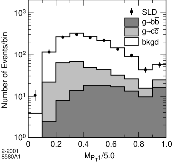
Figure 1: Distribution of $M_{P_{T}1}$ (see text). The right-most bin includes overflows. The points represent the data, the histogram the simulation; the expected contribution from $g$ $\rightarrow$$b\bar{b}$   ($g$ $\rightarrow$${c}\bar{c}$ ) (see text) is shown as the dark (shaded) area.

1. $M_{P_{T}1}$: $b$ jets typically have higher values of this quantity than $c$ or $uds$ jets. The distribution of $M_{P_{T}1}$ is shown in Figure 1.

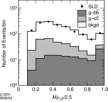
Figure 2: Distribution of $M_{P_{T}2}$ (see text). The right-most bin includes overflows. The points represent the data, the histogram the simulation; the expected contribution from $g$ $\rightarrow$$b\bar{b}$   ($g$ $\rightarrow$${c}\bar{c}$ ) (see text) is shown as the dark (shaded) area.

2. $M_{P_{T}2}$: This observable has similar discriminating power. The distribution of $M_{P_{T}2}$ is shown in Figure 2.

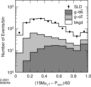
Figure 3: Distribution of $15M_{P_{T}1}-P_{vtx1}$ (see text). The right-most bin includes overflows. The points represent the data, the histogram the simulation; the expected contribution from $g$ $\rightarrow$$b\bar{b}$   ($g$ $\rightarrow$${c}\bar{c}$ ) (see text) is shown as the dark (shaded) area.

3. $15M_{P_{T}1}-P_{vtx1}$: where $P_{vtx}$ is the vertex momentum. This observable tends to be large for $b$ jets since $B$ decay vertices typically have higher mass than those from charm decays, and vertices resulting from $B$ $\rightarrow$$D$ cascade decays have a lower momentum than those from primary $D$ hadrons. The distribution of $15M_{P_{T}1}-P_{vtx1}$ is shown in Figure 3.

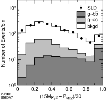
Figure 4: Distribution of $15M_{P_{T}2}-P_{vtx2}$ (see text). The right-most bin includes overflows. The points represent the data, the histogram the simulation; the expected contribution from $g$ $\rightarrow$$b\bar{b}$   ($g$ $\rightarrow$${c}\bar{c}$ ) (see text) is shown as the dark (shaded) area.

4. $15M_{P_{T}2}-P_{vtx2}$: This observable also has discriminating power between signal and background events. The distribution of $15M_{P_{T}2}-P_{vtx2}$ is shown in Figure 4.

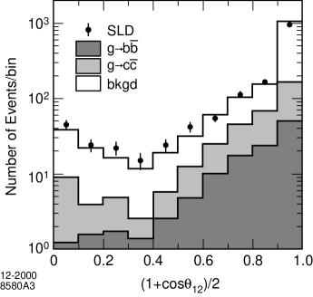
Figure 5: Distribution of cos$\theta_{12}$ (see text). The points represent the data, the histogram the simulation; the expected contribution from $g$ $\rightarrow$$b\bar{b}$   ($g$ $\rightarrow$${c}\bar{c}$ ) (see text) is shown as the dark (shaded) area.

5. The angle $\theta_{12}$ between the vertex axes of jets 1 and 2. The two jets from $g$ $\rightarrow$$b\bar{b}$ tend to have $\theta_{12}$ $\simeq 0$. However, in some $Z^{0}$ $\rightarrow$$b\bar{b}$ background events a single $b$ jet may be split into two by the jet-finder; in these cases the two reconstructed vertices tend to have $\cos\theta_{12}\geq 0.98$. The distribution of cos$\theta_{12}$ is shown in Figure 5.

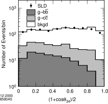
Figure 6: Distribution of cos$\theta_{34}$ (see text). The points represent the data, the histogram the simulation; the expected contribution from $g$ $\rightarrow$$b\bar{b}$   ($g$ $\rightarrow$${c}\bar{c}$ ) (see text) is shown as the dark (shaded) area.

6. The angle $\theta_{34}$ between the axes of jets 3 and 4. In events containing $g$ $\rightarrow$$b\bar{b}$ this tends to be near $\pi$, while background events tend to populate the smaller-angle region. The distribution of cos$\theta_{34}$ is shown in Figure 6.

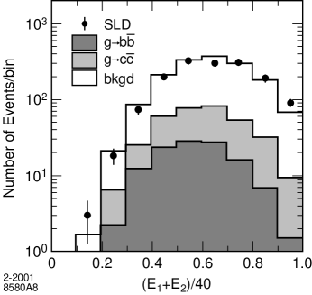
Figure 7: The distribution of the energy sum of jets 1 and 2. The points represent the data, the histogram the simulation; the expected contribution from $g$ $\rightarrow$$b\bar{b}$   ($g$ $\rightarrow$${c}\bar{c}$ ) (see text) is shown as the dark (shaded) area.

7. The energy sum of jets 1 and 2, $E_{1}+E_{2}$: The two jets arising from $g$ $\rightarrow$$b\bar{b}$ tend to have lower energy than the other two jets in the event. The distribution of $E_{1}+E_{2}$ is shown in Figure 7.

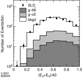
Figure 8: The distribution of the energy sum of jets 3 and 4. The points represent the data, the histogram the simulation; the expected contribution from $g$ $\rightarrow$$b\bar{b}$   ($g$ $\rightarrow$${c}\bar{c}$ ) (see text) is shown as the dark (shaded) area.

8. The energy sum of jets 3 and 4, $E_{3}+E_{4}$: This tends to be larger in signal events than in background events. The distribution of $E_{3}+E_{4}$ is shown in Figure 8.

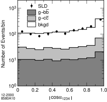
Figure 9: The distribution of $\cos\alpha_{1234}$ (see text). The points represent the data, the histogram the simulation; the expected contribution from $g$ $\rightarrow$$b\bar{b}$   ($g$ $\rightarrow$${c}\bar{c}$ ) (see text) is shown as the dark (shaded) area.

9. The angle $\alpha_{1234}$ between the plane $\Pi_{12}$ formed by jets 1 and 2 and the plane $\Pi_{34}$ formed by jets 3 and 4: This variable is similar to the Bengtsson-Zerwas angle [19], and is useful to separate $g$ $\rightarrow$$b\bar{b}$ events because the radiated virtual gluon in the process $Z^{0}$ $\rightarrow$$q\overline{q}g$ is polarized in the three-parton plane, and this is reflected in its subsequent splitting, by favoring $g$ $\rightarrow$$q\overline{q}$ emission out of this plane, i.e.$\alpha_{1234}\simeq\pi/2$. The distribution of cos$\alpha_{1234}$ [20] is shown in Figure 9.

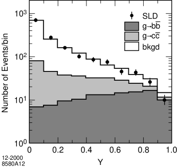
Figure 10: Distribution of the neural network output $Y$. The points represent the data, the histogram the simulation; the expected contribution from $g$ $\rightarrow$$b\bar{b}$   ($g$ $\rightarrow$${c}\bar{c}$ ) (see text) is shown as the dark (shaded) area.

The measured and simulated distributions agree well for these input observables. We trained the neural network using Monte-Carlo samples of about 1800k $Z^{0}$ $\rightarrow$$q\overline{q}$ events, 1200k $Z^{0}$ $\rightarrow$$b\bar{b}$ events, 780k $Z^{0}$ $\rightarrow$${c}\bar{c}$ events and 50k events containing $g$ $\rightarrow$$b\bar{b}$ . These samples were independent of the ones used for the selection efficiency and background studies. Figure 10 shows the distribution of the neural network output variable, $Y$. We retained events with $Y$ greater than 0.7. This value was found to minimise the total error on the final $g_{b\bar{b}}$ result.

5 Result

79 events were selected in the data. The number of background events was estimated, using the Monte Carlo simulation, to be $41.9$, where $35\%$ of the background comes from $g$ $\rightarrow$${c}\bar{c}$ events, $63\%$ from $Z^{0}$ $\rightarrow$$b\bar{b}$ events, and the remaining $2\%$ from $Z^{0}$ $\rightarrow$$q\overline{q}$ $(q\neq b)$ events. Table 1 shows the selection efficiencies, relative to the selected hadronic-event sample, for the B, C and Q event categories. From these efficiencies and the fraction of events selected in the data, $f_{d}=(2.73\pm 0.31)\times 10^{-4}$, the value of $g_{b\bar{b}}$ was determined:

$$g_{b\bar{b}}=\frac{f_{d}-(1-g_{c\bar{c}})\epsilon_{Q}-g_{c\bar{c}}\epsilon_{C}}{\epsilon_{B}-\epsilon_{Q}}.$$ (1)

We obtained

$$g_{b\bar{b}}=(2.44\pm 0.59)\times 10^{-3},$$ (2)

where the error is statistical only.

Source Efficiency ($\%$) B $5.28\pm 0.09$ ($\epsilon_{B}$) C $0.165\pm 0.018$ ($\epsilon_{C}$) Q $0.00967\pm 0.00038$ ($\epsilon_{Q}$)

Table 1: Selection efficiencies after all cuts for the three categories. Errors are statistical only.

6 Systematic Errors

The efficiencies for the three event categories were evaluated using the Monte-Carlo simulation. The limitations of the simulation in estimating these efficiencies lead to an uncertainty on the result. The error due to limited Monte-Carlo statistics in the efficiency evaluation was $\Delta g_{b\bar{b}}=\pm 0.12\times 10^{-3}$.

A large fraction of events remaining after the selection cuts contain $B$ and $D$ hadrons. The uncertainty in the knowledge of the physical processes in the simulation of heavy-flavor production and decays constitutes a source of systematic error. All the physical simulation parameters were varied within their allowed experimental ranges. In particular, the $B$ and $D$ hadron lifetimes, their production rates, and the mean $B$ hadron energy were varied following the recommendations of the LEP Heavy Flavour Working Group [21]. We also varied the assumed form of the $B$ energy distribution, taking the difference between the optimised Bowler and Peterson functions [22] to assign an error. The uncertainties, which are typically small, are summarized in Table 2.

Source $\Delta g_{b\bar{b}}$ $(10^{-3})$ Monte Carlo statistics $\pm 0.12$ $B$ hadron lifetimes $\pm 0.01$ $B$ hadron production $\pm 0.02$ Mean $B$ hadron energy $\pm 0.10$ $B$ fragmentation function $\pm 0.09$ $B$ hadron charged multiplicities $\pm 0.03$ $B\to DDX$ fraction $\pm 0.07$ $D$ hadron lifetimes $\pm 0.01$ $D$ hadron production $\pm 0.02$ $D$ hadron charged multiplicities $\pm 0.02$ Theoretical modelling of $g$ $\rightarrow$$b\bar{b}$ kinematics $\pm 0.24$ $b$ quark mass $\pm 0.05$ $g_{c\bar{c}}$ $\pm 0.12$ Tracking efficiency $\pm 0.04$ Total $\pm 0.34$

Table 2: Systematic uncertainties on $g_{b\bar{b}}$.

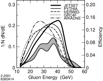
Figure 11: Energy distribution (left-hand scale) of gluons for the $g$ $\rightarrow$$b\bar{b}$ process in different models (see text). Our calculated efficiency and its uncertainty (see text) are shown as the band (right-hand scale).

The dominant systematic error arises via the signal tagging efficiency, $\epsilon_{B}$, from the dependence on modelling the kinematics of the split gluon: its energy $E_{g}$, its mass $m_{g}$ and the decay angle, $\theta^{*}$, of the two $B$ hadrons in their center-of-mass frame relative to the gluon direction. In our default Monte Carlo simulation the kinematics of the signal events are based on the JETSET parton shower, which is in good agreement with the theoretical predictions [2]. In order to estimate the uncertainty on this assumption, we have investigated alternative models, namely the PYTHIA 6.136, HERWIG 6.1 [23], and ARIADNE 4.08 [24] models, as well as the exact leading-order matrix-element calculation GRC4F [25]. In each case, we generated, at the parton level, events containing $g$ $\rightarrow$$b\bar{b}$ . For illustration the $E_{g}$ distributions are shown in Fig. 11. The efficiency function computed with JETSET was then reweighted by the ratio of the new model to JETSET initial distributions to obtain a new estimate of the average efficiency. The resulting $g_{b\bar{b}}$ values are shown in Table 3. We took the central value of this ensemble, $g_{b\bar{b}}$ = 2.44 $\times 10^{-3}$, as our central result, and assigned a systematic error of $\Delta g_{b\bar{b}}=\pm 0.24\times 10^{-3}$ based on the full range of values. For illustration the efficiency and its uncertainty are shown in Fig. 11.

Model $g_{b\bar{b}}$ ($\times 10^{-3}$) JETSET 7.4 2.20 PYTHIA 6.136 2.22 HERWIG 6.1 2.50 ARIADNE 4.08 2.41 GRC4F 2.68

Table 3: $g_{b\bar{b}}$ values resulting from different models of the gluon kinematics.

The dependence of the efficiency on the $b$-quark mass was also investigated at the generator level using the GRC4F Monte Carlo program. The variation of $\epsilon_{B}$ was computed for $b$-quark masses between $4.7$ and $5.3$ GeV/c². The resultant uncertainty is estimated to be $\Delta g_{b\bar{b}}=\pm 0.05\times 10^{-3}$. The measured uncertainty in the production fraction of $g$ $\rightarrow$${c}\bar{c}$ background events, $\Delta g_{c\bar{c}}=\pm 0.40{\rm\%}$, gives an error $\Delta g_{b\bar{b}}=\pm 0.12\times 10^{-3}$.

In the Monte-Carlo simulation charged tracks used in the topological vertex tag were rejected to reproduce better the distributions in the data. Uncertainties in the efficiencies due to this rejection were assessed by evaluating the Monte-Carlo efficiencies without the rejection algorithm. The difference in the $g_{b\bar{b}}$ result was taken as a symmetric systematic error, $\Delta g_{b\bar{b}}=\pm 0.04\times 10^{-3}$.

As cross checks we varied independently the value of $y_{cut}$ used in the 4-jet event selection and the value of the neural network output, $Y$, used to select the final event sample. In each case we found results consistent with those determined using the optimised value. Table 2 summarizes the different sources of systematic error on $g_{b\bar{b}}$. The total systematic error was estimated to be the sum in quadrature, $0.34\times 10^{-3}$.

7 Summary

Using the excellent flavor-tagging capabilities of the SLD tracking system, and a new technique incorporating a multivariate neural network analysis, we have measured the probability for gluon splitting into $b\bar{b}$ in hadronic $Z^{0}$ decays. The result is

$$g_{b\bar{b}}=(2.44\pm 0.59{\rm(stat.)}\pm 0.34{\rm(syst.)})\times 10^{-3}$$

where the first error is statistical and the second is the sum in quadrature of systematic effects. This represents the most precise determination of $g_{b\bar{b}}$ to date. Our result is consistent with previous measurements [3]. It is also consistent with the theoretical expectation $g_{b\bar{b}}$ = $1.75\pm 0.40\times 10^{-3}$ [2], where the central value corresponds to $\alpha_{s}(M_{Z}^{2})$= 0.118 and a $b$-quark mass of 5.0 GeV/$c^{2}$. Finally, we found that the predictions of the models PYTHIA6.136 ($g_{b\bar{b}}$ = $1.5\times 10^{-3}$) and HERWIG6.1 ($g_{b\bar{b}}$ = $2.5\times 10^{-3}$), with their default parameter settings, are consistent with our measurement. The prediction of ARIADNE4.08 ($g_{b\bar{b}}$ = $1.3\times 10^{-3}$) is slightly below our measurement.

References

- [1] In this analysis we do not distinguish between quark and antiquark jets.
- [2] D.J. Miller and M.H. Seymour, Phys. Lett. B435 213 (1998).
-
[3]
ALEPH Collab., R. Barate et al., Phys. Lett. B434 437 (1998);
DELPHI Collab., P. Abreu et al., Phys. Lett. B462 425 (1999);
OPAL Collab., G. Abbiendi et al., CERN-EP/2000-123; subm. to Eur. Phys. J. C. -
[4]
ALEPH Collab., R. Barate et al., Phys. Lett. B401 150 (1997);
ALEPH Collab., R. Barate et al., Phys. Lett. B401, 163 (1997);
DELPHI Collab., P. Abreu et al. Z. Phys. C70, 531 (1996);
L3 Collab., O. Adriani et al., Phys. Lett. B307, 237 (1993);
OPAL Collab., G. Abbiendi et al., Eur. Phys. J. C8, 217 (1999);
SLD Collab., K. Abe et al., Phys. Rev. Lett. 80, 660 (1998). - [5] SLD Design Report, SLAC Report 273 (1984).
- [6] SLD Collab., K. Abe et al., Phys. Rev. D56 (1997) 5310.
- [7] M.D. Hildreth et al., IEEE Trans. Nucl. Sci. 42 (1994) 451.
- [8] SLD Collab., K. Abe et al., Nucl. Inst. Meth. A400, (1997) 287.
- [9] SLD Collab., K. Abe et al., Phys. Rev. D53 (1996) 1023.
- [10] T. Sjostrand, Comput. Phys. Commun. 82, 74 (1994).
-
[11]
P. N. Burrows, Z. Phys. C41 375 (1988).
OPAL Collab., M.Z. Akrawy et al., Z. Phys. C47 505 (1990). - [12] SLD Collab., K. Abe et al., Phys. Rev. Lett.79 590 (1997).
- [13] R. Brun et al., Report No. CERN-DD/EE/84-1 (1989).
- [14] SLD Collaboration, K. Abe et al., Phys. Rev. D51, 962 (1995).
-
[15]
ALEPH Collab., R. Barate et al., Eur. Phys. J. C16 597 (2000);
L3 Collab., M. Acciarri et al., Phys. Lett. B476 243 (2000);
OPAL Collab., G. Abbiendi et al., Eur. Phys. J. C13 1 (2000). - [16] S. Schmitt, Proc. International Europhysics Conference on High Energy Physics, Tampere, Finland, July 15-21, 1999, p. 645.
- [17] D.J. Jackson, Nucl. Instrum. Meth. A388, 247 (1997).
- [18] S. Catani, Y.L. Dokshitzer, M. Olsson, G. Turnock and B.R. Webber, Phys. Lett. B269, 432 (1991).
- [19] M. Bengtsson and P.M. Zerwas, Phys. Lett. B208, 306 (1988).
- [20] The peak at 1 in the distribution of is an artefact of the mapping from the distribution of .
- [21] The LEP Heavy Flavour Working Group, LEPHF/98-01.
- [22] SLD Collab., Kenji Abe et al., Phys. Rev. Lett. 84 (2000) 4300.
-
[23]
G. Marchesini et al., Comput. Phys. Commun. 67 465 (1992);
G. Corcella et al., hep-ph/9912396. - [24] L. Lönnblad, Comput. Phys. Commun. 71 15 (1992); we used the kinematic cut MSTA(28)=1.
- [25] J. Fujimoto et al., Comput. Phys. Commun. 100, 128 (1997).