DELPHI 2000-069 PHYS 868 IEKP-KA/2001-3
BSAURUS- A Package For Inclusive B-Reconstruction in DELPHI.
Z. Albrecht, T. Allmendinger, G. Barker
M. Feindt, C. Haag, M. Moch.
University of Karlsruhe
BSAURUS is a software package for the inclusive reconstruction of B-hadrons in events taken by the DELPHI detector. The BSAURUS goal is to reconstruct B-decays, by making use of as many properties of b-jets as possible, with high efficiency and good purity. This is achieved by exploiting the capabilities of the DELPHI detector to their extreme, applying wherever possible physics knowledge about B production and decays and combining different information sources with modern tools- mainly artificial neural networks. This note provides a reference of how BSAURUS outputs are formed, how to access them within the DELPHI framework, and the physics performance one can expect.
1 Introduction
BSAURUS is a package for inclusive B reconstruction of decays into b quark-antiquark pairs taken by the DELPHI detector. Due to the large mass of B hadrons there are many thousand decay channels, all with small branching ratio. This is a severe limitation for studying B physics. BSAURUS tries to reconstruct inclusively as many properties of b-jets as possible with high efficiency and yet with good purity also. This is achieved by exploiting the capabilities of the DELPHI detector to their extreme, applying wherever possible physics knowledge about B production and decays and combining different information sources with modern tools- mainly artificial neural networks.
1.1 Physics Motivation
High energy b-jets contain ,, mesons or B-baryons in an approximate mixture of 40:40:10:10. To measure lifetimes one needs to be able to reconstruct the decay length, i.e. the distance between primary and secondary vertex, as well as the B-hadron energy. The mean lifetime of B-hadrons have been measured with good accuracy and together with the semileptonic branching ratio it can be used to determine the Cabibbo-Kobayashi-Maskawa matrix element . The lifetimes of the individual B hadrons are predicted by the Heavy Quark Effective Theory (HQET) to be only marginally different from the mean lifetime. In order to test HQET, one needs to be able to distinguish between the four B hadron species.
The fraction of the available energy that B-hadrons attain after the fragmentation process is not directly calculable in perturbative QCD, and has to be phenomenologically modelled with fragmentation functions. Measuring the b-quark fragmentation function, ideally for the different B-types separately, is fundamental to the accurate simulation of B-physics.
The decay into b-quarks exhibits a forward-backward asymmetry between the b and -jet. A precise measurement of constitutes an important test of the Standard Model. For an experimental study one needs to tag the production flavour (i.e. decide whether a given jet is from a b-quark or antiquark). Neutral B mesons can oscillate into their antiparticle (and back) before they decay. The time dependence of oscillations has been observed, whereas the oscillations of the meson are too fast to be experimentally resolved at present . For experimental studies of -oscillations one needs to know the production flavour and the decay flavour.
The weakly decaying B hadrons are the lowest mass, i.e. the ground states, of systems with quantum numbers . For each of these systems a full spectroscopy of excited states exists, e.g. vector mesons and orbital excitations which are predicted to appear as two doublets for each unit of orbital angular momentum L, one being broad decaying in S-wave, and the other narrow since at least D-waves are necessary in the decay. Signals of B-mesons are observed with a relatively large rate (about 20-30%), but the composition of the broad peak observed is still unclear. Radial excitations are also predicted in the quark model. In B-baryon spectroscopy, in addition to the , the states , and are expected to decay via weak interactions with an appreciable lifetime, whereas the and should decay into via strong interactions. For testing B-spectroscopy one needs the reconstruction of B-hadron four-momenta and the identification of protons, pions and kaons originating from the fragmentation process.
BSAURUS is designed primarily to allow analyses in all these areas. The algorithms used rely on a satisfactory performance from all of the detector components in the DELPHI barrel in conjunction with optimised reconstruction software.
1.2 Detector-Specific Reconstruction: The Basis of BSAURUS
Charged particle reconstruction, especially the correct assignment of silicon vertex detector points to tracks reconstructed in the TPC, the Inner Detector and the Outer Detector, has been optimised in the years 1995/1996 by better alignment procedures and adding completely new algorithms including e.g. inside-out tracking, a complete event ambiguity resolution, and a Kalman filter track fit taking into account multiple scattering and energy loss. All LEP I data taken from 1992-1995 have been reprocessed with these new algorithms, and this has led to huge reconstruction improvements, especially in dense jets. As an example, the signal of exclusively reconstructed mesons into with was increased by a factor 2.4. In addition, optimised photon conversion algorithms [1], reconstruction of secondary hadronic interactions in detector material and of decays, and a search for additional low-energy tracks in the vertex detector [2] help to give a clean reconstruction of complicated events. It should be noted that since BSAURUS has been developed and tuned on these reprocessed data the result of applying it to any other data set cannot be guaranteed.
Particle identification is an important ingredient for many of the algorithms applied. To achieve an optimal performance, electron identification [1] is performed using a neural network combining spatial and energy information from the HPC calorimeter, tracking information, dE/dx measurements of the TPC, and searches for kinks in the track in known layers of material and for photons radiated tangentially in them. In DELPHI, hadron identification information is gathered from the Ring Imaging Cerenkov Counters(RICH) with both gas and liquid radiator, and from energy loss measurements in the TPC and the silicon vertex detector. To optimise hadron classification at various momenta, detailed information from all of these detectors has been combined using neural networks in the program package MACRIB [3].
1.3 Overview Of BSAURUS Outputs
BSAURUS provides a host of information relating to the properties of B-hadron production, fragmentation and decay within an event hemisphere. This information is available via output variables stored in COMMON blocks, described in Appendix C.
Among the most important outputs for B-physics analysis topics are:
- •
-
•
the TrackNet (see Section 5) that discriminates between tracks originating from the primary and a secondary vertex,
-
•
the BDnet (see Section 7) that discriminates between tracks originating from the B and the cascade BD vertex,
-
•
neural networks (see Section 6) that provide a probability that a particular B-hadron type (i.e. or B-baryon) was present in the hemisphere,
-
•
neural networks (see Section 8) that tag the charge or flavour of the b-quark in the B-hadron type at both the production and decay time.
2 BSAURUS Definitions
2.1 Multihadronic Events
There is no event selection applied inside BSAURUS i.e. it is left to the user to decide on which events to call BSAURUS. However, for all development and tuning work and for all results presented in this note, events in real data and Monte Carlo had to pass a multihadronic event selection. The criteria used are from the DELPHI pilot record hadron selection bits:
-
•
team 4 selection, charged particles (bit 1)
-
•
team 4 selection, charged energy (bit 2)
-
•
, (bit 12).
2.2 Standard Particle Selection
Charged particles used by the BSAURUS algorithms must pass the following track selection criteria:
-
•
Impact parameter, with respect to the origin, in the plane cm
-
•
Impact parameter, with respect to the origin, in the plane cm
-
•
-
•
-
•
At least 1 track hit from the silicon vertex detector(VD)
-
•
Tracks must not have been flagged as originating from material interactions (via any of the PXPHOT codes: -124, -123, -75, -85, -84 or -74).
Neutral particles are used that are flagged by the DELPHI mass code as being a photon, , or (codes 21, 47, 61 and 81 respectively).
2.3 Event Jets
Event jets are reconstructed via the routine LUCLUS [4]. All reconstructed particles, that pass the standard selection, are used with a transverse momentum cutoff value of =PARU(44)=5.0.
2.4 Event Hemispheres
All reconstructed particles, that pass the standard selection, are used to calculate the event thrust axis via routine LUTHRU [4]. Event hemispheres are then defined by the plane perpendicular to the thrust axis.
Each hemisphere has associated with it two axes: the thrust axis and the reference axis used for the calculation of rapidity (see Section 2.5 below) for tracks in that hemisphere. The reference axis is a jet axis selected in the following way:
-
•
If the event is a two jet event, the reference axis for the hemisphere is the jet axis in that hemisphere.
-
•
If a hemisphere contains 2 or more jets (i.e. an event with 3 or more jets) :
-
–
if one of the jets is the highest energy jet in the event, that jet axis forms the reference axis.
-
–
if the highest energy jet is in the opposite hemisphere, the combined probability () for the tracks in a jet to have originated from the event primary vertex is formed (via the AABTAG package algorithms[5]).
The jet that is most ‘B-like’, i.e. with the smallest probability, is then selected if .
-
–
if no jet in the hemisphere satisfies the above criteria, the jet with the highest energy is selected to form the reference axis.
-
–
In addition, internally to BSAURUS, the hemispheres are numbered as 1 or 2 with the convention that the jet forming the reference axis for hemisphere 1 is of higher energy than that for hemisphere 2.
2.5 Track Rapidity
The rapidity of a track is defined as follows,
for the track energy and the longitudinal momentum component along the reference axis for the hemisphere.
The BSAURUS rapidity algorithm also returns an initial estimate of the B-hadron candidate 4-vector. This is defined simply to be the sum of individual track momentum vectors in a hemisphere for tracks with rapidity greater than 1.6. The value of the cut provides a good rejection of tracks originating from the primary vertex while accepting the majority of tracks from the B-decay.
2.6 Particle Identification
Unless otherwise stated, particle identification in BSAURUS is based on the following definitions:
-
•
Charged kaons: the kaon network output, or kaon probability, from the MACRIB package [3] and stored in BSAURUS output
BSPAR(IBP_MACK,IH). -
•
Protons: the proton network output, or proton probability, from the MACRIB package [3]and stored in BSAURUS output
BSPAR(IBP_MACP,IH). -
•
Electrons: the electron network output, or electron probability, returned by the ELEPHANT routine
ELNETID[1]. -
•
Muons: the
MUCAL2definitions of a very loose, loose, standard and tight muon.
2.7 Performance of Networks
The main tool used to quantify and compare BSAURUS network performance is the purity against efficiency plot. Given some definition of ‘signal’ and ‘background’, purity is defined as,
| (1) |
and the efficiency defined as,
| (2) |
In this note, the efficiency is calculated after all selection cuts, e.g. from Section 2.2 and Section 4, have been applied. When considering network outputs that involve symmetric binary decisions (i.e. the TrackNet and all flavour tagging networks), we use an alternative measure of efficiency termed ‘fraction classified’ and defined as,
| (3) |
For this case, in order to make the purity-efficiency plot, is varied by making successive cuts in a band around the equal probability point for tagging ‘signal’ or ‘background’.
3 General BSAURUS Quantities
3.1 Secondary Vertex Finding
Per-hemisphere, an attempt is made to fit a secondary vertex to tracks with rapidity that pass the standard track selection criteria of Section 2.2.
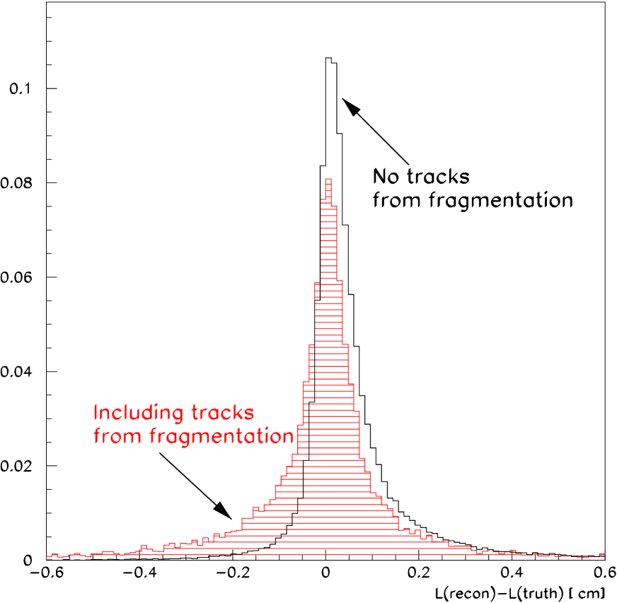
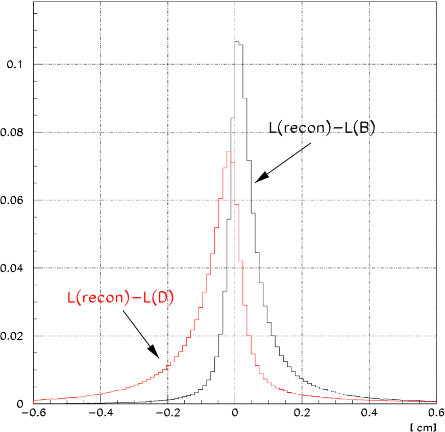
From this class of track, additional criteria are applied with the aim of selecting tracks for the vertex fitting stage that are likely to have originated from the decay chain of a weakly decaying B-hadron state. As Figure 1 illustrates, it is important to reject as far as possible tracks from the fragmentation in order to avoid large pulls in the vertex position toward the primary vertex.
There must be a minimum of two tracks for the vertex fit to be attempted and the selection process is as follows:
-
[1]
The highest energy muon or electron candidate is selected if GeV.
-
[2]
The crossing point of each track with the initial B-candidate direction vector (see Section 2.5) is found and the distance, , between primary vertex 111Unless otherwise stated, the primary vertex definition in BSAURUS is the event primary vertex from the AABTAG package. and crossing point is calculated. Tracks are selected if or, for cases where , tracks must also satisfy and cm.
If at this point the number of tracks selected for the fit is less than 2, further attempts are made to add tracks to the fitting procedure. When this happens in events, it is likely that the true decay length of the B-hadron was small.
If only one track was added from stages 1 and 2:
-
[3]
Add tracks with .
-
[4]
If still only one track selected, add the track of highest rapidity from the remaining track list of the hemisphere.
If no track was selected from stages 1) and 2):
-
[5]
A search is made for the best kaon candidate in the hemisphere based on the kaon probability defined in Section 2.6. If this kaon candidate has it is added to that track in the remaining track list of the hemisphere that has the highest rapidity. This track pair alone will then form the starting track list for the vertexing procedure.
-
[6]
Finally if no kaon candidate exists in the hemisphere, the two tracks of highest rapidity are selected.
Using the track list supplied by this track selection process, a secondary vertex fit is performed in 3-dimensions (using routine DAPLCON from the ELEPHANT package [1]) constrained to the direction of the B-candidate momentum vector. The event primary vertex is used as a starting point and if the fit did not converge222Here, non-convergence means the fit took more than 20 iterations. A further iteration is deemed necessary if the is above 4 standard deviations during the first 10 iterations or above 3 standard deviations during the next 10 iterations., the track making the largest contribution is stripped away in an iterative procedure, and the fit repeated.
In addition to returning the secondary vertex position, the procedure also fits the primary vertex position and updates the B-candidate direction according to the vector joining the primary and secondary vertex points. This information is used in forming some of the track net inputs as described in the next section.
Once a convergent fit has been attained, the final stage of the secondary vertex fitting procedure involves an attempt to add into the fit tracks that failed the initial track selection criteria but nevertheless are consistent with originating from the vertex. These tracks are identified on the basis of an intermediate version of the TrackNet. This is a neural network output that discriminates between tracks originating from the primary vertex and those likely to have come from a secondary vertex and is described in Section 5. A version of the TrackNet is constructed, specifically for the purpose of use in this final stage of vertex fitting, based on secondary vertexing information available before this final stage has run. In general, secondary vertex tracks have TrackNet whereas tracks from the primary vertex have TrackNet values close to zero. The track of largest TrackNet in the hemisphere is added to the existing track list and retained if the resulting fit converges. This process continues iteratively for all such tracks with TrackNet .
3.2 B-Candidate Four-Vectors Available from BSAURUS
BSAURUS provides currently four different definitions of the B-candidate four-vector in a hemisphere:
-
•
The initial estimate from the rapidity algorithm outlined in Section 2.5 and stored in the four BSAURUS output array elements starting at
BSHEM(IBH_BY,IH)for hemisphere numberIH. -
•
The three momentum vector is then transformed to lie along the direction joining primary to secondary vertex as mentioned in Section 3.1. The energy component is the rapidity energy and this vector is stored in location starting at
BSHEM(IBH_BF,IH). -
•
In location starting at
BSHEM(IBH_BT,IH), the energy component is then corrected to account for neutral energy losses (see Section 3.3). The momentum vector derives from a TrackNet weighted momentum sum for the case of 2-jet events and is the rapidity vector for -jet events. -
•
The four-vector starting at location
BSHEM(IBH_BTT,IH)is, in principle, the same as theBSHEM(IBH_BT,IH)vector but contains a more detailed energy correction, described in detail in Section 3.3. In addition, the momentum vector derives from the rapidity algorithm for -jet events that also pass and from the TrackNet weighted sum otherwise.
3.3 B-Candidate Energy Correction
We describe here the energy correction procedure that went into making vector
BSHEM(IBH_BTT,IH). (Note that the BSHEM(IBH_BT,IH) vector
contains a very similar correction which, although still used internally
inside BSAURUS, is older and less optimal.)
Separate correction functions are derived for 2-jet and -jet events. Within these two classes, because of the explicit energy ordering of the hemispheres, we treat hemispheres 1 and 2 completely separately. To be used in the correction procedure, hemispheres must pass the following cuts:
-
•
The initial reconstructed B-candidate energy is 20GeV or more.
-
•
The corresponding initial reconstructed B-candidate mass lies within two standard deviations of the total data sample median value.
-
•
The ratio, , of the hemisphere energy to beam energy lies in the range .
In addition, for the case of hemispheres with larger missing energy, i.e. , a further correction is derived separately for hemispheres 1 and 2.
The starting point is the initial estimates of the B energy and mass, and . Following studies, we choose these estimates to be from the rapidity algorithm for events with -jets and where , and to be derived from the sum of ‘B-weighted’ four-vectors otherwise. This involves weighting (via a sigmoid threshold function) the momentum and energy components of charged tracks by the TrackNet output (see section 5) and those of neutrals by their rapidity. In this way the effects of tracks from the B-decay are enhanced and those of tracks from the primary vertex are suppressed.
The correction procedure is motivated by the observation in Monte Carlo of a correlation between the energy residuals and (which is approximately linear in ), and a further correlation between and resulting from neutral energy losses and inefficiencies. The correction proceeds in the following way: the data are divided into several samples according to the measured ratio and for each of these classes the B-energy residual is plotted as function of . The median values of in each bin of are calculated and their dependence fitted by a third order polynomial
The four parameters in each class are then plotted as a function of and their dependence fitted with third and second-order polynomials. Thus one obtains a smooth correction function describing the mean dependence on and on the hemisphere energy as determined from the Monte Carlo. Finally, a small bias correction is applied for the remaining mean energy residual as a function of the corrected energy.
Figure 2 shows typical resolutions on the reconstructed
B-direction and energy attainable from the four-vector
output at location BSHEM(IBH_BTT,IHEM).

3.4 Decay Length and Decay Time
The B-hadron decay length estimate in the plane, , is defined as the (positive) distance between the primary and secondary vertex positions reconstructed from the secondary vertex search described in Section 3.1. The three-dimensional decay length is constructed as , where the B-hadron candidate momentum vector, detailed in Section 3.3, defines the direction. The resulting proper decay time estimate is given by , where the B rest mass is taken to be GeV.
3.5 Track and Hemisphere Quality
When presenting neural networks with track and hemisphere-based discriminating variables, it is advantageous at the network learning stage to provide the network with additional information relating to the potential quality of the input information. For this reason BSAURUS defines both track and hemisphere quality words that are used extensively in many network definitions.
The track quality word stored in BSPAR(IBP_QUAL,IT) for track IT
is defined as follows:
-
•
0, means the track is good.
-
•
1, means the track contains some ambiguous track hit information flagged by the DELPHI track hit ambiguity word.
-
•
10, means that the track has been flagged as originating from an interaction, defined by PXPHOT code=-120 returned by routine PXGECO.
-
•
20, means that the track did not pass the internal track quality criteria of the AABTAG package.
The hemisphere quality word, stored in, BSHEM(IBH_QUAL,IH) for hemisphere
IH, has the following definition:
-
•
, where is the number of tracks in the hemisphere rejected by the standard track cuts (described in Section 2.2)
-
•
+ , where is the number of tracks in the hemisphere flagged as originating from an interaction in the same way as for the track quality word
-
•
+ , where is the number of tracks in the hemisphere flagged as being ambiguous in the same way as for the track quality word
-
•
+ , where is the number of tracks in the hemisphere flagged as failing the quality cuts of the AABTAG package.
For use in network training, the hemisphere quality is better used in
a real, continuous form rather than as an integer. Stored in BSHEM(IBH_QUAL2,IH)
therefore, is the transformation of the integer word into a
continuous variable ranging from 0.0(good quality) to 10.0(bad quality).
4 Use of Neural Networks in BSAURUS
Events and event hemispheres used to prepare the training samples for BSAURUS networks must pass the following set of requirements:
-
•
2-jet events with the jets back-to-back to better than ,
-
•
,
-
•
combined AABTAG event b-tag ,
-
•
both gas and liquid parts of the RICH must be functioning,
-
•
defining as the total energy contained in charged and neutral particles in the hemisphere, then a hemisphere must satisfy ,
-
•
a hemisphere must have an initial B-energy estimate from the rapidity algorithm GeV,
-
•
only hemispheres with a fully converged secondary vertex fit are considered.
BSAURUS uses the JETNET[6] neural network package run in a feed-forward mode nearly always with three layers and a sigmoid function as the input-output(or transfer) function. The hidden layer typically contains one more node than the number of inputs.
The network is trained using two statistically independent samples; the training sample and the performance sample. Usually each sample consists of an equal number of ‘signal’ and ‘background’ hemispheres/tracks. The training sample is used to teach the network to separate signal from background, but it is the network output error333Defined as , where index labels the network output node, is the network output value at output node and is the target value for output node . based on the performance sample that determines when the end-point of the training procedure has been reached.
Variables used as inputs to the networks are selected based on (a)the discriminating power between signal and background and (b)the agreement between simulation and data. Variables are often also transformed and/or their range truncated so that the network is presented with variables that show, ideally, a linear, continuous variation in the ratio of ‘signal’ to ‘background’ across the full range.
5 The B-Track Probability Network(TrackNet)
The aim of the B-track probability network is to discriminate between the class of tracks, in a -event hemisphere, originating from the weak decay of a B-hadron from all other tracks.
Only tracks passing the standard quality cuts of Section 2.2 are considered. The discriminating variables that form the inputs to the network per track are:
-
•
The track total momentum.
-
•
The track momentum in the B-candidate rest frame.
-
•
The helicity angle of the track defined as the angle between the track vector in the B-candidate rest frame and the B-candidate momentum vector in the lab frame.
-
•
A flag to identify whether the track was in the secondary vertex fit or not.
-
•
The probability that the track originates from the fitted primary vertex (AABTAG algorithm).
-
•
The probability that the track originates from the secondary vertex (AABTAG algorithm).
-
•
The probability that the track originates from the fitted primary vertex (BSAURUS algorithm).
-
•
The probability that the track originates from the secondary vertex (from the BSAURUS algorithm).
-
•
The track rapidity.
In addition, input variables that gave no inherent discriminating power were included to inform the network of the potential quality of the other input variables:
-
•
The decay length or distance between the primary and secondary vertex in the plane. This quantity is then scaled by the reconstructed error to form a decay length significance.
-
•
The track quality word from Section 3.5.
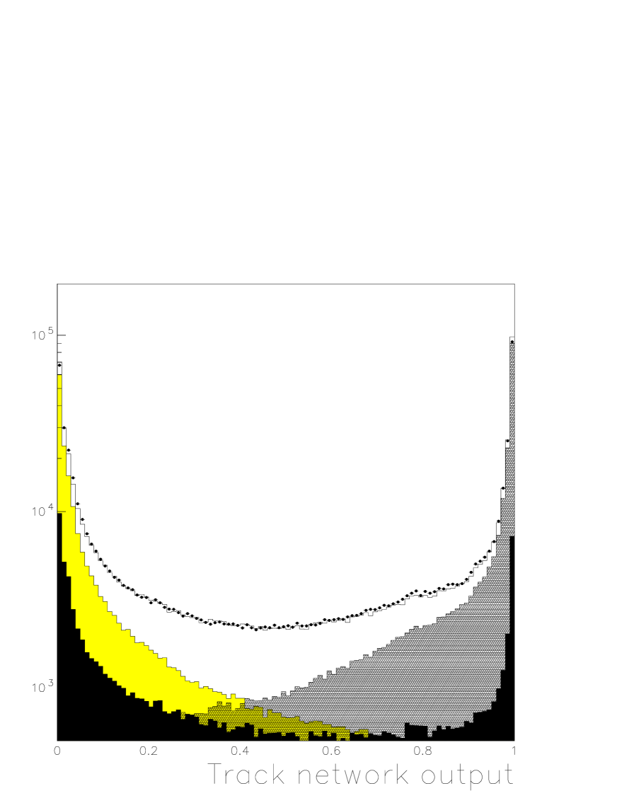
Distributions of all discriminating variables are shown in Figure 3.
 |
 |
 |
 |
 |
 |
 |
 |
 |
Two points should be noted. Firstly, to first approximation the track probabilities to originate from the primary or secondary vertex as calculated by the BSAURUS or the AABTAG packages, are calculations of the same quantity. There are differences however in the way track errors are handled in the two cases and, in addition, the AABTAG package returns a probability tuned to the resolution seen in the data. For these reasons, the correlation in these variables between the two methods is not 100% and there is extra information to be gained by including all definitions as input variables to the network. Secondly, the decay length variable (which is the same for all tracks in a given hemisphere) and the track quality word do not a priori distinquish between B-decay products and the background. These variables do however provide the network with information about whether the hemisphere has a well separated secondary vertex and whether the information associated with a particular track is reliable or not. This additional information has been found to be useful during the network training procedure.
The network therefore consists of 11 input nodes, one for each of the variables listed above, 12 nodes in the hidden layer, and a single output node with target value 1 for signal tracks and 0 for background. The training and performance samples are drawn only from Monte Carlo where signal tracks are defined as coming from any point along the weak B-decay chain, and background as coming from any source located at the primary vertex e.g. fragmentation and excited B-hadrons. The network training was performed using 30K signal and 30K background tracks in both the training and performance samples. The network output and performance for tagging tracks from B-decay are shown in Figures 4 and 5.

6 B-Species Identification(SHBN)
BSAURUS returns in the output variables, BSHEM(IBH_PRBBP,IH), BSHEM(IBH_PRBB0,IH),
BSHEM(IBH_PRBBS,IH) and BSHEM(IBH_PRBLB,IH) the probability for the
hemisphere IH to contain a or B-baryon respectively.
444The charge conjugate states are also implied.
The approach
employed is to supply all discriminating variables to a neural network
with four output nodes, one for each B-hadron type.
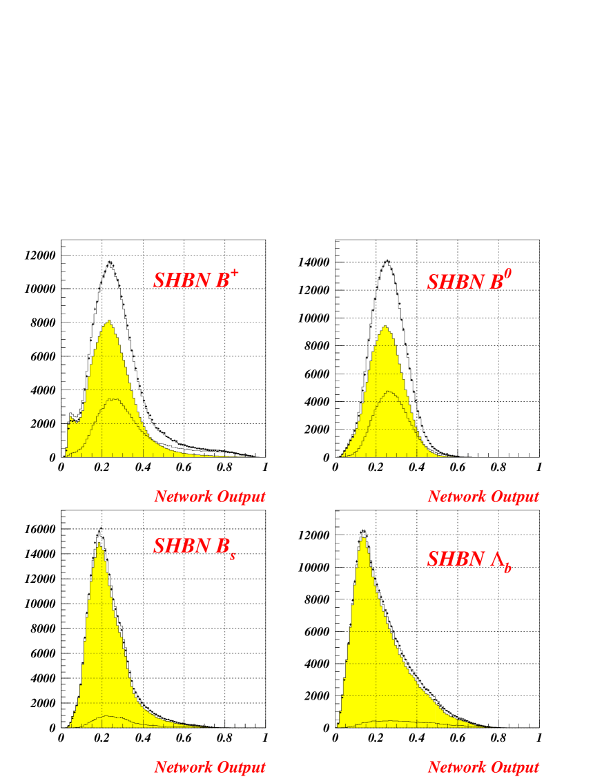
The resulting Same Hemisphere B-species enrichment Network or SHBN, consists of 15 input nodes(described below) and 17 nodes in the single hidden layer. Each output node delivers a probability for the hypotheses it is trained on i.e. the first supplies the probability for a meson to be produced in the hemisphere, the second for a meson, the third for charged mesons and the fourth for all species of B-baryons. The following input variables are used:
-
•
Using the TrackNet value as a probability () for each track to originate from the B-hadron decay vertex rather than from the primary vertex, the weighted vertex charge is formed
(4) that distinguishes between charged and neutral B-hadrons and is illustrated in Figure 6.
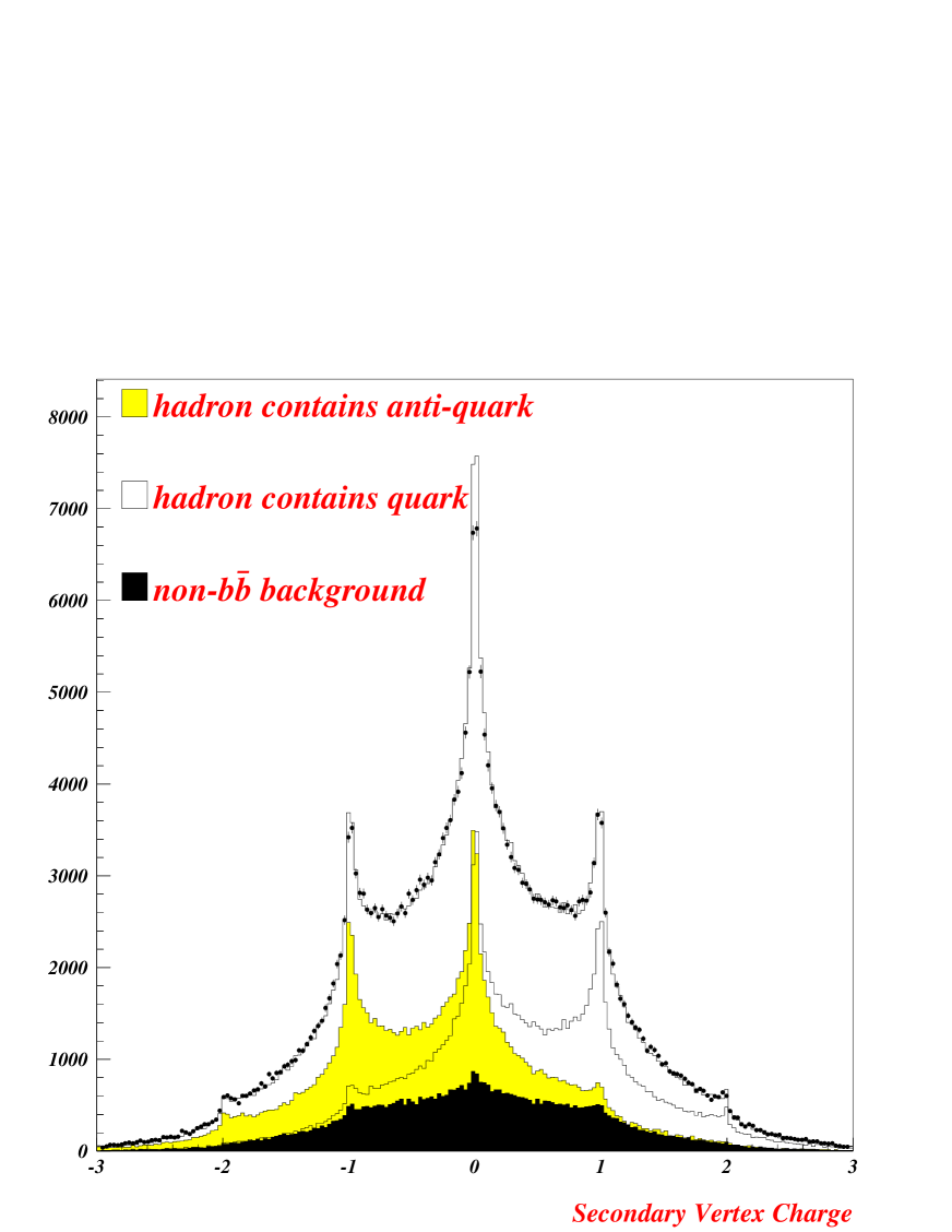
Figure 6: The vertex charge variable comparing data(points) to simulation(histogram) and showing separately the contributions from neutral, positively and negatively charged B-hadrons. Selection cuts and weights have been applied as detailed in Appendix A. -
•
The binomial error on the vertex charge, defined as
(5) gives a measure of the reliability of the vertex charge information.
-
•
The number of charged pions in the hemisphere. This is most powerful for the case of B-baryons and mesons, which have a higher content of non-pion particles, i.e. neutrons, protons and kaons in comparison to other B-species.
-
•
The total energy deposited in the hemisphere by charged and neutral particles scaled by the LEP beam energy. This is sensitive to the presence of B-baryons and mesons, due to the fact that associated neutrons and are often not reconstructed in the detector, with the consequence that the total hemisphere energy tends to be smaller compared to or mesons.
-
•
mesons are normally produced with a charged kaon as leading555The term leading refers to the neighbouring hadron to the B-hadron that emerges from the fragmentation chain. This particle is identified in practice from the fact that it often has the largest rapidity with respect to the B-hadron flight direction. fragmentation particle with a further kaon emerging from the weak decay (the same applies to the associated production of protons with B-baryons). Exploiting this fact, input variables are constructed giving the likelihood for the presence of a leading fragmentation kaon/proton and a kaon/proton weak decay product, for each of the two hypotheses; or B-baryon.
Utilising the Monte Carlo truth information, normalised track rapidity distributions were parameterised with Gaussians separately for the case of leading fragmentation tracks and B-decay products. These were then used to form a weight per reconstructed track which was summed over to give a hemisphere level variable. Cuts were applied for kaon or proton identification (see Section 2.6) and in order to separate the fragmentation tracks from the B-decay tracks via the TrackNet output.
-
•
The leading fragmentation track also can often be neutral e.g. production of a associated with meson production or associated with B-baryon production. An input was therefore constructed based on the presence of a reconstructed or in the hemisphere in the same way as for charged kaons and protons described above. In this case, the rapidity distribution was formed from Monte Carlo truth information for neutral particles originating from the primary vertex. The resulting weights were then summed over for reconstructed neutral particles with DELPHI mass codes 61 or 81 identifying and candidates.
-
•
The probability for the leading fragmentation particle to be a charged kaon. Specifically, the maximum kaon net output from the three tracks with highest rapidity originating from the primary vertex (via the condition TrackNet) was used. The three kaon probabilities can be found in BSAURUS outputs,
BSHEM(IBH_KRANK1,IH),BSHEM(IBH_KRANK2,IH),BSHEM(IBH_KRANK3,IH). -
•
A charge correlation between the leading fragmentation particle charges provided a flag for the presence of mesons. Specifically, the rapidity-weighted track charge sum over all tracks in the hemisphere is formed, and this is then scaled by the measured vertex charge.
In addition, input variables that gave no inherent separation power between different B species were included to inform the network of the potential quality of the other input variables:
-
•
the invariant mass of the reconstructed vertex,
-
•
the hemisphere quality factor described in Section 3.5,
-
•
the energy of the B-hadron, to provide information on how hard the fragmentation was and therefore inform the network of how the available energy is expected to be shared between B hadron and fragmentation products.
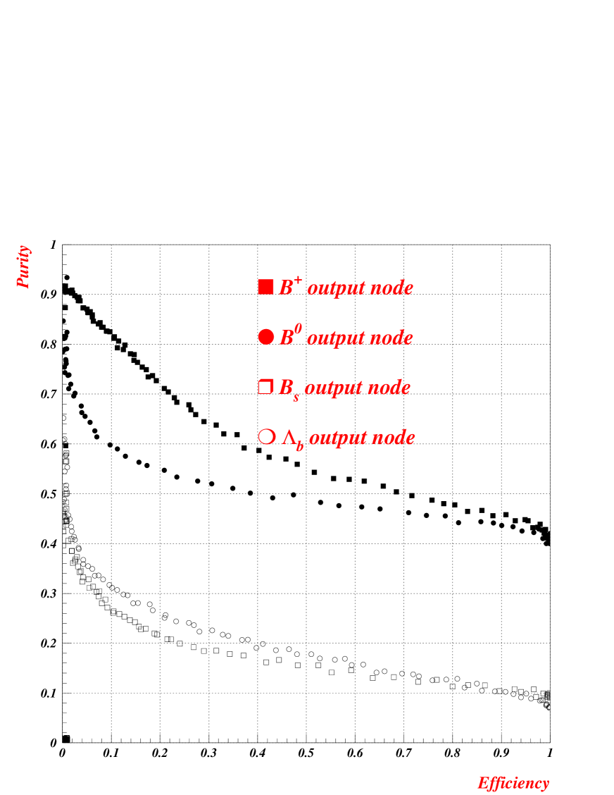
The output of the SHBN in both simulation and data is shown in Figure 7 and the resulting performance of the SHBN is shown in Figure 8.
The performance can be further improved by the combination of charge correlation information from the opposite hemisphere to form the Both Hemispheres B-species enrichment Network or BHBN. This network is described in Section 8.3.1.
7 B-D Separation(BDnet)
In selecting tracks for inclusion in the B-secondary vertex fit described in Section 3.1, there is inevitably some background from tracks that originate not from the B-decay vertex directly, but from the subsequent D-cascade decay point. The effect of including such tracks is illustrated in Figure 9 which shows that, on average, the B-decay length estimate reconstructed by BSAURUS lies somewhere between the true B decay point and that of the cascade D.
The BDnet is a neural network designed to discriminate between tracks originating from the weakly decaying B-hadron and those from the subsequent cascade D-meson decay. This information is clearly crucial to any algorithm wishing to eliminate the positive decay length bias just described, and is also used extensively throughout BSAURUS, particularly in the construction of B-flavour tags (e.g. see Section 8.1).
The following discriminating variables are used:
-
•
The angle between the track vector and an estimate of the B flight direction (taken to be
BSHEM(IBH_BTT,IH)). -
•
The probability that the track originates from the fitted primary vertex (AABTAG algorithm).
-
•
The probability that the track originates from the fitted secondary vertex (AABTAG algorithm).
-
•
The momentum and angle of the track vector in the B rest frame.
-
•
The TrackNet output.
-
•
The kaon network output, described in Section 2.6.
-
•
The lepton identification, see Section 2.6.
The remaining variables carry no implicit discriminating power but are included as gauges of the quality of the other variables:
-
•
The track quality word from Section 3.5.
-
•
The hemisphere quality word from Section 3.5.
-
•
The hemisphere decay length significance, .
-
•
The hemisphere secondary vertex mass.
-
•
The hemisphere rapidity gap between the track of highest rapidity below a TrackNet cut at 0.5 and that of smallest rapidity above the cut at 0.5.
The network architecture consisted of 14 input nodes with 15 nodes in a hidden layer and with a single output node trained on equal numbers of tracks directly from B-decay as ‘signal’ or from the following D-decay as ‘background’. Figure 10 shows the output of the network for the two classes of track used in training and Figure 11 plots the performance of the tag.


8 Optimal Fragmentation, Decay Flavour and Decay Type Tagging
In an attempt to use the information available optimally, the BSAURUS approach to tagging the flavour, i.e. charge of the b-quark, works by first constructing a probability per track and then combining these to give a probability at the hemisphere level.
Separate neural networks are trained to tag the underlying quark charge for the cases when there was a or B-baryon produced in the hemisphere. In addition two sets of such networks are produced, one trained only on tracks originating from the fragmentation process and the other trained only on tracks originating from weak B-hadron decay.
8.1 The Basis of Optimal Flavour Tagging
The basis of optimal flavour tagging is to construct, at the track level, the conditional probability for the track to have the same charge as the b-quark in the B-hadron both at the moment of fragmentation (i.e. production) and at the moment of decay. In addition, these probabilities are constructed separately for each of the B-hadron types; and B-baryon.
A neural network is used with a target output value of +1(-1) if the track charge is correlated(anticorrelated) with the b-quark charge. The discriminating input variables used are the following:
-
•
Particle identification variables (see Section 2.6):
-
–
kaon network output,
-
–
proton network output,
-
–
electron network output,
-
–
muon classification code.
-
–
-
•
B-D vertex separation variables:
-
–
BDnet output,
-
–
, where is the BDnet value, is the minimum BDnet value for all tracks in the hemisphere above a TrackNet value of 0.5, and is the difference between and ,
-
–
the momentum of the track in the B-candidate centre of mass frame.
-
–
-
•
Track-level quality variables:
-
–
the helicity angle of the track vector in the B-candidate centre of mass frame,
-
–
the track quality as defined in Section 3.5,
-
–
the TrackNet output,
-
–
the track energy.
-
–
-
•
Hemisphere-level quality variables:
-
–
the hemisphere rapidity gap between the track of highest rapidity below a TrackNet cut at 0.5 and that of smallest rapidity above the cut at 0.5,
-
–
the hemisphere quality as defined in Section 3.5,
-
–
the number of tracks in the hemisphere passing the standard cuts (Section 2.2) and with a TrackNet value greater than 0.5,
-
–
as defined above,
-
–
the secondary vertex mass,
-
–
the secondary vertex fit probability,
-
–
the ratio of the B-energy, defined by the
BSHEM(IBH_BTT,IH), to the LEP beam energy, -
–
the error on the vertex charge measurement.
-
–
In total, the track decay flavour network used all input variables described above in a network containing two hidden layers with 20 nodes in the first and 3 in the second. The track production flavour network used the same input variables without the lepton identification and B-D vertex separation variables, with 19 nodes in the first hidden layer and 3 in the second.


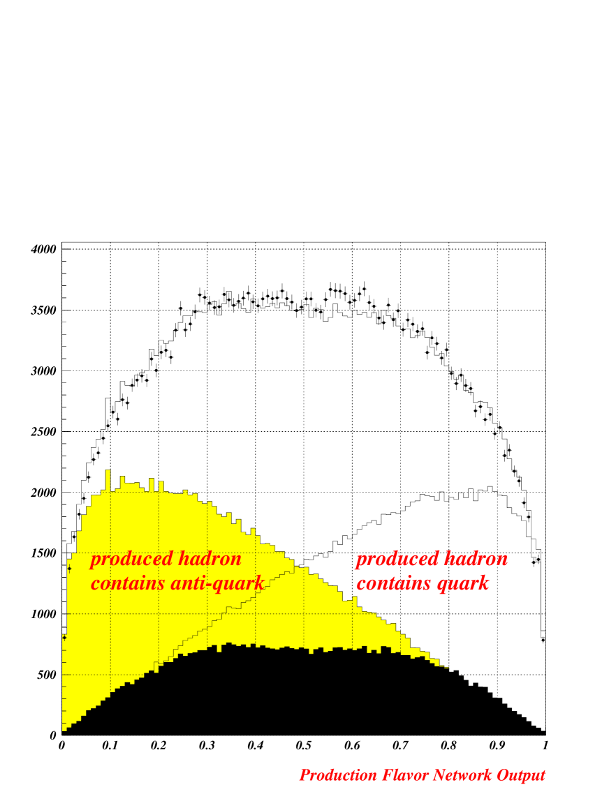
The resulting track charge correlation conditional probabilities
are plotted in Figure 12 for the case of fragmentation
flavour and in Figure 13 for the case of decay flavour.
Figures 14 and 15 show the
corresponding tag performance attained by the
fragmentation and decay flavour probabilities respectively.
These outputs can be found in BSAURUS variables;
BSPAR(IBP_FFLBS,IT),BSPAR(IBP_FFLB0,IT),
BSPAR(IBP_FFLBP,IT) and BSPAR(IBP_FFLLB,IT)
for the fragmentation flavour conditional probabilities and in
BSPAR(IBP_DFLBS,IT),BSPAR(IBP_DFLB0,IT),
BSPAR(IBP_DFLBP,IT) and BSPAR(IBP_DFLLB,IT)
for the decay flavour conditional probabilities.


Finally, to obtain a flavour tag at the hemisphere level, the conditional track probabilities described above, where or B-baryon and or , are combined as the likelihood ratio,
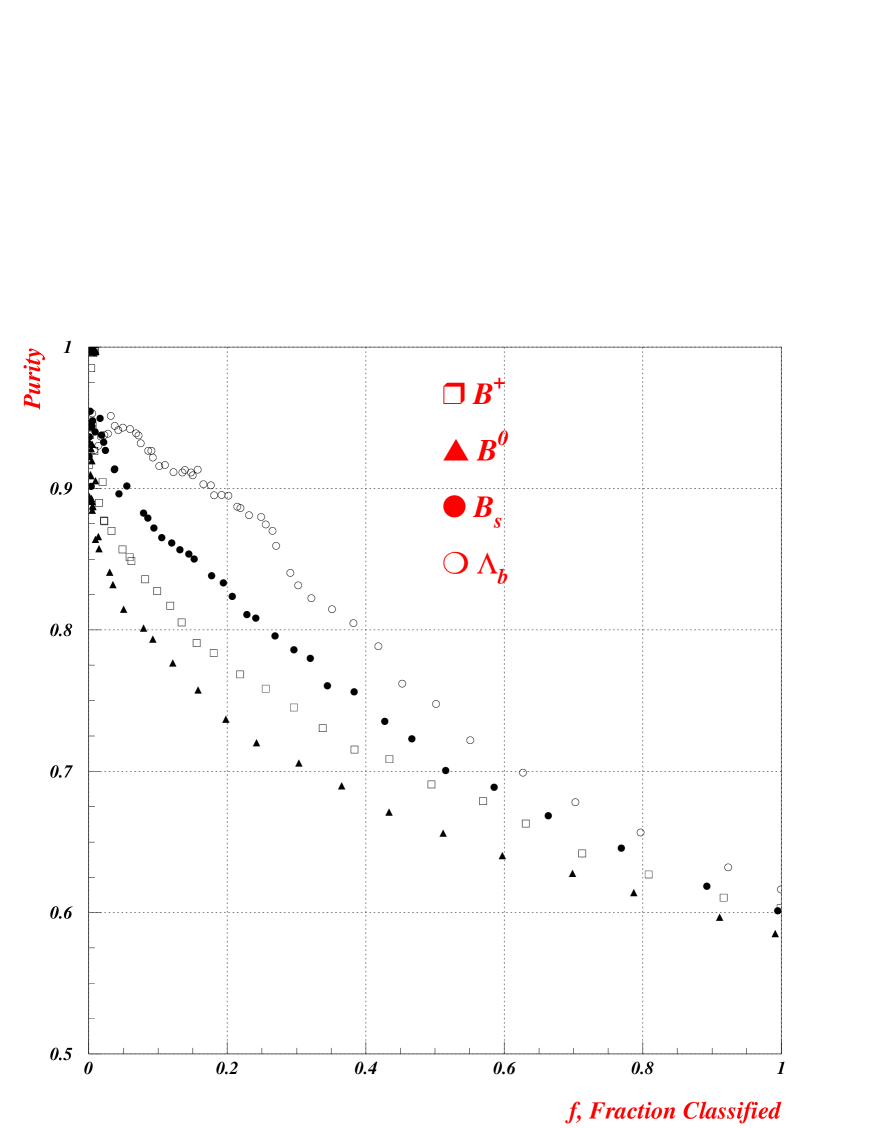
where is the track charge. Which tracks to sum over depends on the hypothesis considered, i.e. for the fragmentation flavour it is over all tracks with TrackNet whilst for the decay flavour, tracks must satisfy TrackNet. These hemisphere flavour tags are compared with the data in Figure 16 for the fragmentation tag, and in Figure 17 for the decay tag.
The purity against efficiency performance of the tags are
shown in Figure 18 for the fragmentation tag
and in Figure 19 for the decay tag.
The tags are located in the following BSAURUS variables;
BSHEM(IBH_FFLBS,IH), BSHEM(IBH_FFLB0,IH),
BSHEM(IBH_FFLBP,IH) and BSHEM(IBH_FFLLB,IH)
for the production flavour outputs and in
BSHEM(IBH_DFLBS,IH), BSHEM(IBH_DFLB0,IH),
BSHEM(IBH_DFLBP,IH) and BSHEM{IBH_DFLLB,IH)
for the decay flavour outputs.

8.2 Applications to Production Flavour Tagging
8.2.1 The Same Hemisphere Production flavour Network (SHPN)
The hemisphere flavour tags described in Section 8.1 form the major input to a further dedicated network, the Same Hemisphere Production flavour Network or SHPN. This network attempts to find the optimal combination of fragmentation and decay flavour, for each B-species hypothesis, in order to tag the B-hadron quark flavour at production time. The network is constructed independently of any information from the opposite hemisphere, primarily so that the output can be used for a measurement[10] incorporating double-hemisphere flavour tag methods.
The 9 input variables used are (ignoring some details of variable transformation and re-scaling):
-
•
-
•
-
•
-
•
, where is the reconstructed B-lifetime. Note this construction takes account of the oscillation frequency found in the simulation. This is not possible for the case of where the oscillations are so fast that we have essentially a 50-50 mix of and .
-
•
The jet charge defined as,
(6) where the sum is over all tracks and is the longitudinal momentum component to the thrust axis. The optimal choice of the free parameter depends on the type of B-hadron under consideration. For this application we choose a range of values where the last value corresponds to taking the charge of the stiffest track in the hemisphere.
- •
-
•
Vertex charge significance.
Note that the factors represent the outputs of the B-species tagging network, SHBN, described in Section 6.
The treatment of quality variables is slightly different for this network compared to other BSAURUS networks. In this case, in order to ensure that the output is inherently symmetric with respect to opposite charges, the quality variables are used to weight the turn-on gradient (or ‘temperature’) of the sigmoid function used as the network node transfer function. This restriction is especially important for analyses such as measurements of which to first order implicitly assume that the charge tag used is symmetric with respect to quark and anti-quark. The quality variables used were:
-
•
The hemisphere quality word
BSHEM(IBH_QUAL2,IH)described in Section 3.5. -
•
The hemisphere rapidity gap between the track of highest rapidity below a TrackNet cut at 0.5 and that of smallest rapidity above the cut at 0.5.
-
•
The error on the vertex charge measurement.
-
•
The ratio of the B-energy, defined by the
BSHEM(IBH_BTT,IH), to the LEP beam energy.
The SHPN output is stored in BSAURUS variable
BSHEM(ISH_FLAV45,IH)
and is compared to the data in
Figure 20.
The performance of the tag can be seen in Figure 21(full circles).

8.2.2 The Both Hemispheres Production flavour Network (BHPN)
It should be noted that an improved performance for production flavour tagging can be obtained by including the information from the opposite side hemisphere. The Both Hemispheres Production flavour Network or BHPN is defined as the ratio,
| (7) |
where the labels and refer to the production tag
in this hemisphere and in the opposite hemisphere respectively.
Note that if SHPN tags e.g. the charge of the quark, then
tags the charge of the anti-quark.
The resulting performance of the BHPN is also shown in
Figure 21(open circles) and the output
can be found in BSAURUS output BSHEM(IBH_FLBOTH,IH).
8.3 Applications to Decay Type and Decay Flavour Tagging
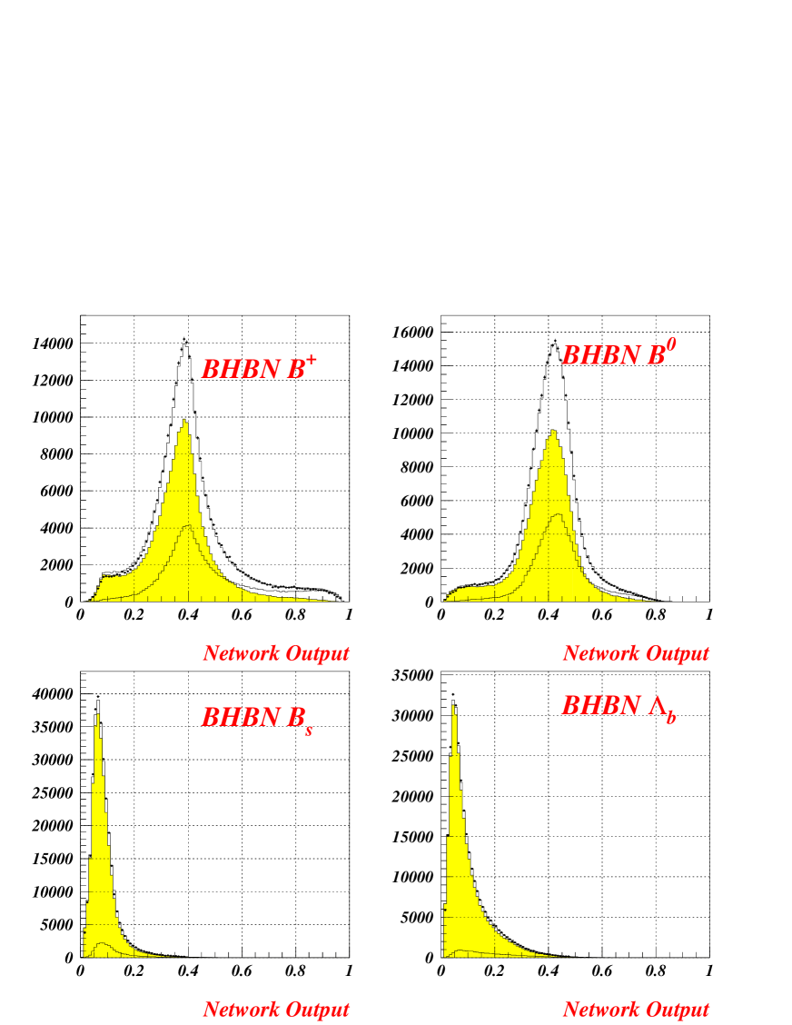
8.3.1 Both Hemispheres B-species enrichment Network (BHBN)
The performance of the SHBN (Section 6) can be further improved by use of the hemisphere flavour tags developed in Section 8 and by the introduction of charge correlation information from the opposite hemisphere to form the Both Hemispheres B-species enrichment Network or BHBN.
In the same way as for the SHBN, the BHBN is a network with four output target nodes, one for each B-type, 16 input nodes and two hidden layers consisting of 20 and 10 nodes respectively. The input variables used, ignoring some details of variable scaling and transformation, are as follows: We define the variable, , which is proportional to the production flavour tag SHPN(see Section 8.2) in the opposite hemisphere, but scaled by a function in in an attempt to explicitly account for the b-quark forward-backward asymmetry,
The discriminating variables used are:
-
•
SHBN probability for , .
-
•
SHBN probability for , .
-
•
SHBN probability for , .
-
•
SHBN probability for B-baryon, .
-
•
-
•
-
•
-
•
-
•
-
•
-
•
-
•
-
•
Where the terms are the hemisphere flavour likelihood ratios described in Section 8.1. The quality variables used are:
-
•
The hemisphere quality word
BSHEM(IBH_QUAL2,IH)described in Section 3.5. -
•
The hemisphere rapidity gap between the track of highest rapidity below a TrackNet cut at 0.5 and that of smallest rapidity above the cut at 0.5.
-
•
The ratio of the B-energy, defined by the
BSHEM(IBH_BTT,IH), to the LEP beam energy.
The outputs of the BHBN are plotted in Figure 22 and can be found
in BSAURUS variables,
BSHEM(IBH_PRBAIBP,IH), BSHEM(IBH_PRBAIB0,IH),
BSHEM(IBH_PRBAIBS,IH) and BSHEM(IBH_PRBAILB,IH).
The resulting performance of the network is shown in figure 23.

8.3.2 The Both Hemispheres Decay Flavour Network(BHDN)
The Both Hemispheres Decay flavour Network or BHDN, utilises similar constructions for the discriminating variables as in the SHPN, the main difference being that opposite side hemisphere information is explicitly used in order to boost the performance.
We define the variable, , which is proportional to the production flavour tag in the opposite hemisphere, , but scaled by a function in in an attempt to explicitly account for the b-quark forward-backward asymmetry,
| (8) |
The discriminating variables used are:
-
•
-
•
-
•
-
•
, where is the reconstructed B-lifetime.
Note that the factors represent the outputs of the B-species tagging network, BHBN which includes information from the opposite side hemisphere, and is described in Section 6. The quality variables used were:
The output of the decay flavour net is stored in BSAURUS word
BSHEM(ISH_DFLAV45,IH)
and the performance of the tag is also shown in
Figure 21(open squares).
BSAURUS routine, DECFLA, gives the user the option to
recalculate the decay flavour network output based only on
a list of tracks that he/she supplies. This can be useful in analyses
that need to avoid potential biases in the flavour tag.
Summary and Outlook
The BSAURUS package reconstructs properties of B-hadron decays inside the jets of events in an intrinsically inclusive way in order to ensure high efficiency. Exploiting wherever possible, physics knowledge of b-quark production, the hadronisation process and of the subsequent B decay, this information is combined to tag quantities of importance for B-physics analyses. In order to combine information in an optimal way, i.e. to ensure high purity, neural network techniques are used extensively.
This note has described how this approach is applied to DELPHI data in order to form, most importantly, variables that tag the presence of a or B-baryon and variables that tag the charge or flavour of the b-quark in any of the B-hadron types at production and decay time separately. These tags are fundamental inputs to B-physics analyses such as B-spectroscopy[7], B-species lifetime measurements[8], and oscillations[9], the forward-backward asymmetry in events[10], the measurement of B-hadron production fractions[11] and measurements of B-hadron branching ratios[12]. Analyses in all these areas have either already been completed or are currently underway in DELPHI using the BSAURUS framework. In addition, the list is by no means exhaustive and new analyses are currently being planned e.g. measuring the fragmentation function of B-species and studies of radially excited B-meson states.
It should be noted that the package is under constant and on-going
development. New features and improvements are still being added
and this is likely to continue in the future. All news and new
features relating to BSAURUS are documented at the web-site
location:
http://pubxx.home.cern.ch/pubxx/tasks/bcteam/www/inclusive/bsaurus.html.
Acknowlegements
The authors would like to acknowlege the contributions of Oliver Podobrin and Christof Kreuter, who were instrumental in developing the origional version of BSAURUS. In addition, Christian Weiser has made some valuable contributions. We would also like to thank Wilbur Venus for his detailed reading of the manuscript.
Appendix A: Cuts and Weights Applied to BSAURUS performance Plots
Where indicated, the following cuts have been applied to the event sample entering the distribution shown:
-
•
BSAURUS word,
ISAURUS(IH), for hemisphere numberIHmust have value 4 or higher indicating that the secondary vertex fit in this hemisphere converged normally. -
•
Combined event b-tag.
-
•
2-jet events only.
-
•
.
In addition, to account for known differences between
data and Monte Carlo arising from both detector effects
and physics modelling, the simulation has been
weighted (via BSAURUS routine SIMWAIT,
stored in output BSHEM(IBH_WEIGHT,IH)) to
account for:
-
•
The differences between data and Monte Carlo in the hemisphere quality variable
BSHEM(IBH_QUAL,IH)as a function of the hemisphere track multiplicity,BSHEM(IBH_NPGOOD,IH). -
•
Latest world average B-species production fractions.
-
•
Latest world average B-species lifetime measurements.
-
•
MARKIII D-topological branching fractions.
-
•
Any remaining difference between data and Monte Carlo in the B-energy estimate i.e. variable
BSHEM(IBH_BTT+3,IH).
Note that the current measurements of B-physics quantities used to form weights, are chosen to follow LEP Working Group recommendations.
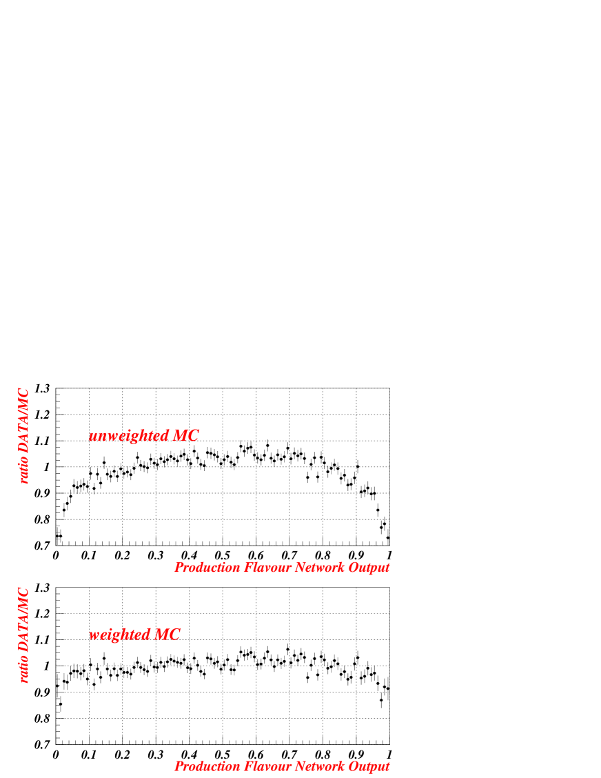
Figure 24 shows the effect, for example,
on the production
flavour network output of applying the weight returned by
routine SIMWAIT. The much improved agreement between
data and simulation after the weight is applied illustrates
the need for such a correction if the network outputs are
used in analyses to estimate e.g. absolute efficiencies.
Appendix B: How to Access BSAURUS Outputs
A call to routine BSAURUS should be made once per
event from the user routine. A list of the BSAURUS outputs
at track, hemisphere and event level is given in Appendix C.
BSAURUS uses a modified version of the VECSUB package, called
VECTOP, to fill the standard track information array
P(NDIM,*).
Of the utmost importance to users running the standard VECSUB
package e.g. SKELANA users, is the track output
word, BSPAR(IBP_IYB,IT).
This gives the matching VECSUB track index for BSAURUS
(ie VECTOP) track IT. Users failing to do this track matching
will certainly obtain the wrong results from BSAURUS.
The BSAURUS-cards file is released periodically to the
standard DELPHI areas for library creation. A development
version is to be found at:
/afs/cern.ch/user/b/barker/public/delphi/bsaurus.car.
Naturally, the results of using this version cannot
be guaranteed.
Appendix C: BSAURUS output array definitions
Quantities calculated in BSAURUS along with other variables, e.g. truth Monte Carlo information, that are useful for analyses are available via COMMON /CSAURUS/ at the event, hemisphere and track level.
1) The event output array:
*     Array Element     Number of           Description
*                        values
*    -----------------------------------------------------------------
*     BSEVT(IBE_BTAG)      1     event B-tag
*     BSEVT(IBE_BCONF)     1     event B-confidence (Bill Murray)
*     BSEVT(IBE_BCTAG)     1     event B-tag with charm suppression
*     BSEVT(IBE_BCOMB)     1     event aabtag combined-tag
*     BSEVT(IBE_PV)        3     primary vertex
*     BSEVT(IBE_PC)        6     primary covariance matrix
*     BSEVT(IBE_NJET)      1     number of jets
*     BSEVT(IBE_COST)      1     COS(theta) of event thrust axis
*     BSEVT(IBE_RICH)      1     Barrel RICH status: 3=gas+liq.,2=liq. only
*                                ,1=gas only, 0=no liq. or gas
*     BSEVT(IBEMC_FLAV)    1     MC primary quark flavour (e.g. 12=b)
*     BSEVT(IBEMC_PV)      3     MC primary vertex
2) The hemisphere output array where IHEM is the hemisphere number (1 or 2):
*     Array Element     Number of           Description
*                        values
*     -----------------------------------------------------------------
*     BSHEM(IBH_HNUM,IHEM)     1   hemisphere number
*     BSHEM(IBH_BTAG,IHEM)     1   hemisphere B-tag
*     BSHEM(IBH_BCONF,IHEM)    1   hemisphere B-confidence (Bill Murray)
*     BSHEM(IBH_BCTAG,IHEM)    1   hemisphere B-tag with charm suppression
*     BSHEM(IBH_BCOMB,IHEM)    1   hemisphere aabtag combined tag
*     BSHEM(IBH_BJET,IHEM)     4   hemisphere B-candidate jet 4-vector
*     BSHEM(IBH_NJET,IHEM)     1   number jets in hemisphere

*     BSHEM(IBH_BF,IHEM)       4   B 4-vector from fit
*     BSHEM(IBH_BT,IHEM)       4   B 4-vector from fit + energy correction
*     BSHEM(IBH_BY,IHEM)       4   B RAW 4-vector: from rapidity algorithm
*                                for 3-jet, net weighted for 2-jet
*     BSHEM(IBH_BTT,IHEM)      4   ’optimal’ B 4-vector
*     BSHEM(IBH_SV,IHEM)       3   secondary vertex coordinates
*     BSHEM(IBH_SC,IHEM)       6   secondary vertex covariance matrix
*     BSHEM(IBH_SIGPHI,IHEM)   1   Error on direction phi from SV fit
*     BSHEM(IBH_SIGTHET,IHEM)  1   Error on direction theta from SV fit
*     BSHEM(IBH_DEC,IHEM)      1   B decay length
*     BSHEM(IBH_DECS,IHEM)     1   B decay length error
*     BSHEM(IBH_PROB,IHEM)     1   secondary vertex fit probability
*     BSHEM(IBH_RET,IHEM)      1   ISAURUS - fit return code
*     BSHEM(IBH_YBFIT,IHEM)    1   YBFIT2  - secondary vertex fit return code
*     BSHEM(IBH_NACC,IHEM)     1   no. of particles at sec. vertex
*     BSHEM(IBH_QJET,IHEM)     1   jet charge, kappa=0.6
*     BSHEM(IBH_QJET2,IHEM)    1   jet charge, kappa=0.3
*     BSHEM(IBH_QJET3,IHEM)    1   jet charge, stiffest track in P_L
*     BSHEM(IBH_QVER,IHEM)     1   Vertex charge NN
*     BSHEM(IBH_QVERS,IHEM)    1   Vertex charge NN error
*     BSHEM(IBH_RAWQ,IHEM)     1   Vertex charge (sum trk. charge)
*     BSHEM(IBH_FLAV,IHEM)     1   Original b flavour NN
*     BSHEM(IBH_FLAV45,IHEM)   1   improved b flavour NN (<0.5->b, >0.5->bbar)
*     BSHEM(IBH_FLBOTH,IHEM)   1   likelihood combination with opp. side info.
*     BSHEM(IBH_MY,IHEM)       1   rapidity mass
*     BSHEM(IBH_SHEM,IHEM)     1   scaled measured hemisphere energy
*     BSHEM(IBH_SHEM2,IHEM)    1   scaled measured hemisphere energy (2-BODY)
*     BSHEM(IBH_QUAL,IHEM)     1   hemisphere quality flag:
*                                  N(rejected trk cuts)+100*N(interactions)+
*                                  1,000N(ambiguous hits)+100,000*N(ISRT=0)
*     BSHEM(IBH_QUAL2,IHEM)    1   Continous hemisphere quality 0-(perfect)10(bad)
*     BSHEM(IBH_MVER,IHEM)     1   Mass on secondary vertex
*     BSHEM(IBH_BPLUS,IHEM)    1   B+ tagging
*     BSHEM(IBH_BZERO,IHEM)    1   B0 tagging
*     BSHEM(IBH_PRPF,IHEM)     1   prim. vertex fragmentation Borisov prob
*     BSHEM(IBH_PRPB,IHEM)     1   prim. vertex B Borisov prob
*     BSHEM(IBH_PRSF,IHEM)     1   sec.  vertex fragmentation Borisov prob
*     BSHEM(IBH_PRSB,IHEM)     1   sec.  vertex B Borisov prob
*     BSHEM(IBH_DIPOL,IHEM)    1   sec.  vertex dipole moment
*     BSHEM(IBH_HKST,IHEM)     1   Q*PMIN of tracks in B CMS
*
*     BSHEM(IBH_NPALL,IHEM)    1   # of particles
*     BSHEM(IBH_NPGOOD,IHEM)   1   # of particles past quality cuts
*     BSHEM(IBH_NPCUT,IHEM)    1   # particles past IBP_NET > PNET_CUT
*     BSHEM(IBH_NPGC,IHEM)     1   # past IBP_NET>PNET_CUT + qual. requirement
*     BSHEM(IBH_NKS,IHEM)      1   # recon. K_s with y>1.6
*     BSHEM(IBH_NWKSD,IHEM)    1   sum of y-prob. funct for decay K_s
*     BSHEM(IBH_NWKSF,IHEM)    1   sum of y-prob. funct for frag. K_s
*     BSHEM(IBH_NLAM0,IHEM)    1   # recon. Lambda(uds) with y>1.6
*     BSHEM(IBH_NWLAMBD,IHEM)  1   sum of y-prob. funct for decay lambdas
*     BSHEM(IBH_NWLAMBF,IHEM)  1   sum of y-prob. functions for frag.lambdas
*     BSHEM(IBH_NNEUT,IHEM)    1   # recon. neutrons with y>1.6
*     BSHEM(IBH_NPION,IHEM)    1   # charged pions
*     BSHEM(IBH_PICHRG,IHEM)   1   # pions charged weighted about SV
*     BSHEM(IBH_NKDECAY,IHEM)  1   Sum of  kaon weights for trknet> 0.5
*     BSHEM(IBH_NKFRAG,IHEM)   1   Sum of  kaon weights for < 0.5
*     BSHEM(IBH_NWKD,IHEM)     1   sum of y-prob. funct for decay K+/-
*     BSHEM(IBH_NWKF,IHEM)     1   sum of y-prob. functions for frag. K+/-
*     BSHEM(IBH_NPDECAY,IHEM)  1   Sum of proton weights for trknet > 0.5
*     BSHEM(IBH_NPFRAG,IHEM)   1   Sum of proton weights for trknet < 0.5
*     BSHEM(IBH_NWPROTD,IHEM)  1   sum of y-prob. functions for decay protons
*     BSHEM(IBH_NWPROTF,IHEM)  1   sum of y-prob. functions for frag. protons
*     BSHEM(IBH_QKAMAX,IHEM)   1   MAX. q*trknet in hemisphere for tight K.
*     BSHEM(IBH_PKAON,IHEM)    1   charge correl. coeff. best kaon cand. in hem
*     BSHEM(IBH_QKAON,IHEM)    1   charge of best kaon cand. in hemisphere
*     BSHEM(IBH_PLEP,IHEM)     1   charge correlation coeff. of best lep
*     BSHEM(IBH_QLEP,IHEM)     1   charge of best lepton cand. in hemisphere
*
*     BSHEM(IBH_DEC3D,IHEM)    1   3 D decay length
*     BSHEM(IBH_DEC3DS,IHEM)   1   error on 3 D decay length
*     BSHEM(IBH_BLIFE,IHEM)    1   B lifetime
*     BSHEM(IBH_BLIFES,IHEM)   1   error on B lifetime
*     BSHEM(IBH_CHRDIP,IHEM)   1   B-D charge dipole moment from GBDIPOLE
*     BSHEM(IBH_SVVAR1,IHEM)   1   Mean deviation of trks about SV point
*     BSHEM(IBH_SVVAR2,IHEM)   1   Mean square deviation
*     BSHEM(IBH_DIPPY,IHEM)    1   A dipole moment from the SVVAR-calc
*
*     BSHEM(IBH_QRANK1,IHEM)   1   Charge of leading frag. track
*     BSHEM(IBH_QRANK2,IHEM)   1   Charge of 2ND rank frag track
*     BSHEM(IBH_QRANK3,IHEM)   1   Charge of 3RD rank frag track
*     BSHEM(IBH_YRANK1,IHEM)   1   Rapidity of leading frag track
*     BSHEM(IBH_YRANK2,IHEM)   1   Rapidity of 2ND rank frag track
*     BSHEM(IBH_YRANK3,IHEM)   1   Rapidity of 3RD rank frag track
*     BSHEM(IBH_KRANK1,IHEM)   1   Kaon net for leading rank frag track
*     BSHEM(IBH_KRANK2,IHEM)   1   Kaon net for 2ND rank frag track
*     BSHEM(IBH_KRANK3,IHEM)   1   Kaon net for 3RD rank frag track
*     BSHEM(IBH_PRANK1,IHEM)   1   Proton net for leading rank frag track
*     BSHEM(IBH_PRANK2,IHEM)   1   Proton net for 2ND rank frag track
*     BSHEM(IBH_PRANK3,IHEM)   1   Proton net for 3RD rank frag track
*     BSHEM(IBH_DELTA,IHEM)    1   delta - y-gap above/below trknet=0.5
*     BSHEM(IBH_QFSUM,IHEM)    1   Sum of frag. track charge
*     BSHEM(IBH_DFLBS,IHEM)   1   decay flavour net for B_s
*     BSHEM(IBH_DFLB0,IHEM)   1   decay flavour net for B0
*     BSHEM(IBH_DFLBP,IHEM)   1   decay flavour net for B+
*     BSHEM(IBH_DFLLB,IHEM)   1   decay flavour net for LamB
*     BSHEM(IBH_FFLBS,IHEM)   1   fragmentation flavour net for B_s
*     BSHEM(IBH_FFLB0,IHEM)   1   fragmentation flavour net for B0
*     BSHEM(IBH_FFLBP,IHEM)   1   fragmentation flavour net for B+
*     BSHEM(IBH_FFLLB,IHEM)   1   fragmentation flavour net for LamB
*     BSHEM(IBH_PRBBS,IHEM)   1   probability for B_s  from all-flavour net
*     BSHEM(IBH_PRBB0,IHEM)   1   probability for B0   from all-flavour net
*     BSHEM(IBH_PRBBP,IHEM)   1   probability for B+   from all-flavour net
*     BSHEM(IBH_PRBLB,IHEM)   1   probability for LamB from all-flavour net
*     BSHEM(IBH_PRBAIBS,IHEM) 1   B_s  prob. from all-flavour net inc. opp. hem. info.
*     BSHEM(IBH_PRBAIB0,IHEM) 1   B0   prob. from all-flavour net inc. opp. hem. info.
*     BSHEM(IBH_PRBAIBP,IHEM) 1   B+   prob. from all-flavour net inc. opp. hem. info.
*     BSHEM(IBH_PRBAILB,IHEM) 1   LamB prob. from all-flavour net inc. opp. hem. info.
*     BSHEM(IBH_DFLAV45,IHEM) 1   Optimal decay flavour net
*     BSHEM(IBH_LIKBS,IHEM)   1   Likelihood ratio prod. flav. tag for B_s
*     BSHEM(IBH_LIKB0,IHEM)   1   Likelihood ratio prod. flav. tag for B_d
*
*     BSHEM(IBH_WEIGHT,IHEM)  1   SIMWAIT weight for physics/quality differences
*                                 between simulation and data
*
*     BSHEM(IBHMC_BDEC2D,IHEM) 1   MC generated 2-d B decay length
*     BSHEM(IBHMC_BDEC,IHEM)   1   MC generated 3-d B decay length
*     BSHEM(IBHMC_DDEC,IHEM)   1   MC generated 3-d Dbar decay length
*     BSHEM(IBHMC_DPDEC,IHEM)  1   MC generated 3-d D decay length
*     BSHEM(IBHMC_BV,IHEM)     3   MC generated B vertex
*     BSHEM(IBHMC_DV,IHEM)     3   MC generated Dbar vertex
*     BSHEM(IBHMC_DPV,IHEM)    3   MC generated D vertex
*     BSHEM(IBHMC_DST,IHEM)    1   MC D* in hemisphere
*     BSHEM(IBHMC_BP,IHEM)     4   MC B 4-VECTOR
*     BSHEM(IBHMC_BKF,IHEM)    1   MC kf code for weakly decaying B
*     BSHEM(IBHMC_ND,IHEM)     1   MC: # of weakly decaying D
*     BSHEM(IBHMC_OSCB,IHEM)   1   MC flag for oscillating B*
*     BSHEM(IBHMC_BLIFE,IHEM)  1   MC B lifetime
*     BSHEM(IBHMC_BMC,IHEM)1   1   MC B charged decay multiplicity
*     BSHEM(IBHMC_BMTOT,IHEM)  1   MC B charged+neutral decay multiplicity
*     BSHEM(IBHMC_QTYP,IHEM)   1   MC produced quark flavour
*     BSHEM(IBHMC_PBKF,IHEM)   1   MC kf code for primary B
*     BSHEM(IBHMC_DRSKF,IHEM)  1   MC kf code for right sign D
*     BSHEM(IBHMC_QCDRS,IHEM)  1   MC charged decay mult. of right sign D
*     BSHEM(IBHMC_QNDRS,IHEM)  1   MC charged+neutral decay mult. of RSD
*     BSHEM(IBHMC_DRSP,IH)     1   MC P of the right sign D in the B CMS
*     BSHEM(IBHMC_SLD,IH)      1   MC 1=weak B has decayed to e or mu, 0=not
3) The track output array where IPART is the track number:
*     Array Element     Number of           Description
*                        values
*     -----------------------------------------------------------------
*     BSPAR(IBP_HEM,IPART)   1   hemisphere (or jet) number
*     BSPAR(IBP_IYB,IPART)   1   index of the matching VECSUB track
*     BSPAR(IBP_QUAL,IPART)  1   track quality: 20(if isrt=0) + 10(if from
*                                interaction) + 1(if has ambiguous hits)
*     BSPAR(IBP_Y,IPART)     1   rapidity with respect to jet
*     BSPAR(IBP_PRP,IPART)   1   probability to fit primary vertex
*     BSPAR(IBP_PRS,IPART)   1   probability to fit secondary vertex
*     BSPAR(IBP_BRP,IPART)   1   Borisov probability in rphi
*     BSPAR(IBP_BZ,IPART)    1   Borisov probability in z
*     BSPAR(IBP_B3D,IPART)   1   Borisov probability in 3D
*     BSPAR(IBP_BSRP,IPART)  1   Borisov probability in rphi w/r secondary vtx
*     BSPAR(IBP_BSZ,IPART)   1   Borisov probability in z  w/r secodary vtx
*     BSPAR(IBP_BS3D,IPART)  1   Borisov probability in 3D w/r secodary vtx
*     BSPAR(IBP_NET,IPART)   1   net output (-->0 for good fragmentation,
*                                            -->1 for good B decay product)
*     BSPAR(IBP_DNET,IPART)  1   cascade D track net output
*     BSPAR(IBP_NRP,IPART)   1   number of rphi VD hits
*     BSPAR(IBP_NZ,IPART)    1   number of z VD hits
*     BSPAR(IBP_KST,IPART)   1   momentum of track in B CMS
*     BSPAR(IBP_THETST,IPART)1   helicity angle of the track
*     BSPAR(IBP_BSAU,IPART)  1   pointer to BSAURUS internal particle array
*     BSPAR(IBP_SV,IPART)    1   1--> trk in sec. vertex 0--> trk not in SV
*     BSPAR(IBP_TRKE,IPART)  1   Track energy
*     BSPAR(IBP_TRKM,IPART)  1   Track mass
*     BSPAR(IBP_TRKP,IPART)  1   Track momentum
*     BSPAR(IBP_TRKQ,IPART)  1   Track charge
*     BSPAR(IBP_TRKL,IPART)  1   Track length
*     BSPAR(IBP_ERRE,IPART)  1   Error on track energy
*     BSPAR(IBP_DELPP,IPART) 1   Delta(P)/P
*     BSPAR(IBP_DFLBS,IPART) 1   charge/decay flavour correlation net for B_s
*     BSPAR(IBP_DFLB0,IPART) 1   charge/decay flavour correlation net for B0
*     BSPAR(IBP_DFLBP,IPART) 1   charge/decay flavour correlation net for B+
*     BSPAR(IBP_DFLLB,IPART) 1   charge/decay flavour correlation net for LamB
*     BSPAR(IBP_FFLBS,IPART) 1   charge/fragm. flavour correlation net for B_s
*     BSPAR(IBP_FFLB0,IPART) 1   charge/fragm. flavour correlation net for B0
*     BSPAR(IBP_FFLBP,IPART) 1   charge/fragm. flavour correlation net for B+
*     BSPAR(IBP_FFLLB,IPART) 1   charge/fragm. flavour correlation net for LamB
*     BSPAR(IBP_MACK,IPART)  1   MACRIB kaon net output
*     BSPAR(IBP_MACP,IPART)  1   MACRIB proton net output
*
*     BSPAR(IBPMC_KF,IPART)  1   MC Lund KF code
*     BSPAR(IBPMC_KFP,IPART) 1   MC Lund KF parent code
*     BSPAR(IBPMC_TYP,IPART) 1   MC code
*                                0 : unidentified
*                                1 : ordinary fragmentation
*                                2 : fragmentation partner of B-hadron
*                                3 : decay of primary (not weak) C
*                                4 : decay of D*
*                                5 : decay of weak B
*                                6 : decay of excited B
*                                7 : decay of weak C
*                                1x : same as for x but decay of
*                                     long living particles (e.g. K_l)
*                                2x : same as for x but from
*                                     hadronic interaction or photo conv.
*                                -/+ : b/bbar quark
*                                      6       : content of primary B
*                                      3,4,5,7 : content of weak B
*
*     BSPAR(IBPMC_KST,IPART)     1 MC momentum of track in MC B CMS
*     BSPAR(IBPMC_THETST,IPART)  1 MC helicity angle of the track
*     BSPAR(IBPMC_TRKP,IPART)    1 truth track momentum
*     BSPAR(IBPMC_TRKE,IPART)    1 truth track energy
4) Other:
*     Array Element     Number of           Description
*                        values
*     -----------------------------------------------------------------
*     NTOT= total number of particles
*     NCH= number of charged tracks
*
*     Hemisphere status word ISAURUS
*     ==============================
*     ISAURUS(IHEM) = 0  ! event not processed
*     ISAURUS(IHEM) = 1  ! event accepted by user routine FORUSE
*     ISAURUS(IHEM) = 2  ! rapidity algorithm successful
*     ISAURUS(IHEM) = 3  ! rapidity energy > EYMIN (10 GeV)
*     ISAURUS(IHEM) = 4  ! sec. vertex fit successful
*     ISAURUS(IHEM) = 5  ! sec. vertex fit with convergence
References
- [1] M. Feindt, C. Kreuter, O. Podobrin, ‘ELEPHANT reference manual’, DELPHI internal note, 96-82 PROG 217 (1996).
- [2] M. Feindt, W. Oberschulte gen. Beckmann, C. Weiser, ‘How to use the MAMMOTH program’, DELPHI internal note, 96-52 PROG 216 (1996).
- [3] Z. Albrecht, M. Feindt, M.Moch, ‘MACRIB- High Efficiency, High Purity Hadron Identification for DELPHI’, DELPHI internal note, 99-150 RICH 95 (1999).
- [4] T. Sjöstrand, Computer Physics Communications, 82 (1994) 74.
-
[5]
G. V. Borisov,
‘Lifetime Tag of Events with the DELPHI detector. AABTAG program.’,
DELPHI internal note, 94-125 PROG 208 (1994);
G. V. Borisov, C. Mariotti, Nucl. Inst. Meth A372 (1996) 181;
G. V. Borisov, ‘Combined b-tagging’, DELPHI internal note, 97-94 PHYS 716 (1997). - [6] L. Lönnblad, C. Peterson, T. Rögnvaldsson, Pattern Recognition in High Energy Physics with Artificial Neural Networks - JETNET 2.0, Computer Physics Communications, 70 (1992) 167.
-
[7]
DELPHI Collab., ‘Observation of Orbitally Excited B Mesons’, Phys. Lett. B345 (1995) 598;
DELPHI Collab., ‘ Production in Z Decays’, Zeit. Phys. C68 (1995) 353;
M. Feindt, W. Oberschulte gen. Beckmann, O. Podobrin, ‘First Observation of the Dalitz Decay ’, DELPHI conference report, 97-99 CONF 81;
T. Albrecht, ‘Neural networks for particle identification and enrichment at LEP’, Karlsruhe Diploma Thesis, IEKP-KA/99-11. - [8] G. Barker, M. Feindt, C. Haag, ‘A precise measurement of the and lifetimes with the DELPHI detector’, DELPHI conference report, 2000-109 CONF 408.
- [9] T. Allmendinger, G. Barker, M. Feindt, ‘Fully inclusive search for oscillations with BSAURUS’, DELPHI conference report, 2000-104 CONF 403.
- [10] K. Münich et al., ‘Determination of the forward-backward asymmetry of b-quarks using inclusive charge reconstruction and lifetime tagging at LEP I’, DELPHI conference report, 2000-102 CONF 401.
- [11] M. Feindt, C. Weiser, ‘A measurement of the branching fractions of the b-quark into strange, neutral and charged B-mesons’, DELPHI conference report, 99-104 CONF 291.
- [12] C. Schwanda, ‘Observation of wrong sign D in B decays and measurement of BDX’, DELPHI conference report, 2000-105 CONF 404.