EUROPEAN ORGANIZATION FOR NUCLEAR RESEARCH

CERN-EP/2000-136

OPAL PR327

7 November 2000

A Study of $\mathrm{B_{s}}$ Meson Oscillation Using
$\mathrm{D_{s}^{-}}$-Lepton Correlations

The OPAL Collaboration

From data collected around the $\rm{Z}^{0}$ resonance by the OPAL detector at LEP, a sample of $\mathrm{B_{s}}$ decays was obtained using $\mbox{$\mathrm{D_{s}^{-}}$}\ell^{+}$ combinations, where the $\mathrm{D_{s}^{-}}$ was fully reconstructed in the $\phi\pi^{-}$, $\mathrm{K}^{*0}\mathrm{K}^{-}$ and $\mathrm{K^{0}_{s}}\mathrm{K}^{-}$ decay channels or partially reconstructed in the $\phi\ell^{-}\bar{\nu}\mathrm{(X)}$ decay channel. These events were used to study $\mathrm{B_{s}}$ oscillation. The flavor (b or $\rm\bar{b}$) at decay was determined from the lepton charge while the flavor at production was determined from a combination of techniques. The expected sensitivity of the experiment is $4.1\mbox{$\mathrm{\,ps}$}^{-1}$. The experiment was not able to resolve the oscillatory behavior, and we deduced that the $\mathrm{B_{s}}$ oscillation frequency $\Delta m_{\mathrm{s}}>1.0\mbox{$\mathrm{\,ps}$}^{-1}$ at the 95% confidence level.

(Submitted to Euro. Phys. Jour.)

G. Abbiendi², C. Ainsley⁵, P.F. Åkesson³, G. Alexander²², J. Allison¹⁶, G. Anagnostou¹, K.J. Anderson⁹, S. Arcelli¹⁷, S. Asai²³, D. Axen²⁷, G. Azuelos^18,a, I. Bailey²⁶, A.H. Ball⁸, E. Barberio⁸, R.J. Barlow¹⁶, T. Behnke²⁵, K.W. Bell²⁰, G. Bella²², A. Bellerive⁹, G. Benelli², S. Bentvelsen⁸, S. Bethke³², O. Biebel³², I.J. Bloodworth¹, O. Boeriu¹⁰, P. Bock¹¹, J. Böhme^14,g, D. Bonacorsi², M. Boutemeur³¹, S. Braibant⁸, P. Bright-Thomas¹, L. Brigliadori², R.M. Brown²⁰, H.J. Burckhart⁸, J. Cammin³, P. Capiluppi², R.K. Carnegie⁶, B. Caron²⁸, A.A. Carter¹³, J.R. Carter⁵, C.Y. Chang¹⁷, D.G. Charlton^1,b, P.E.L. Clarke¹⁵, E. Clay¹⁵, I. Cohen²², O.C. Cooke⁸, J. Couchman¹⁵, R.L. Coxe⁹, A. Csilling^15,i, M. Cuffiani², S. Dado²¹, G.M. Dallavalle², S. Dallison¹⁶, A. De Roeck⁸, E.A. De Wolf⁸, P. Dervan¹⁵, K. Desch²⁵, B. Dienes^30,f, M.S. Dixit⁷, M. Donkers⁶, J. Dubbert³¹, E. Duchovni²⁴, G. Duckeck³¹, I.P. Duerdoth¹⁶, P.G. Estabrooks⁶, E. Etzion²², F. Fabbri², M. Fanti², L. Feld¹⁰, P. Ferrari¹², F. Fiedler⁸, I. Fleck¹⁰, M. Ford⁵, A. Frey⁸, A. Fürtjes⁸, D.I. Futyan¹⁶, P. Gagnon¹², J.W. Gary⁴, G. Gaycken²⁵, C. Geich-Gimbel³, G. Giacomelli², P. Giacomelli⁸, D. Glenzinski⁹, J. Goldberg²¹, C. Grandi², K. Graham²⁶, E. Gross²⁴, J. Grunhaus²², M. Gruwé²⁵, P.O. Günther³, C. Hajdu²⁹, G.G. Hanson¹², K. Harder²⁵, A. Harel²¹, M. Harin-Dirac⁴, M. Hauschild⁸, C.M. Hawkes¹, R. Hawkings⁸, R.J. Hemingway⁶, C. Hensel²⁵, G. Herten¹⁰, R.D. Heuer²⁵, J.C. Hill⁵, A. Hocker⁹, K. Hoffman⁸, R.J. Homer¹, A.K. Honma⁸, D. Horváth^29,c, K.R. Hossain²⁸, R. Howard²⁷, P. Hüntemeyer²⁵, P. Igo-Kemenes¹¹, K. Ishii²³, F.R. Jacob²⁰, A. Jawahery¹⁷, H. Jeremie¹⁸, C.R. Jones⁵, P. Jovanovic¹, T.R. Junk⁶, N. Kanaya²³, J. Kanzaki²³, G. Karapetian¹⁸, D. Karlen⁶, V. Kartvelishvili¹⁶, K. Kawagoe²³, T. Kawamoto²³, R.K. Keeler²⁶, R.G. Kellogg¹⁷, B.W. Kennedy²⁰, D.H. Kim¹⁹, K. Klein¹¹, A. Klier²⁴, S. Kluth³², T. Kobayashi²³, M. Kobel³, T.P. Kokott³, S. Komamiya²³, R.V. Kowalewski²⁶, T. Kress⁴, P. Krieger⁶, J. von Krogh¹¹, D. Krop¹², T. Kuhl³, M. Kupper²⁴, P. Kyberd¹³, G.D. Lafferty¹⁶, H. Landsman²¹, D. Lanske¹⁴, I. Lawson²⁶, J.G. Layter⁴, A. Leins³¹, D. Lellouch²⁴, J. Letts¹², L. Levinson²⁴, R. Liebisch¹¹, J. Lillich¹⁰, C. Littlewood⁵, A.W. Lloyd¹, S.L. Lloyd¹³, F.K. Loebinger¹⁶, G.D. Long²⁶, M.J. Losty⁷, J. Lu²⁷, J. Ludwig¹⁰, A. Macchiolo¹⁸, A. Macpherson^28,l, W. Mader³, S. Marcellini², T.E. Marchant¹⁶, A.J. Martin¹³, J.P. Martin¹⁸, G. Martinez¹⁷, T. Mashimo²³, P. Mättig²⁴, W.J. McDonald²⁸, J. McKenna²⁷, T.J. McMahon¹, R.A. McPherson²⁶, F. Meijers⁸, P. Mendez-Lorenzo³¹, W. Menges²⁵, F.S. Merritt⁹, H. Mes⁷, A. Michelini², S. Mihara²³, G. Mikenberg²⁴, D.J. Miller¹⁵, W. Mohr¹⁰, A. Montanari², T. Mori²³, K. Nagai¹³, I. Nakamura²³, H.A. Neal³³, R. Nisius⁸, S.W. O’Neale¹, F.G. Oakham⁷, F. Odorici², A. Oh⁸, A. Okpara¹¹, M.J. Oreglia⁹, S. Orito²³, G. Pásztor^8,i, J.R. Pater¹⁶, G.N. Patrick²⁰, P. Pfeifenschneider^14,h, J.E. Pilcher⁹, J. Pinfold²⁸, D.E. Plane⁸, B. Poli², J. Polok⁸, O. Pooth⁸, M. Przybycień^8,d, A. Quadt⁸, K. Rabbertz⁸, C. Rembser⁸, P. Renkel²⁴, H. Rick⁴, N. Rodning²⁸, J.M. Roney²⁶, S. Rosati³, K. Roscoe¹⁶, A.M. Rossi², Y. Rozen²¹, K. Runge¹⁰, O. Runolfsson⁸, D.R. Rust¹², K. Sachs⁶, T. Saeki²³, O. Sahr³¹, E.K.G. Sarkisyan^8,m, C. Sbarra²⁶, A.D. Schaile³¹, O. Schaile³¹, P. Scharff-Hansen⁸, M. Schröder⁸, M. Schumacher²⁵, C. Schwick⁸, W.G. Scott²⁰, R. Seuster^14,g, T.G. Shears^8,j, B.C. Shen⁴, C.H. Shepherd-Themistocleous⁵, P. Sherwood¹⁵, G.P. Siroli², A. Skuja¹⁷, A.M. Smith⁸, G.A. Snow¹⁷, R. Sobie²⁶, S. Söldner-Rembold^10,e, S. Spagnolo²⁰, M. Sproston²⁰, A. Stahl³, K. Stephens¹⁶, K. Stoll¹⁰, D. Strom¹⁹, R. Ströhmer³¹, L. Stumpf²⁶, B. Surrow⁸, S.D. Talbot¹, S. Tarem²¹, R.J. Taylor¹⁵, R. Teuscher⁹, J. Thomas¹⁵, M.A. Thomson⁸, M. Tönnesmann³², E. Torrence⁹, S. Towers⁶, D. Toya²³, T. Trefzger³¹, I. Trigger⁸, Z. Trócsányi^30,f, E. Tsur²², M.F. Turner-Watson¹, I. Ueda²³, B. Vachon²⁶, P. Vannerem¹⁰, M. Verzocchi⁸, H. Voss⁸, J. Vossebeld⁸, D. Waller⁶, C.P. Ward⁵, D.R. Ward⁵, P.M. Watkins¹, A.T. Watson¹, N.K. Watson¹, P.S. Wells⁸, T. Wengler⁸, N. Wermes³, D. Wetterling¹¹ J.S. White⁶, G.W. Wilson¹⁶, J.A. Wilson¹, T.R. Wyatt¹⁶, S. Yamashita²³, V. Zacek¹⁸, D. Zer-Zion^8,k

¹School of Physics and Astronomy, University of Birmingham, Birmingham B15 2TT, UK
²Dipartimento di Fisica dell’ Università di Bologna and INFN, I-40126 Bologna, Italy
³Physikalisches Institut, Universität Bonn, D-53115 Bonn, Germany
⁴Department of Physics, University of California, Riverside CA 92521, USA
⁵Cavendish Laboratory, Cambridge CB3 0HE, UK
⁶Ottawa-Carleton Institute for Physics, Department of Physics, Carleton University, Ottawa, Ontario K1S 5B6, Canada
⁷Centre for Research in Particle Physics, Carleton University, Ottawa, Ontario K1S 5B6, Canada
⁸CERN, European Organisation for Nuclear Research, CH-1211 Geneva 23, Switzerland
⁹Enrico Fermi Institute and Department of Physics, University of Chicago, Chicago IL 60637, USA
¹⁰Fakultät für Physik, Albert Ludwigs Universität, D-79104 Freiburg, Germany
¹¹Physikalisches Institut, Universität Heidelberg, D-69120 Heidelberg, Germany
¹²Indiana University, Department of Physics, Swain Hall West 117, Bloomington IN 47405, USA
¹³Queen Mary and Westfield College, University of London, London E1 4NS, UK
¹⁴Technische Hochschule Aachen, III Physikalisches Institut, Sommerfeldstrasse 26-28, D-52056 Aachen, Germany
¹⁵University College London, London WC1E 6BT, UK
¹⁶Department of Physics, Schuster Laboratory, The University, Manchester M13 9PL, UK
¹⁷Department of Physics, University of Maryland, College Park, MD 20742, USA
¹⁸Laboratoire de Physique Nucléaire, Université de Montréal, Montréal, Quebec H3C 3J7, Canada
¹⁹University of Oregon, Department of Physics, Eugene OR 97403, USA
²⁰CLRC Rutherford Appleton Laboratory, Chilton, Didcot, Oxfordshire OX11 0QX, UK
²¹Department of Physics, Technion-Israel Institute of Technology, Haifa 32000, Israel
²²Department of Physics and Astronomy, Tel Aviv University, Tel Aviv 69978, Israel
²³International Centre for Elementary Particle Physics and Department of Physics, University of Tokyo, Tokyo 113-0033, and Kobe University, Kobe 657-8501, Japan
²⁴Particle Physics Department, Weizmann Institute of Science, Rehovot 76100, Israel
²⁵Universität Hamburg/DESY, II Institut für Experimental Physik, Notkestrasse 85, D-22607 Hamburg, Germany
²⁶University of Victoria, Department of Physics, P O Box 3055, Victoria BC V8W 3P6, Canada
²⁷University of British Columbia, Department of Physics, Vancouver BC V6T 1Z1, Canada
²⁸University of Alberta, Department of Physics, Edmonton AB T6G 2J1, Canada
²⁹Research Institute for Particle and Nuclear Physics, H-1525 Budapest, P O Box 49, Hungary
³⁰Institute of Nuclear Research, H-4001 Debrecen, P O Box 51, Hungary
³¹Ludwigs-Maximilians-Universität München, Sektion Physik, Am Coulombwall 1, D-85748 Garching, Germany
³²Max-Planck-Institute für Physik, Föhring Ring 6, 80805 München, Germany
³³Yale University,Department of Physics,New Haven, CT 06520, USA

^a and at TRIUMF, Vancouver, Canada V6T 2A3
^b and Royal Society University Research Fellow
^c and Institute of Nuclear Research, Debrecen, Hungary
^d and University of Mining and Metallurgy, Cracow
^e and Heisenberg Fellow
^f and Department of Experimental Physics, Lajos Kossuth University, Debrecen, Hungary
^g and MPI München
^h now at MPI für Physik, 80805 München
ⁱ and Research Institute for Particle and Nuclear Physics, Budapest, Hungary
^j now at University of Liverpool, Dept of Physics, Liverpool L69 3BX, UK
^k and University of California, Riverside, High Energy Physics Group, CA 92521, USA
^l and CERN, EP Div, 1211 Geneva 23
^m and Tel Aviv University, School of Physics and Astronomy, Tel Aviv 69978, Israel.

1 Introduction

The phenomenon of ${\mathrm{B-\bar{B}}}$ mixing is well established. In the case of the $\mathrm{B_{d}}$ system, the mass difference, $\Delta m_{\mathrm{d}}$, between the two mass eigenstates has been measured rather precisely [1]. This mass difference gives the oscillation frequency between $\mathrm{B_{d}}$ and $\mathrm{\overline{B}_{d}}$. Although these measurements can be used to gain information on the CKM matrix element $V_{\mathrm{td}}$, this is hampered by large theoretical uncertainties on both the meson decay constant, $f_{\mathrm{B}_{d}}$, and the QCD bag model vacuum insertion parameter, $B_{\mathrm{B}_{d}}$ [2]. This difficulty may be overcome if the $\mathrm{B_{s}}$ oscillation frequency, $\Delta m_{\mathrm{s}}$, is also measured. In this case, the CKM information can be extracted via the relation:

$$\frac{\Delta m_{\mathrm{s}}}{\Delta m_{\mathrm{d}}}=\frac{m_{\mathrm{B}_{s}}}{m_{\mathrm{B}_{d}}}\cdot\frac{|V_{\mathrm{ts}}|^{2}}{|V_{\mathrm{td}}|^{2}}\cdot\frac{f^{2}_{\mathrm{B}_{s}}B_{\mathrm{B}_{s}}}{f^{2}_{\mathrm{B}_{d}}B_{\mathrm{B}_{d}}}\;,$$ (1)

where $m_{\mathrm{B}_{s}}$ and $m_{\mathrm{B}_{d}}$ are the $\mathrm{B_{s}}$ and $\mathrm{B_{d}}$ masses, as the ratio of decay constants for $\mathrm{B_{d}}$ and $\mathrm{B_{s}}$ mesons is much better known than the absolute values [2, 3]. Information on $|V_{\mathrm{td}}|$ could then be extracted by inserting $|V_{\mathrm{ts}}|$, which is relatively well known [1].

$\Delta m_{\mathrm{s}}$ is predicted to be many times larger than $\Delta m_{\mathrm{d}}$ [2, 3] and current lower limits support this theoretical predictions. A large $\Delta m_{\mathrm{s}}$ value leads to rapid oscillation thus presenting experimental difficulties, which have prevented its measurement to date. The most restrictive of the published limits [4, 5, 6] indicates that $\Delta m_{\mathrm{s}}>9.6\mbox{$\mathrm{\,ps}$}^{-1}$ at the 95% confidence level [5], while the best limit from OPAL gives $\Delta m_{\mathrm{s}}>5.2\mbox{$\mathrm{\,ps}$}^{-1}$ at the 95% confidence level [6].

This paper describes an investigation of $\Delta m_{\mathrm{s}}$ using a sample enriched in $\mathrm{B_{s}}$ by reconstructing $\mbox{$\mathrm{D_{s}^{-}}$}\ell^{+}$ combinations. In OPAL this technique is expected to achieve a sensitivity similar to that achieved by the inclusive technique [6], since the better decay time resolution and higher purity are offset by the lower statistics of an exclusive analysis.

2 Analysis overview

The oscillation frequency of $\mathrm{B_{s}}$ mesons was studied using exclusive decays of $\mathrm{B_{s}}$ mesons into $\mbox{$\mathrm{D_{s}^{-}}$}\ell^{+}$ combinations. $\mathrm{B_{s}}$ mesons were reconstructed in the following four $\mathrm{D_{s}^{-}}$ decay channels as described in [7].

$\mbox{$\mathrm{B_{s}}$}\to\mbox{$\mathrm{D_{s}^{-}}$}\,\ell^{+}\,\nu$
$\phantom{\mbox{$\mathrm{B_{s}}$}\to\hskip 5.0pt}\mbox{ \begin{picture}(14.0,10.0)\put(0.0,10.0){\line(0,-1){5.0}} \put(2.0,5.0){\oval(4.0,4.0)[bl]} \put(1.0,0.0){\makebox(0.0,0.0)[bl]{$\rightarrow$}} \end{picture} }{\mathrm{K}^{\star 0}}\mathrm{K}^{-}$,	${\mathrm{K}^{\star 0}}\rightarrow\mathrm{K}^{+}\pi^{-}$
$\phantom{\mbox{$\mathrm{B_{s}}$}\to\hskip 5.0pt}\mbox{ \begin{picture}(14.0,10.0)\put(0.0,10.0){\line(0,-1){5.0}} \put(2.0,5.0){\oval(4.0,4.0)[bl]} \put(1.0,0.0){\makebox(0.0,0.0)[bl]{$\rightarrow$}} \end{picture} }\phi\,\pi^{-}$,	$\phi\rightarrow\mathrm{K}^{+}\mathrm{K}^{-}$
$\phantom{\mbox{$\mathrm{B_{s}}$}\to\hskip 5.0pt}\mbox{ \begin{picture}(14.0,10.0)\put(0.0,10.0){\line(0,-1){5.0}} \put(2.0,5.0){\oval(4.0,4.0)[bl]} \put(1.0,0.0){\makebox(0.0,0.0)[bl]{$\rightarrow$}} \end{picture} }\mathrm{K^{0}_{s}}\,\mathrm{K}^{-}$,	$\mathrm{K^{0}_{s}}\rightarrow\pi^{+}\pi^{-}$
$\phantom{\mbox{$\mathrm{B_{s}}$}\to\hskip 5.0pt}\mbox{ \begin{picture}(14.0,10.0)\put(0.0,10.0){\line(0,-1){5.0}} \put(2.0,5.0){\oval(4.0,4.0)[bl]} \put(1.0,0.0){\makebox(0.0,0.0)[bl]{$\rightarrow$}} \end{picture} }\phi\ell^{-}\bar{\nu}\,\mathrm{(X)}$,	$\phi\rightarrow\mathrm{K}^{+}\mathrm{K}^{-}$

The selection procedure of the event sample followed closely that of [7] and is briefly described in Section 4 with an emphasis on the changes made to suit the purpose of an oscillation measurement. The background to the $\mathrm{B_{s}}$ signal is described in Section 4.2.

For each candidate we assigned a probability that it has mixed, i.e., its flavors ($\mathrm{b}$ or $\mathrm{\bar{b}}$) at production and at decay differ. This probability was derived from the decay and production flavor tags, and we refer to it as a mixing tag (Section 6).

In order to assign a likelihood of a candidate at a given $\Delta m_{\mathrm{s}}$ value we need, in addition to the mixing tag, to reconstruct its decay time. Since the oscillation measurement is highly sensitive to the decay time, we did not assume a fixed Gaussian resolution on the decay time. We determined an event-by-event probability distribution for the decay time, which was derived from a Gaussian probability distribution for the decay length (Section 5.1), and from a non-Gaussian probability distribution for the $\mathrm{B}$ candidate momentum (Section 5.2).

In order to extract a lower limit on the oscillation frequency, $\Delta m_{\mathrm{s}}$, and to facilitate combination with other analyses we used the amplitude fit method [8]. This method fits, for each value of $\Delta m_{\mathrm{s}}$ checked, a continuous parameter ${\cal A}$ which measures the size of the component in the data oscillating at that particular value of $\Delta m_{\mathrm{s}}$. At the true $\Delta m_{\mathrm{s}}$, the fitted value of ${\cal A}$ should be consistent with one, while far below the true $\Delta m_{\mathrm{s}}$, the expectation value for ${\cal A}$ is zero (see [9] for additional details). Therefore values of $\Delta m_{\mathrm{s}}$ where ${\cal A}$ is below one and inconsistent with one will be excluded. The likelihood function and the fit results are described in Sections 7 and 8. The systematic effects of the uncertainties on all the parameters used in the amplitude fit were estimated by repeating the amplitude fit with those parameters varied by one sigma (Section 9). Several checks of the method are described in Section 10. Finally our results, and the results of combining this measurement with the previous OPAL measurement are summarized in Section 11.

3 Hadronic event selection and simulation

We used data collected by the OPAL detector [10] at LEP between 1991 and 1995 running at center-of-mass energies in the vicinity of the $\rm{Z}^{0}$ peak with an operational silicon detector. Hadronic $\rm{Z}^{0}$ decays were selected using the number of tracks and the visible energy in each event as in [11]. This selection yielded 4.3 million hadronic events. In each event, tracks and electromagnetic clusters not associated to a track were combined into jets, using the JADE algorithm with the E0 recombination scheme. Within this algorithm jets are defined by $y_{\mathrm{cut}}=0.04$ [12].

Monte Carlo samples of inclusive hadronic $\rm{Z}^{0}$ decays and of the specific decay modes of interest were used to check the selection procedure, mix tagging and fitting procedure. These simulated event samples included:

• Samples of the four signal decay channels.

• Hadronic $\rm{Z}^{0}$ decay samples, used to check the selection efficiencies and mix tagging of $\mbox{$\rm{Z}^{0}$}\rightarrow\mathrm{q\bar{q}}$ decays, where q is a light quark (u, d, s or c).

• $\mbox{$\rm{Z}^{0}$}\rightarrow\mathrm{b\bar{b}}$ decay samples, used to check the selection efficiencies and the mixing tag of other background decays, such as partially reconstructed signal decays (Section 6.3.1).

• $\rm{Z}^{0}$ decay samples containing the specific decays $\mbox{$\mathrm{B_{d}}$}\rightarrow\mbox{$\mathrm{D_{s}^{+}}$}\mathrm{D}^{-}$, $\mbox{$\mathrm{B_{u}}$}\rightarrow\mbox{$\mathrm{D_{s}^{+}}$}\mathrm{D}^{0}$, $\mbox{$\mathrm{B_{d}}$}\rightarrow\mbox{$\mathrm{D_{s}^{+}}$}\mathrm{D}^{-**}$, $\mbox{$\mathrm{B_{u}}$}\rightarrow\mbox{$\mathrm{D_{s}^{+}}$}\mathrm{D}^{0**}$, $\mbox{$\mathrm{B_{u}}$}\rightarrow\mbox{$\mathrm{D_{s}^{+}}$}\mathrm{D}^{0}\pi$, $\mbox{$\mathrm{B_{d}}$}\rightarrow\mbox{$\mathrm{D_{s}^{-}}$}\mathrm{K}^{0}\ell^{+}\nu$ and $\mbox{$\mathrm{B_{u}}$}\rightarrow\mbox{$\mathrm{D_{s}^{-}}$}\mathrm{K}^{+}\ell^{+}\nu$, used to check the selection efficiencies of $\mbox{$\mathrm{D_{s}^{-}}$}\ell^{+}$ background decays (Section 4.2.1).

These samples were produced using the JETSET 7.4 parton shower Monte Carlo generator [13] with the fragmentation function of Peterson et al. [14] for heavy quarks, and then passed through the full OPAL detector simulation package [15].

4 Candidate selection

Three tracks were combined to form a $\mathrm{D_{s}^{-}}$ candidate and a lepton (either $e$ or $\mu$) was added to form a $\mathrm{B_{s}}$ candidate. The four tracks were required to be in the same jet.

The event selection and decay length reconstruction for this analysis follow closely those of [7]. Since the decay time resolution is crucial in this analysis, an additional requirement was made, demanding that the prompt lepton track (that is the lepton directly from the $\mathrm{B}$ decay) had at least one associated hit in the silicon microvertex detector. The photon conversion rejection has been updated to use a neural network [16]. The event selection and reconstruction are outlined briefly below:

Standard track quality cuts [17] were applied. Electrons were identified using a neural network [18] and a photon conversion rejection cut; muons were identified by associating central detector tracks with track segments in the muon detectors and requiring a position match in two orthogonal coordinates [19]. For the other reconstructed particles the probability that the observed rate of energy loss due to ionisation (${\mathrm{d}}E/{\mathrm{d}}x$) is consistent with the assumed particle hypothesis was required to be greater than $1\%$.

Additional channel dependent cuts included: momentum cuts, further ${\mathrm{d}}E/{\mathrm{d}}x$ cuts, invariant mass cuts on reconstructed intermediate particles, including a loose cut on the invariant mass of the visible $\mathrm{B_{s}}$ decay products, helicity angle cuts and a cut on the angle between the $\mathrm{D_{s}^{-}}$ candidate and the prompt lepton candidate. See [7] for details.

In the $\mathrm{K^{0}_{s}}\mathrm{K}^{-}$ channel the mass of the two tracks forming the $\mathrm{K^{0}_{s}}$ candidate was constrained to the known $\mathrm{K^{0}_{s}}$ mass [1]. Further constraints were applied to the $\mathrm{D_{s}^{-}}$ and $\mathrm{K^{0}_{s}}$, in which the directions of the vectors between their production and decay points were constrained to the reconstructed momentum vectors. The lepton minimum momentum cut in this channel was $5\,{\rm{GeV}}$.

Three vertices were reconstructed in the $x$-$y$ plane: the $e^{+}e^{-}$ interaction vertex, the $\mathrm{B_{s}}$ decay vertex and the $\mathrm{D_{s}^{-}}$ decay vertex. The $e^{+}e^{-}$ interaction vertex was measured using tracks with a technique that follows any significant shifts in the $e^{+}e^{-}$ interaction vertex position during a LEP fill [20]. The $\mathrm{D_{s}^{-}}$ decay vertex was fitted in the $r$-$\phi$ plane using all the candidate tracks. The $\mathrm{B_{s}}$ decay vertex was formed by extrapolating the candidate $\mathrm{D_{s}^{-}}$ momentum vector from its decay vertex to the intersection with the lepton track.

The $\mathrm{D_{s}^{-}}$ decay length is the distance between these two decay vertices. The $\mathrm{B_{s}}$ decay length was found by a fit between the $e^{+}e^{-}$ interaction vertex and the reconstructed $\mathrm{B_{s}}$ decay vertex using the direction of the candidate $\mbox{$\mathrm{D_{s}^{-}}$}\ell^{+}$ momentum vector as a constraint. The two-dimensional projection of the $\mathrm{B_{s}}$ decay length was converted into three dimensions using the polar angle that was reconstructed from the momentum of the $\mbox{$\mathrm{D_{s}^{-}}$}\ell^{+}$. Typical reconstructed decay length errors range from about 0.35 mm for the $\mathrm{K}^{+}\mathrm{K}^{-}\pi^{-}$, and $\phi\ell^{-}\bar{\nu}$ channels, to about twice this level for the $\mathrm{K^{0}_{s}}\mathrm{K}^{-}$ channel. In channels where the $\mathrm{D_{s}^{-}}$ was fully reconstructed the $\chi^{2}$ of the $\mathrm{D_{s}^{-}}$ decay vertex fit was required to be less than 10 (for one degree of freedom). Finally, the reconstructed decay length error of the $\mathrm{B_{s}}$ candidate was required to be less than $0.2\,\mathrm{cm}$.

4.1 Results of $\boldsymbol{\mbox{$\mathrm{D_{s}^{-}}$}\ell^{+}}$ selection

Figure 1: Invariant mass distributions from the four $\mathrm{D_{s}^{-}}$ decay channels. In each plot, the result of the fit to the signal and possible satellite peaks, as described in the text, is overlaid as a solid line. The bold arrow to the left shows the signal region and the lighter arrow to the right shows the sideband region.

The invariant mass distribution obtained in each of the $\mathrm{D_{s}^{-}}$ decay channels is shown in Figure 1. Each invariant mass distribution was fitted to a Gaussian distribution describing the signal and a linear parameterization for the combinatorial background. The mean of the Gaussian distribution was fixed to the nominal $\mathrm{D_{s}^{-}}$ mass, $1968.5\,{\rm{MeV}}$ [1], for the hadronic channels and to the nominal $\phi$ mass, $1019.413\,{\rm{MeV}}$ [1], for the semileptonic channel. In the $\mathrm{K}^{+}\mathrm{K}^{-}\pi^{-}$ distributions, a second Gaussian distribution was used to parameterize contributions from the Cabibbo suppressed decay $\mathrm{D}^{-}\to\mathrm{K}^{+}\mathrm{K}^{-}\pi^{-}$. The mean of the second Gaussian distribution was fixed to the nominal $\mathrm{D}^{-}$ mass, $1869.3\,{\rm{MeV}}$ [1], and the width was constrained to be the same as that of the $\mathrm{D_{s}^{-}}$ peak. The combinatorial background in the semileptonic channel was refitted to account for the kinematical threshold as in [21]. The choice of the background parameterization was found to have a negligible effect on the fitted amplitude. For each channel, the fitted width was consistent with the expected detector resolution. The contamination due to the $\mathrm{D}^{-}\to\mathrm{K}^{+}\mathrm{K}^{-}\pi^{-}$ decays was estimated from simulated events as explained in Section 6.3.1. The results of these fits are summarized in Table 1.

Decay	Candi-	Comb.	Signal	Sideband	Estimated
channel	dates	fraction	region (MeV)	region (MeV)	signal
$\mathrm{K}^{*}\mathrm{K}$	125	0.455$\pm$0.026	1918.5 – 2022.1	2022.1 – 2168.5	53.8$\pm$5.0
$\phi\pi$	54	0.277$\pm$0.027	1929.5 – 2007.5	2022.1 – 2168.5	30.9$\pm$2.7
$\mathrm{K^{0}_{s}}\mathrm{K}$	24	0.467$\pm$0.092	1918.5 – 2091.3	2091.3 – 2168.5	10.1$\pm$2.3
$\phi\ell$	41	0.243$\pm$0.039	1011.4 – 1027.4	1027.4 – 1079.4	21.4$\pm$2.8
Total	244	0.386$\pm$0.018			116$\pm$10

Table 1: Results of the mass fits to all the signal channels. The second column shows the number of events selected in the signal region as defined in the text. The fitted fraction of combinatorial background for events selected in the signal region is given in the third column, together with the associated statistical error. The fourth column gives the mass range for the signal region, which corresponds to about twice the fitted width around the nominal $\mathrm{D_{s}^{-}}$ mass for the hadronic channels, and to about twice the width around the nominal $\phi$ mass for the semileptonic channel. The fifth column gives the mass range for the sideband region. The last column gives the estimated number of correctly reconstructed $\mbox{$\mathrm{B_{s}}$}\rightarrow\mbox{$\mathrm{D_{s}^{-}}$}\ell^{+}$ signal events in the signal region, where both combinatorial and other background discussed in 4.2 were subtracted. The errors are from the uncertainties in the combinatorial and non-combinatorial background subtraction.

No significant peaks were observed in the mass distributions for same-sign $\mbox{$\mathrm{D_{s}^{-}}$}\ell^{-}$ combinations in the fully reconstructed decay channels $\mathrm{K^{*0}}$$\mathrm{K^{-}}$, $\phi\pi^{-}$ and $\mathrm{K^{0}_{s}}\mathrm{K}^{-}$.

The signal and sideband regions are defined in Table 1 and shown in Figure 1. The $\mbox{$\mathrm{D_{s}^{-}}$}\ell^{+}$ combinations selected for the oscillation fit were from the signal regions. 244 such $\mbox{$\mathrm{D_{s}^{-}}$}\ell^{+}$ candidates were observed. The candidates selected in the mass sideband regions were used to estimate the lifetime characteristics of the combinatorial background. 199 such sideband candidates were observed. The regions were chosen to represent the decay time distribution of background under the signal as in [7].

4.2 Background to the $\boldsymbol{\mbox{$\mathrm{B_{s}}$}\to\mbox{$\mathrm{D_{s}^{-}}$}\ell^{+}}$ signal

Potential sources of non-combinatorial background to the $\mathrm{B_{s}}$ signal considered here include decays of other B hadrons that can yield a $\mbox{$\mathrm{D_{s}^{-}}$}\ell^{+}$ final state or other final states that were misidentified as a $\mathrm{D_{s}^{-}}$ meson. Other sources are a $\mathrm{D_{s}^{-}}$ combined with a hadron that has been misidentified as a lepton, and random associations of a $\mathrm{D_{s}^{-}}$ with a genuine lepton. Finally, there is combinatorial background from misreconstructed $\mathrm{D_{s}^{-}}$ mesons in the hadronic channels and misreconstructed $\phi$ mesons in the semileptonic channel. The various background sources, and the calculation of their contributions relative to that of the signal, are discussed below.

4.2.1 $\boldsymbol{\mbox{$\mathrm{D_{s}^{-}}$}\ell^{+}}$ Background

The event sample includes properly reconstructed $\mbox{$\mathrm{D_{s}^{-}}$}\ell^{+}$ combinations that do not arise from $\mathrm{B_{s}}$ decay. Two decay modes of $\mathrm{B_{d}}$ and $\mathrm{B_{u}}$ mesons were considered:

• $\mbox{$\mathrm{\overline{B}_{(u/d)}}$}\to\mbox{$\mathrm{D_{s}^{-}}$}\mathrm{D}\mathrm{(X)}$, $\mathrm{D}\to\ell^{+}\nu\mathrm{(X)}$ (where $\mathrm{D}$ is any non-strange charm meson).

• $\mbox{$\mathrm{B_{(u/d)}}$}\to\mbox{$\mathrm{D_{s}^{-}}$}\mathrm{K}\ell^{+}\nu\mathrm{(X)}$, where $\mathrm{K}$ also represents excited kaons.

Note that in decay mode (a) a negative lepton would indicate a $\mathrm{B_{u}}$ or $\mathrm{B_{d}}$ meson, whereas in signal decay and in decay mode (b) a negative lepton would indicated a $\mathrm{\overline{B}_{s}}$, $\mathrm{\overline{B}_{u}}$ or $\mathrm{\overline{B}_{d}}$.

Mode (a) includes two body decays $\mbox{$\mathrm{\overline{B}_{(u/d)}}$}\to\mbox{$\mathrm{D_{s}^{-}}$}\mathrm{D}$ for which a branching ratio measurement exists, and three body decays $\mbox{$\mathrm{\overline{B}_{(u/d)}}$}\to\mbox{$\mathrm{D_{s}^{-}}$}\mathrm{D}\mathrm{X}$ for which no branching ratio measurement exists. The measurement $\mathrm{Br}(\mbox{$\mathrm{\overline{B}_{(u/d)}}$}\to\mbox{$\mathrm{D_{s}^{-}}$}\mathrm{X})=0.100\pm 0.025$ [1] provides an upper limit on the sum of these modes. To estimate this mode’s contribution to the $\mbox{$\mathrm{D_{s}^{-}}$}\ell^{+}$ sample, the semileptonic branching ratios for the different non-strange D hadrons are weighted according to their abundance in $\mbox{$\mathrm{\overline{B}_{(u/d)}}$}\to\mbox{$\mathrm{D_{s}^{-}}$}\mathrm{D}$ decays. The efficiency for this analysis to select $\mbox{$\mathrm{D_{s}^{-}}$}\ell^{+}$ combinations from these modes was taken from Monte Carlo and included in the calculation. The possibile contribution from analogous decay modes of b-baryons into $\mbox{$\mathrm{D_{s}^{-}}$}^{(*)}\mathrm{\Lambda_{c}^{+}}$ was included in the calculation although none have been observed to date. These modes account for $0.143\pm 0.050$ of the selected $\mbox{$\mathrm{D_{s}^{-}}$}\ell^{+}$ combinations, and $0.619\pm 0.045$ of this background comes from $\mathrm{B_{d}}$ decays.

Mode (b), $\mbox{$\mathrm{B_{(u/d)}}$}\to\mbox{$\mathrm{D_{s}^{-}}$}\mathrm{K}\ell^{+}\nu\mathrm{(X)}$, has not been observed and only an upper limit of $0.009$ (90%CL) [1] exists. However, a branching ratio for this mode can be calculated from the fraction of ’lower vertex’ ($\mathrm{D_{s}^{-}}$ not produced from the virtual W) $\mathrm{B}\to\mbox{$\mathrm{D_{s}^{-}}$}\mathrm{X}$ [1] combined with the inclusive B semileptonic decay fraction. This yields $\mathrm{Br}(\mathrm{B}\to\mbox{$\mathrm{D_{s}^{-}}$}\mathrm{K}\ell^{+}\nu\mathrm{(X)})=0.0018\pm 0.0009$ which is consistent with the above upper limit as well as with the theoretical upper limit [22]. Monte Carlo events were used to determine the selection efficiencies for these background modes relative to that of the signal mode. Analogous baryonic modes were included in this calculation as well. These modes account for $0.065\pm 0.035$ of the selected $\mbox{$\mathrm{D_{s}^{-}}$}\ell^{+}$ combinations, and $0.470\pm 0.038$ of this background comes from $\mathrm{B_{d}}$ decays.

4.2.2 Other background

The background from genuine $\mathrm{D_{s}^{-}}$ particles that were combined with a hadron that was misidentified as a lepton can be estimated from the invariant mass spectrum of combinations of same-sign charm candidate and lepton candidate pairs. Assuming that misidentified hadrons are equally likely in both charges, the same number of $\mathrm{D_{s}^{-}}$+fake lepton should exist with the correct charge correlation. For each channel in which the charm hadron is fully reconstructed, no significant excess of same sign $\mathrm{D_{s}^{-}}$ signal exists. This is in agreement with what has been found in a related analysis that has greater statistical significance [23]. This background source was therefore neglected.

In the channel $\mbox{$\mathrm{D_{s}^{-}}$}\to\phi\ell^{+}\nu\mathrm{(X)}$, where the charm hadron was partially reconstructed from a semileptonic decay channel, there was additional background to consider. This background includes the accidental combination of a $\phi$, produced in fragmentation, with two leptons that arise from either $\mathrm{B}\to\mathrm{D}\ell\mathrm{X},\mathrm{D}\to\ell\mathrm{X}$ or $\mathrm{B}\to\rm J/\psi$ decays and candidates from hadrons misidentified as leptons. In [7] it was estimated that the fraction of candidates in the $\phi$ signal region that arise from this background particular to the $\mbox{$\mathrm{D_{s}^{-}}$}\to\phi\ell^{+}\nu\mathrm{(X)}$ channel is $f_{\mathrm{o}ther}=0.135\pm 0.057$, an estimate used here as well.

The non-combinatorial background sources mentioned above were expected to contribute a total of $35\pm 9$ events to the $\mbox{$\mathrm{D_{s}^{-}}$}\ell^{+}$ signal. The background subtracted number of $\mbox{$\mathrm{D_{s}^{-}}$}\ell^{+}$ signal candidates was therefore $N({\mbox{$\mathrm{B_{s}}$}\to\mbox{$\mathrm{D_{s}^{-}}$}\ell^{+}\nu\mathrm{(X)}})\ =\ \mbox{116}\pm\mbox{10}$, as given in Table 1.

5 Proper decay time reconstruction

The true $\mathrm{B_{s}}$ proper decay time, $t$, is derived using the relation:

$$t=\frac{l_{\mathrm{t}rue}\cdot m_{\mathrm{B}}}{p_{\mathrm{t}rue}}~{},$$ (2)

where $l_{\mathrm{t}rue}$, $p_{\mathrm{t}rue}$ and $m_{\mathrm{B}}$ are the $\mathrm{B_{s}}$ candidate’s true decay length, true momentum and nominal mass respectively. From the measured decay length we derive a Gaussian probability distribution for $l_{\mathrm{t}rue}$, as described in Section 5.1. We also derive a non-Gaussian probability distribution for $p_{\mathrm{t}rue}$, as described in Section 5.2.

5.1 Decay length estimation

The $\mathrm{B_{s}}$ candidate’s decay length is reconstructed as described in Section 4. Using simulated events it was found that the decay length reconstruction is biased and that the decay length errors reconstructed by this method were overly optimistic by a factor of about 1.4. On average the reconstructed decay length was bigger than the true decay length by $24\pm 12~{}\mbox{$\mathrm{\,\mu m}$}$. We corrected for this bias, which is 6% of the average decay length resolution, and less than 1% of the average decay length. The distribution of the reconstructed decay length errors in the data and in simulated events is similar, as shown in Figure 2. Using simulated signal events we fitted the ratio between the correct decay length error, $\sigma^{l}$, and the reconstructed decay length error, $\sigma^{l}_{\mathrm{r}econ}$, as a linear function of $\sigma^{l}_{\mathrm{r}econ}$. Simulated signal events from all four decay channels were used, and the dependance of $\sigma^{l}$ on $\sigma^{l}_{\mathrm{r}econ}$ was similar in all signal channels. We used this function to correct the decay length error in the likelihood function calculation, and used the fitted uncertainty on this function as a systematic error.

Figure 2: Distribution of reconstructed decay length errors for selected events. The points with the error bars represent the data while the histogram represents the simulated events.

5.2 Momentum estimation

Since the prompt neutrino produced in the $\mathrm{B_{s}}$ candidate’s decay, and in some cases additional decay products, are not reconstructed, there is no direct measurement of the candidate’s true momentum $p_{\mathrm{t}rue}$. The binned probability distribution of the candidate’s true momentum, ${\cal B}(p_{\mathrm{t}rue})$, is estimated on an event-by-event basis using a probability distribution based on the reconstructed $\mathrm{B_{s}}$ candidate (${\cal B}_{1}$, Section 5.2.1) and a probability distribution based on the recoil to the candidate, i.e. the other tracks and clusters in the event (${\cal B}_{2}$, Section 5.2.2). The two probability distributions were then used to calculate ${\cal B}$ using:

$${\cal B}(p_{\mathrm{t}rue})=\frac{{\cal B}_{1}(p_{\mathrm{t}rue})\cdot{\cal B}_{2}(p_{\mathrm{t}rue})}{\sum_{i=1}^{n}{\cal B}_{1}(p_{i})\cdot{\cal B}_{2}(p_{i})}~{},$$ (3)

where $n$ is the number of momentum bins.

5.2.1 Candidate based momentum distribution (${\cal B}_{1}$)

We calculate a probability distribution for the $\mathrm{B_{s}}$ candidate’s true energy, $E_{\mathrm{B}}$, using the reconstructed invariant mass, $m_{{\mathrm{D}}\ell}$, and energy, $E_{{\mathrm{D}}\ell}$, of the $\mathrm{D_{s}^{-}}$ lepton combination as experimental inputs, following the method presented in [23].

A Bayesian approach is used for which an $a\,priori$ knowledge of the $\mathrm{B_{s}}$ candidate’s energy spectrum is required. This $a\,priori$ spectrum, $P(E_{\mathrm{B}})$, was derived from Monte Carlo. Applying two body decay kinematics, the observable energy, $E_{{\mathrm{D}}\ell}$, is given in the laboratory frame by:

$$E_{{\mathrm{D}}\ell}=\frac{\gamma_{\mathrm{B}}}{2m_{\mathrm{B}}}(\Sigma+\beta_{\mathrm{B}}\Delta\cos\theta^{*}_{\mathrm{B}})~{},$$ (4)

where $\theta^{*}_{\mathrm{B}}$ is the angle between the ${\mathrm{D}}\ell$ flight direction and the boost vector in the $\mathrm{B_{s}}$ candidate’s rest frame, $\Sigma=m^{2}_{\mathrm{B}}+m^{2}_{{\mathrm{D}}\ell}$ , $\Delta=m^{2}_{\mathrm{B}}-m^{2}_{{\mathrm{D}}\ell}$ , $\beta_{\mathrm{B}}$ and $\gamma_{\mathrm{B}}$ are the boost parameters of the $\mathrm{B_{s}}$ candidate in the laboratory frame.

The distribution in $\cos\theta^{*}_{\mathrm{B}}$ is uniform (because the B meson is a pseudoscalar particle), therefore $E_{{\mathrm{D}}\ell}$ is distributed uniformly between $\frac{\gamma_{\mathrm{B}}}{2m_{\mathrm{B}}}(\Sigma-\beta_{\mathrm{B}}\Delta)$ and $\frac{\gamma_{\mathrm{B}}}{2m_{\mathrm{B}}}(\Sigma+\beta_{\mathrm{B}}\Delta)$.

We then used the fact that $E_{\mathrm{B}}$ is independent of the $\mathrm{D}\ell$ invariant mass to get $P(E_{\mathrm{B}},m_{{\mathrm{D}}\ell})=P(E_{\mathrm{B}})\cdot P(m_{{\mathrm{D}}\ell})$, together with Bayes theorem to obtain the formula:

$$P(E_{\mathrm{B}}|E_{{\mathrm{D}}\ell},m_{{\mathrm{D}}\ell})=\frac{P(E_{{\mathrm{D}}\ell}|E_{\mathrm{B}},m_{{\mathrm{D}}\ell})P(E_{\mathrm{B}},m_{{\mathrm{D}}\ell})}{\int P(E_{{\mathrm{D}}\ell}|E^{{}^{\prime}}_{\mathrm{B}},m_{{\mathrm{D}}\ell})P(E^{{}^{\prime}}_{\mathrm{B}},m_{{\mathrm{D}}\ell})\mbox{$\mathrm{d}$}E^{{}^{\prime}}_{\mathrm{B}}}=\frac{P(E_{{\mathrm{D}}\ell}|E_{\mathrm{B}},m_{{\mathrm{D}}\ell})P(E_{\mathrm{B}})}{\int P(E_{{\mathrm{D}}\ell}|E^{{}^{\prime}}_{\mathrm{B}},m_{{\mathrm{D}}\ell})P(E^{{}^{\prime}}_{\mathrm{B}})\mbox{$\mathrm{d}$}E^{{}^{\prime}}_{\mathrm{B}}}~{}.$$ (5)

The momentum probability density, ${\cal B}_{1}$, is then derived from the energy probability density. Using simulated signal decays, it was found that on average the expectation value of ${\cal B}_{1}$ was smaller than the true momentum by $0.24\pm 0.06~{}{\rm{GeV}}$. We corrected for this bias, which is less than 1% of the average candidate momentum.

5.2.2 Recoil based momentum distribution (${\cal B}_{2}$)

Another way of obtaining a good estimate of the $\mathrm{B_{s}}$ candidate’s momentum is to use our knowledge of the total center of mass energy ${E_{\mathrm{c}m}}$, which is twice the LEP beam energy. We calculate the $\mathrm{B_{s}}$ candidate’s energy using this constraint and the recoil mass of the rest of the event, using the relation:

$$E_{\mathrm{B}}=\frac{\mbox{${E_{\mathrm{c}m}}$}^{2}+m_{\mathrm{B}}^{2}-m_{\mathrm{r}ec}^{2}}{2\mbox{${E_{\mathrm{c}m}}$}}~{},$$ (6)

where $m_{\mathrm{r}ec}$ is the recoil mass calculated using all tracks and unassociated electromagnetic clusters in the event $except$ the reconstructed $\mathrm{B_{s}}$ decay products, and $m_{\mathrm{B}}$ is the nominal $\mathrm{B_{s}}$ mass. In this calculation all tracks were assigned the pion mass and all neutral clusters were taken as massless. The candidate’s momentum is then given by $\sqrt{E_{\mathrm{B}}^{2}-m_{\mathrm{B}}^{2}}$.

Monte Carlo studies have shown that the accuracy of this estimate can be improved by rescaling $m_{\mathrm{r}ec}$ according to the visible energy, calculated using all tracks and unassociated electromagnetic clusters in the event, and ${E_{\mathrm{c}m}}$ (see Figure 3).

Figure 3 shows that the difference between the corrected reconstructed momentum and the true simulated momentum ($p_{\mathrm{t}rue}-p_{\mathrm{r}econ}$) is well described by a Gaussian distribution whose center is at $0.31\pm 0.05~{}{\rm{GeV}}$. We corrected for this bias, which is less than 1% of the average candidate momentum. Therefore ${\cal B}_{2}$ was chosen as a Gaussian distribution around the reconstructed momentum minus the bias ($p_{\mathrm{r}econ}-0.31~{}{\rm{GeV}}$) with a width of 2.88 ${\rm{GeV}}$, i.e. the fitted Gaussian width of $p_{\mathrm{t}rue}-p_{\mathrm{r}econ}$ in simulated signal events.

Figure 3: Comparison of errors in the momentum estimate ${\cal B}_{2}$ before (upper) and after (lower) the visible energy correction of $m_{\mathrm{r}ec}$ on simulated signal events. The points with the error bars represent the simulated events while the solid line shows a Gaussian fit to the points.

5.2.3 Results of momentum estimation

The width (RMS) of the ${\cal B}_{1}$ distribution varies greatly between events, the average width on simulated signal events is 3.7 ${\rm{GeV}}$. As stated above the ${\cal B}_{2}$ distribution has a single width of 2.88 ${\rm{GeV}}$ for all events. The average width of the combined distribution ${\cal B}$ on simulated signal events is 2.30 ${\rm{GeV}}$.

The small individual biases on ${\cal B}_{1}$ and ${\cal B}_{2}$ were corrected before combining them according to Equation 3. It was verified on the simulated signal events that after correcting for both biases, ${\cal B}$ is indeed a reasonable representation of the true probability distribution for the candidate’s momentum.

5.3 Results of proper decay time estimation

The distribution of the true proper decay time is estimated by combining the decay length estimate (5.1) and the momentum estimation (5.2) according to Equation 2, after correcting for their small biases. Figure 4 shows that for $68\%\pm 5\%$ of simulated signal events the difference between the expectation value of the reconstructed true proper decay time distribution, $t_{\mathrm{exp}}$, and the true decay time, $t$, is well characterized by a Gaussian distribution of width $0.175\pm 0.011\mbox{$\mathrm{\,ps}$}$. This fit is shown for information only, and was not used in the oscillation fit likelihood.

We classified simulated signal events according to the RMS of their reconstructed true proper decay time distribution, $\sigma^{t}$. We found that in events with low $\sigma^{t}$ the expectation value of the reconstructed true proper decay time distribution, $t_{\mathrm{exp}}$, tends to be smaller than the true proper decay time, $t$. In events with high $\sigma^{t}$, $t_{\mathrm{exp}}$ tends to be bigger than $t$. This residual bias is about 2% of the average proper decay time. We fitted the proper decay time reconstruction bias as a linear function of $\sigma^{t}$ ($t_{\rm bias}^{\rm slope}\dot{\sigma}^{t}+t_{\rm bias}^{0}$), and treated the fitted uncertainties as sources of systematic uncertainty.

Figure 4: Difference between the expectation value of the estimated probability distribution of the true proper decay time, $t_{\mathrm{exp}}$, and the true proper decay time, $t$. The points with the error bars represent the simulated events while the solid line shows a double Gaussian fit to the points. 68% of the events lie within the narrow Gaussian distribution whose width is $0.175\mbox{$\mathrm{\,ps}$}$. The width of the wide Gaussian distribution is $0.52\mbox{$\mathrm{\,ps}$}$.

6 Mixing tag

The mixed and unmixed $\mathrm{B_{s}}$ decays were distinguished by determining the b flavor of the $\mathrm{B_{s}}$ (whether it contains a b or $\overline{\mathrm{b}}$ quark) both at production and at decay. The b flavor at decay was inferred from the charge of the prompt lepton in the $\mbox{$\mathrm{D_{s}^{-}}$}\ell^{+}$ combination. The initial b flavor was tagged by a combination of the charge of a lepton in the hemisphere opposite the $\mathrm{B_{s}}$ candidate, the charge of a fragmentation kaon in the candidate hemisphere, and jet charge measures from both the candidate hemisphere and the opposite hemisphere. The available tags in each hemisphere were combined into a measure of the probability that the candidate was produced as a $\mathrm{B_{s}}$ and then the probabilities from the two hemispheres were combined into a single probability. It was verified that any unwanted correlations between the flavor tags of the two hemispheres were negligible. The mixing probability is derived from the production flavor probability and the decay flavor.

6.1 The $\mathrm{B_{s}}$ candidate hemisphere

The $\mathrm{B_{s}}$ production flavor was measured in the $\mathrm{B_{s}}$ candidate’s hemisphere by the jet charge and, where available, the charge of a kaon from the fragmentation process.

The jet charge of the jet containing the $\mathrm{B_{s}}$ candidate was calculated as

$$Q_{\mathrm{s}ame}={1\over{(E_{\rm beam})^{\kappa}}}\cdot\sum_{{\it i}=1}^{\it n}{\it q}_{\it i}\cdot{\it(p_{i}^{l})^{\kappa}}~{},$$ (7)

where $p_{i}^{l}$ is the longitudinal component of the momentum of particle $i$ with respect to the jet axis, $q_{i}$ is the electric charge ($\pm 1$) of particle $i$. The sum is over all tracks in the jet excluding the $\mathrm{B_{s}}$ decay products, since the latter contain no information on whether the candidate meson was produced as a $\mathrm{B_{s}}$ or $\mathrm{\overline{B}_{s}}$ and would only dilute the information from the fragmentation tracks. The optimal value of $\kappa$ was found to be 0.4 as in [24].

The fragmentation kaon tag is an attempt to identify the kaon containing the $\overline{\mathrm{s}}$ quark that was produced in the fragmentation process in association with the s quark which is part of the $\mathrm{B_{s}}$. This kaon was selected as follows:

• The probability that the measured ${\mathrm{d}}E/{\mathrm{d}}x$ of the track is consistent with the kaon hypothesis is greater than 1%.

• The measured ${\mathrm{d}}E/{\mathrm{d}}x$ of the track is lower than the expected value for pions of that momentum by at least one standard deviation of the measurement.

• The measured ${\mathrm{d}}E/{\mathrm{d}}x$ of the track is higher than the expected value for protons of that momentum by at least one standard deviation.

• The track is not identified as a lepton (as in Section 4).

• The distance of closest approach in $r\phi$ of the track to the $e^{+}e^{-}$ interaction vertex is smaller than 2 mm.

When two tracks with the same reconstructed charge satisfied these requirements, the event was tagged using that charge. When the two tracks’ charges were different, or when three or more tracks satisfied those requirements, the event was not given a fragmentation kaon tag. The latter scenario is limited to less than 5% of the tagged events.

When no fragmentation kaon was tagged, the jet charge was converted to a probability using the Bayesian formula:

$${\mathrm{P}}(\mbox{$\mathrm{B_{s}}$}|Q_{\mathrm{s}ame})=\frac{{\mathrm{P}}(Q_{\mathrm{s}ame}|\mbox{$\mathrm{B_{s}}$})}{{\mathrm{P}}(Q_{\mathrm{s}ame}|\mbox{$\mathrm{B_{s}}$})+{\mathrm{P}}(Q_{\mathrm{s}ame}|\mbox{$\mathrm{\overline{B}_{s}}$})}~{},$$ (8)

where ${\mathrm{P}}(\mbox{$\mathrm{B_{s}}$})$ is the probability of the candidate being a $\mathrm{B_{s}}$ and not a $\mathrm{\overline{B}_{s}}$, and ${\mathrm{P}}(Q_{\mathrm{s}ame}|flavor)$ is a Gaussian probability density describing the $Q_{\mathrm{s}ame}$ distribution conditioned by the candidate’s true production flavor, as obtained from a fit to signal Monte Carlo. This formula uses the fact that the $a\,priori$ probabilities of both flavors are one half. The separation between the two competing hypotheses is shown in Figure 5a.

When an additional fragmentation tag was found, the jet charge and the additional tag were converted to a probability using the following Bayesian formulae:

$${\mathrm{P}}\left(\mbox{$\mathrm{B_{s}}$}|Q_{\mathrm{s}ame},T={\mbox{$\mathrm{B_{s}}$}}\right) =\frac{{\mathrm{P}}(Q_{\mathrm{s}ame},T={\mbox{$\mathrm{B_{s}}$}}|\mbox{$\mathrm{B_{s}}$})}{{\mathrm{P}}(Q_{\mathrm{s}ame},T={\mbox{$\mathrm{B_{s}}$}}|\mbox{$\mathrm{B_{s}}$})+{\mathrm{P}}(Q_{\mathrm{s}ame},T={\mbox{$\mathrm{B_{s}}$}}|\mbox{$\mathrm{\overline{B}_{s}}$})}$$

$$=\frac{{\mathrm{P}}\left(Q_{\mathrm{s}ame}|{\mathrm{t}ag}\right)\cdot{\mathrm{P}}({\mathrm{t}ag})}{{\mathrm{P}}(Q_{\mathrm{s}ame}|{\mathrm{t}ag},\mbox{$\mathrm{B_{s}}$})\cdot{\mathrm{P}}({\mathrm{t}ag})+{\mathrm{P}}(Q_{\mathrm{s}ame}|{\mathrm{m}istag},\mbox{$\mathrm{\overline{B}_{s}}$})\cdot{\mathrm{P}}({\mathrm{m}istag})}$$

$${\mathrm{P}}\left(\mbox{$\mathrm{B_{s}}$}|Q_{\mathrm{s}ame},T={\mbox{$\mathrm{\overline{B}_{s}}$}}\right) =\frac{{\mathrm{P}}(Q_{\mathrm{s}ame},T={\mbox{$\mathrm{\overline{B}_{s}}$}}|\mbox{$\mathrm{B_{s}}$})}{{\mathrm{P}}(Q_{\mathrm{s}ame},T={\mbox{$\mathrm{\overline{B}_{s}}$}}|\mbox{$\mathrm{B_{s}}$})+{\mathrm{P}}(Q_{\mathrm{s}ame},T={\mbox{$\mathrm{\overline{B}_{s}}$}}|\mbox{$\mathrm{\overline{B}_{s}}$})}$$

$$=\frac{{\mathrm{P}}\left(Q_{\mathrm{s}ame}|{\mathrm{m}istag}\right)\cdot{\mathrm{P}}({\mathrm{m}istag})}{{\mathrm{P}}(Q_{\mathrm{s}ame}|{\mathrm{m}istag},\mbox{$\mathrm{B_{s}}$})\cdot{\mathrm{P}}({\mathrm{m}istag})+{\mathrm{P}}(Q_{\mathrm{s}ame}|{\mathrm{t}ag},\mbox{$\mathrm{\overline{B}_{s}}$})\cdot{\mathrm{P}}({\mathrm{t}ag})}~{},$$

where T is the flavor indicated by the kaon tag, and ${\mathrm{P}}(Q_{\mathrm{s}ame}|^{\mathrm{t}ag}_{\mathrm{m}istag},\mbox{$\mathrm{B_{s}}$})$ are two Gaussian probability distributions fitted on simulated $\mathrm{B_{s}}$ decays for the case when T indicates the correct flavor and for the case when the wrong flavor is indicated, and ${\mathrm{P}}(Q_{\mathrm{s}ame}|^{\mathrm{t}ag}_{\mathrm{m}istag},\mbox{$\mathrm{\overline{B}_{s}}$})={\mathrm{P}}(-Q_{\mathrm{s}ame}|^{\mathrm{t}ag}_{\mathrm{m}istag},\mbox{$\mathrm{B_{s}}$})$. Again use was made of the fact that the $a\,priori$ probabilities of both flavors are one half. A comparison of the two competing hypotheses is shown in Figure 5b.

Figure 5: Distribution of $Q_{\mathrm{s}ame}$ for $\mathrm{B_{s}}$ candidates in simulated events. Points with error bars show the number of events, the solid lines show the Gaussian fits used in the analysis and the broken lines show the relevant competing hypothesis. The top plot shows events without a fragmentation kaon tag, where the competing hypothesis is the opposite candidate flavor. The lower plot shows events where the fragmentation kaon tag indicates the correct candidate flavor, where the competing hypothesis is the opposite candidate flavor and fragmentation kaon mistag. Note that the competing hypothesis has a lower overall probability since the fragmentation kaon tag’s purity is more than 50%.

The $Q_{\mathrm{s}ame}$ distribution is not necessarily charge symmetric because of detector effects causing differences in the reconstruction of positively and negatively charged tracks. These effects are caused by the material in the detector and the Lorentz angle in the jet chamber. They were removed by subtracting an offset from the $Q_{\mathrm{s}ame}$ value before using it to tag the candidate’s production flavor and before parameterizing ${\mathrm{P}}(Q_{\mathrm{s}ame}|^{\mathrm{t}ag}_{\mathrm{m}istag},\mbox{$\mathrm{B_{s}}$})$. The small $Q_{\mathrm{s}ame}$ offset was determined from simulated signal events, since no pure sample of fully reconstructed signal decays is available from the data. This procedure gains support from the agreement between the $Q_{\mathrm{o}pp}$ offset values calculated from simulation and data in Section 6.2. After subtracting the offset, the simulated $Q_{\mathrm{s}ame}$ distribution is charge symmetric. The $Q_{\mathrm{s}ame}$ offset was found to be $0.006\pm 0.004$, where the error is from limited Monte Carlo statistics.

6.2 The jet opposite the $\mathrm{B_{s}}$ candidate

Flavor anticorrelation between the two hemispheres allows the use of the b flavor in the hemisphere opposite the candidate to tag the candidate’s production flavor. The b flavor in that hemisphere was tagged using the jet charge of the highest energy jet it contains, and, where available, the charge of a track identified as a lepton from semileptonic b decay.

The jet charge in the highest energy jet opposite the $\mathrm{B_{s}}$ candidate, $Q_{\mathrm{o}pp}$, was calculated in the similar way to $Q_{\mathrm{s}ame}$, except that here the sum included all the particles in the jet and the optimal value of $\kappa$ was found to be 0.5 as in [24]. This value of $\kappa$ optimizes the weight given to the fragmentation tracks’ charges relative to the weight given to the decay tracks’ charges.

A lepton in the opposite hemisphere was selected as follows:

• The track is identified as a lepton as in Section 4.

• Momentum greater than $2~{}{\rm{GeV}}$.

• Transverse momentum greater than $0.8~{}{\rm{GeV}}$ with respect to the jet axis.

• It must not be identified as arising from photon conversion.

When two tracks with the same reconstructed charge satisfied these requirements, the event was tagged using that charge. When the two tracks’ charges were different, or when three or more tracks satisfied those requirements, the event was not given an opposite lepton tag.

The jet charge and the lepton tag of the opposite hemisphere were converted to a probability using the same method as in Section 6.1 for the hemisphere containing the $\mathrm{B_{s}}$ candidate. A comparison of the two competing hypotheses is shown in Figure 6.

Figure 6: Distribution of $Q_{\mathrm{o}pp}$ for $\mathrm{B_{s}}$ candidates in simulated events. Points with error bars show the number of events, the solid lines show the Gaussian fits used in the analysis and the broken lines show the relevant competing hypothesis. The top plot shows events without an opposite lepton tag, where the competing hypothesis is the other candidate flavor. The lower plot shows events where the opposite lepton tag indicates the correct candidate flavor, where the competing hypothesis is the other candidate flavor and opposite lepton mistag. Note that the competing hypothesis has a lower overall probability since the opposite lepton tag’s purity is more than 50%.

As described in Section 6.1 for $Q_{\mathrm{s}ame}$, the $Q_{\mathrm{o}pp}$ distribution is not charge symmetric. The $Q_{\mathrm{o}pp}$ offset was determined using a large sample of b tagged inclusive lepton events selected from data. The resulting value of the $Q_{\mathrm{o}pp}$ offset agrees well with the values derived from simulated signal events, from a large simulated sample of b tagged inclusive lepton events, and from [24]. After subtracting the offset, the simulated $Q_{\mathrm{o}pp}$ distribution is charge symmetric. The $Q_{\mathrm{o}pp}$ offset was found to be $0.0138\pm 0.0020$, where the error is from the limited statistics of the selected data sample.

6.3 Mixing tag results

The procedure described above attempts to assess the probability that an event underwent mixing. Being based on Gaussian approximations of the jet charge distributions, this raw mixing tag, $x$, is therefore only an approximation of the true mixing probability. A calculation of the events likelihood demands that we calibrate the mixing tag, $M$, by quantifying its deviation from a true probability.

The average mixing tag for simulated signal events, in which half the decays were mixed, was found to be consistent with one half. Furthermore the difference between this average and the true average (0.5) is much smaller than the typical systematic uncertainties on the mixing tag, and is neglected in this analysis. The distribution of the mixing tag in simulated signal events is shown in Figure 7.

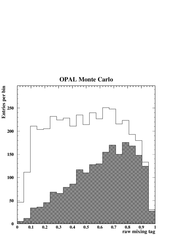
Figure 7: Distribution of the raw mixing tag in simulated signal events. The light histogram shows the distribution of the raw mixing tag, the dark histogram shows the contribution of mixed events.

The deviation of the mixing tag from the $a\,posteriori$ probability is parameterized with the parameters $\alpha_{\mathrm{m}ix}$ and $\beta_{\mathrm{m}ix}$ (used in the oscillation fit Section 7), which quantify the deviations at $x=0.75$ and $x=1.0$ respectively. The resulting fit is shown in Figure 8, and the fitted uncertainty is treated as a systematic error.

Figure 8: Deviation of mixing tag from a true probability. The points with the error bars show simulated events, the solid line is a fit to these points as described in the text and the dotted line is $M=x$, representing a true probability requiring no correction. The error bars include systematic errors described in Section 9. Both charge conjugated cases were added to maximize the statistical significance.

6.3.1 Mixing tag behavior in the combinatorial background

To calculate the likelihood of an event originating from combinatorial background, we need to know the behavior of the mixing tag in combinatorial background events. Two effects which influence this behavior were found using Monte Carlo: a different mixing tag distribution, and oscillations of the background. These effects were identified in particular subsamples of the combinatorial background. The definition, abundance and behavior of those subsamples are as follows.

Combinatorial background events which originated in $\mathrm{b\bar{b}}$ events can exhibit oscillatory behavior if the decaying meson is a $\mathrm{B_{d}}$ or a $\mathrm{B_{s}}$. Two rates of oscillation were found in simulated combinatorial background events:

Oscillation with the same rate as the simulated signal oscillation rate arises primarily when the decay is truly through a $\mathrm{B_{s}}$ and only one of the $\mathrm{D_{s}^{-}}$ decay products is misidentified. The proper decay time reconstruction for these simulated events was less accurate than for signal events, the width (RMS) of the difference between the true time and the expectation value of the reconstructed time distribution is bigger by $25\pm 7\%$ for those events. The mixing tag for these simulated events was essentially the same as for simulated signal events.

It was found that oscillation with the same rate as the $\mathrm{B_{d}}$ oscillation rate arises primarily when the decay products of a $\mathrm{D}^{+}$ or $\mathrm{D}^{0}$ meson produced from a $\mathrm{B_{d}}$ were reconstructed as a $\mathrm{D_{s}^{-}}$ meson, and at most one of the D meson decay products was misidentified. A typical decay chain for this channel is $\mbox{$\mathrm{B_{d}}$}\to\mathrm{D}^{(*)}\ell^{+}\nu\mathrm{(X)}$, which is similar to the signal decay $\mbox{$\mathrm{B_{s}}$}\to\mathrm{D}_{s}\ell^{+}\nu\mathrm{(X)}$. The mixing tag performance and decay time reconstruction for these simulated events were consistent with that for simulated signal events.

Monte Carlo studies have shown that the fraction, $C$, of combinatorial background which oscillates depends on whether the channel contains a $\phi$, both for $\mathrm{B_{s}}$ and $\mathrm{B_{d}}$ fractions. Therefore we use four parameters in the fit, $C_{0}^{\phi}$, $C_{0}^{\mathrm{n}o~{}\phi}$, $C_{s}^{\phi}$ and $C_{s}^{\mathrm{n}o~{}\phi}$, that give the $\mathrm{B_{s}}$ and $\mathrm{B_{d}}$ fractions for $\phi$ and No-$\phi$ channels.

The distribution of the mixing tag for the non-oscillating combinatorial background is different from that for signal, hence the mixing tag not only indicates mixing but also contributes information as to whether the event is a signal event. Our use of this information is described in Section 6.3.2.

Biases were found mainly on non-$\mathrm{b\bar{b}}$ events. While uds events tend to be tagged as mixed, heavier flavor events have a statistically significant tendency to be tagged as unmixed. These tendencies partially cancel out, leaving an overall bias of the mixing tag on non-oscillating combinatorial background events that was found to be $B^{\mathrm{c}omb}_{\mathrm{b}ias}=-0.030\pm 0.009$.

6.3.2 Mixing tag behavior in the $\boldsymbol{\mbox{$\mathrm{D_{s}^{-}}$}\ell^{+}}$ background

The mixing tag for simulated $\mbox{$\mathrm{D_{s}^{-}}$}\ell^{+}$ background events of type (a) (as defined in Section 4.2.1) was essentially opposite that for simulated signal events, as expected from the decay chain. In addition, the distribution of the mixing tag for $\mbox{$\mathrm{D_{s}^{-}}$}\ell^{+}$ background from $\mathrm{B_{u}}$ decay was found to be different from that for signal, while for $\mbox{$\mathrm{D_{s}^{-}}$}\ell^{+}$ background from $\mathrm{B_{d}}$ decay the distribution of the mixing tag was consistent with that for signal. Hence the mixing tag not only indicates mixing, but also contributes information as to whether the event is from the signal, from the combinatorial background (Section 6.3.1), or from the $\mbox{$\mathrm{B_{u}}$}\to\mbox{$\mathrm{D_{s}^{-}}$}\ell^{+}$ background. We derived a probability, $f^{\rm{mix}}_{i}$, given only the mixing tag, that an event is from the combinatorial background, and similarly a probability, $f^{\rm{phys}}_{i}$, that it is from the $\mbox{$\mathrm{B_{u}}$}\to\mbox{$\mathrm{D_{s}^{-}}$}\ell^{+}$ background. Using simulated events we fitted $f^{\rm{mix}}_{i}$ and $f^{\rm{phys}}_{i}$ as functions of the mixing tag, and the fitted uncertainties were used as a systematic uncertainties.

7 Oscillation fit

The likelihood, ${\cal L}$, for observing a particular decay length, $l_{i}$, of candidate $i$, and a particular mixing tag, $M_{i}$, may be parameterized in terms of the candidate’s decay length error, $\sigma^{l}_{i}$, its calculated $\mathrm{B_{s}}$ momentum spectrum (Section  5.2), ${\cal B}_{i}$, and a probability, $f^{\rm{mass}}_{i}$, that it arises from combinatorial background. $f^{\rm{mass}}_{i}$ is determined as a function of the observed invariant mass of this candidate from the fit to the invariant mass spectrum shown in Figure 1.

An event’s likelihood is found by summing over all the possible event types (i.e. signal, the two $\mbox{$\mathrm{D_{s}^{-}}$}\ell^{+}$ background modes, the two oscillating combinatorial background modes, and regular combintorial background). For each event type we assign a probability that it is an event of this type, ${{\mathrm{P}}}({\mathrm{t}ype})$, and the likelihood if the event is of that type, ${\cal L}_{i}^{\mathrm{t}ype}$:

$${\cal L}_{i}(l_{i},M_{i}\mid\sigma^{l}_{i},{\cal B}_{i},f^{\rm{mass}}_{i})=\sum_{\mathrm{e}vent\ type}{{\mathrm{P}}}\Big{(}{\mathrm{t}ype}\Big{|}f^{\rm{comb}}_{i}(f^{\rm{mass}}_{i},f^{\rm{mix}}_{i}),f^{\rm{phys}}_{i}\Big{)}\cdot{{\cal L}_{i}^{\mathrm{t}ype}}(l_{i},M_{i}\mid\sigma^{l}_{i},{\cal B}_{i})~{},$$ (10)

where $f^{\rm{comb}}_{i}$ is the estimated probability that the event arises from combinatorial background based on the invariant mass (through $f^{\rm{mass}}_{i}$) and on the mixing tag (through $f^{\rm{mix}}_{i}$), and $f^{\rm{phys}}_{i}$ is the estimated probability, based on the mixing tag, that the event is from the $\mbox{$\mathrm{B_{u}}$}\to\mbox{$\mathrm{D_{s}^{-}}$}\ell^{+}$ background.

The form of the likelihood function for signal events is given by the convolution of three terms: a term describing the probability of the mixing tag and the true decay length given the true momentum, the calculated momentum distribution, and a Gaussian resolution function with width equal to the decay length error (corrected as described in Section 5.1). This can be expressed as:

$${\cal L}_{i}^{\mathrm{s}ignal}(l_{i},M_{i}\mid\sigma^{l}_{i},{\cal B}_{i}) = \int_{0}^{\infty}\mbox{$\mathrm{d}$}l_{{\mathrm{t}rue},i}$$

$$\int_{0}^{\infty}\mbox{$\mathrm{d}$}p_{\mathrm{t}rue}\ \ {\cal G}(l_{i}\mid l_{{\mathrm{t}rue},i},\sigma^{l}_{i})\ \,{\cal B}_{i}(p_{\mathrm{t}rue})\ \,{\cal P}_{\mathrm{s}ignal}(l_{{\mathrm{t}rue},i},M_{i}\mid p_{\mathrm{t}rue})~{},$$

where the function ${\cal G}$ is a Gaussian function that describes the probability to observe a decay length, $l_{i}$, given a true decay length $l_{{\mathrm{t}rue},i}$ and the estimated measurement uncertainty $\sigma^{l}_{i}$. ${\cal B}_{i}(p_{\mathrm{t}rue})$ is the probability of a particular $\mathrm{B_{s}}$ momentum. ${\cal P}$ is the probability for a given $\mathrm{B_{s}}$ to decay at a distance $l_{{\mathrm{t}rue},i}$ from the $e^{+}e^{-}$ interaction vertex with a mixing tag $M_{i}$. This function is given by:

$${\cal P}_{signal}(l_{{\mathrm{t}rue},i},M_{i}\mid p_{\mathrm{t}rue}) = \frac{m_{\mathrm{B}}}{p_{\mathrm{t}rue}}\cdot\frac{\exp(-t/\mbox{$\mathrm{\tau_{B_{s}}}$})}{\mbox{$\mathrm{\tau_{B_{s}}}$}}\cdot$$

$$\left(\frac{1+{\cal A}\cdot\cos(t\Delta m_{\mathrm{s}})}{2}\cdot(1-M_{i})+\frac{1-{\cal A}\cdot\cos(t\Delta m_{\mathrm{s}})}{2}\cdot M_{i}\right)~{},$$

where $\mathrm{\tau_{B_{s}}}$ is the $\mathrm{B_{s}}$ lifetime, ${\cal A}$ is the fitted amplitude of the oscillation [8] and the $\mathrm{B_{s}}$ candidate’s true proper decay time, $t$, is given by Equation 2.

For the $\mbox{$\mathrm{D_{s}^{-}}$}\ell^{+}$ background events from $\mathrm{B_{d}}$ decay, the likelihood is similar except that the $\mathrm{B_{d}}$ lifetime was used to obtain:

$${\cal P}_{\mathrm{o}sc}(l_{{\mathrm{t}rue},i},M_{i}\mid p_{\mathrm{t}rue}) = \frac{m_{\mathrm{B}}}{p_{\mathrm{t}rue}}\cdot\frac{\exp(-t/\tau_{\mathrm{B_{d}}})}{\tau_{\mathrm{B_{d}}}}\cdot$$ (13)

$$\left(\frac{1+\cos(t\Delta m_{\mathrm{d}})}{2}\cdot(1-M_{i})+\frac{1-\cos(t\Delta m_{\mathrm{d}})}{2}\cdot M_{i}\right)~{},$$

where for decay mode (a) we need to replace $M_{i}$ with $1-M_{i}$. For the $\mbox{$\mathrm{D_{s}^{-}}$}\ell^{+}$ background events from $\mathrm{B_{u}}$ decay, the likelihood is simpler, and contains an exponential decay term with the $\mathrm{B_{u}}$ lifetime weighted by the candidate’s probability to be unmixed.

The combinatorial background was divided into several types according to oscillatory behavior, with most of the combinatorial background events being of the non-oscillating type. The function used to parameterize the reconstructed decay length distribution of this background is the sum of a positive and a negative exponential, convoluted with the same boost function as the signal and a Gaussian resolution function. This can be expressed as:

$${\cal P}_{comb}(l_{i}\mid\tau_{\rm bg}^{+},\tau_{\rm bg}^{-},f_{\rm bg}^{+},p_{\mathrm{t}rue})=\left\{\begin{array}[]{ll}f_{\rm bg}^{+}\,\frac{m_{\mathrm{B}}}{\tau_{\rm bg}^{+}p_{\mathrm{t}rue}}\,\exp\left[\frac{-\,l_{i}\cdot m_{\mathrm{B}}}{\tau_{\rm bg}^{+}p_{\mathrm{t}rue}}\right]&\textrm{if $l_{i}\geq 0$}\\ (1-f_{\rm bg}^{+})\,\frac{m_{\mathrm{B}}}{\tau_{\rm bg}^{-}p_{\mathrm{t}rue}}\,\exp\left[\frac{-\,(-l_{i})\cdot m_{\mathrm{B}}}{\tau_{\rm bg}^{-}p_{\mathrm{t}rue}}\right]&\textrm{if $l_{i}<0$}~{}.\end{array}\right.$$ (14)

The fraction of background with positive lifetime, $f_{\rm bg}^{+}$, as well as the characteristic positive and negative lifetimes of the background, $\tau_{\rm bg}^{+}$ and $\tau_{\rm bg}^{-}$, were obtained from a fit to the sideband region. The resulting value and their uncertainties were used to constrain the background lifetime parameters in the oscillation fit. The background parameters were fitted separately for the hadronic and semileptonic $\mathrm{D_{s}^{-}}$ decay channels, as in [7]. The lifetime behavior of the hadronic $\mathrm{D_{s}^{-}}$ decay channels’ sidebands was best described by fitting only a positive exponential decay. The lifetime behavior of the semileptonic $\mathrm{D_{s}^{-}}$ decay channel’s sideband was best described by fitting both exponential terms.

For the semileptonic channels, the background which include a real $\phi$ not from a $\mathrm{D_{s}^{-}}$ is treated as combinatorial background. For the oscillating types of combinatorial background we used the following: for background oscillating at the $\mathrm{B_{d}}$ frequency we used Equation 13, while for background oscillating at the $\mathrm{B_{s}}$ frequency we used Equation 7.

8 Results of oscillation fit

The results of the amplitude fit to the selected events are shown in Figure 9, including the systematic uncertainties (Section 9). An amplitude peak is evident at $\Delta m_{\mathrm{s}}=6.0\mbox{$\mathrm{\,ps}$}^{-1}$, above the experimental sensitivity, but nevertheless it seems inconsistent with an amplitude of zero with a significance of 2.35 sigma (including systematic uncertainties). The current combined world lower limit is $\Delta m_{\mathrm{s}}>14.4\mbox{$\mathrm{\,ps}$}^{-1}$; this leads us to interpret this peak as a statistical fluctuation. At low frequencies the fitted amplitude quickly rises above the $A=0$ line, and therefore after taking into account all systematic uncertainties described in Section 9, this analysis can only set a weak lower limit of $\Delta m_{\mathrm{s}}>1.0\mbox{$\mathrm{\,ps}$}^{-1}$ at the 95% confidence level.

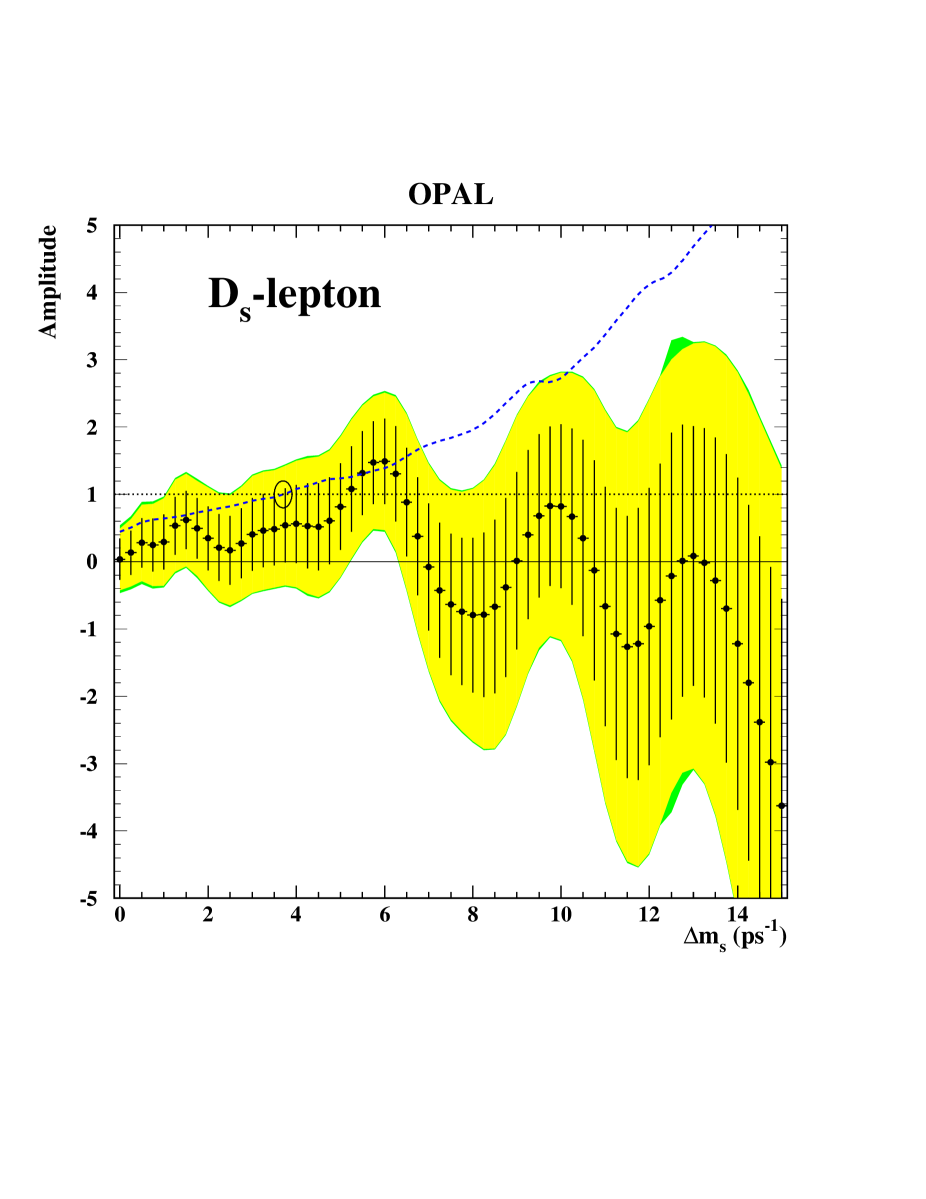
Figure 9: Measured $\mathrm{B_{s}}$ oscillation amplitude as a function of $\Delta m_{\mathrm{s}}$ for this analysis. The error bars represent the 1$\sigma$ statistical uncertainties. The shaded bands show the $\pm 1.645\sigma$ region, with and without including systematic effects. The values of $\Delta m_{\mathrm{s}}$ where the shaded region lies below the ${\cal A}=1$ line are excluded at the 95% confidence level. The dashed line is 1.645$\sigma$ used to determine the experimental sensitivity, which is indicated by the circle.

9 Systematic uncertainties

The systematic uncertainties on the $\mathrm{B_{s}}$ oscillation amplitude, $\sigma^{\mathrm{systematic}}$, are calculated, using the prescription of [8], as:

$$\sigma^{\mathrm{systematic}}={\cal A}^{\mathrm{new}}-{\cal A}^{\mathrm{nominal}}+(1-{\cal A}^{\mathrm{nominal}})\frac{\sigma^{\mathrm{new}}-\sigma^{\mathrm{nominal}}}{\sigma^{\mathrm{nominal}}},$$ (15)

where the superscript “nominal” refers to the amplitude value, ${\cal A}$, and statistical uncertainty, $\sigma$, obtained using the nominal values of the various parameters, and the “new” refers to the new values obtained when a single parameter is increased or decreased by its uncertainty and the fit is repeated. The systematics shown are an average of the effects of the increment and the decrement. The nominal values and errors used are given in Table 2, their description follows:

$\mbox{$\mathrm{D_{s}^{-}}$}\ell^{+}$ background fraction:

The fractions of the two modes of $\mbox{$\mathrm{D_{s}^{-}}$}\ell^{+}$ background out of events in the signal peak (in the case of the semileptonic $\mathrm{D_{s}^{-}}$ decay channel it is done after subtraction of $f_{\mathrm{o}ther}$), $Y^{a}$, $Y^{b}$, and the fraction of $\mathrm{B_{d}}$ decays in each mode, $f_{d}^{a}$ and $f_{d}^{b}$ were calculated in Section 4.2.1. Due to the dependance of $Y^{a}$ and $Y^{b}$ on the $\mathrm{B_{s}}$ production fraction $f_{s}$, the uncertainty on the value of $f_{s}$ is a source of systematic uncertainty.

B meson lifetimes, oscillation and production fractions:

The world averages [1] for the lifetime of the $\mathrm{B_{u}}$, $\mathrm{B_{d}}$ and $\mathrm{B_{s}}$ mesons, for the $\mathrm{B_{d}}$ oscillation frequency and for the $\mathrm{B_{s}}$ production fraction were used.

Oscillating combinatorial background fractions:

The fractions of both types of oscillating combinatorial background out of the total combinatorial background for the various $\mathrm{D_{s}^{-}}$ decay channels: $C_{0}^{\phi}$,$C_{0}^{\mathrm{n}o~{}\phi}$,$C_{s}^{\phi}$ and $C_{s}^{\mathrm{n}o~{}\phi}$ were calculated in Section 6.3.1.

Other background fraction:

The fraction of other types of background specific to semileptonic $\mathrm{D_{s}^{-}}$ decays out of events in the signal peak: $f_{\mathrm{o}ther}$ was estimated as described in Section 4.2.2.

Combinatorial background lifetime:

The combinatorial background parameters
$f_{\rm bg,\thinspace lep}^{+}$, $\tau_{\mathrm{b}g,\thinspace lep}^{+}$ and $\tau_{\mathrm{b}g,\thinspace lep}^{-}$ for semileptonic $\mathrm{D_{s}^{-}}$ decays; and $\tau_{\mathrm{b}g,\thinspace had}^{+}$ for hadronic $\mathrm{D_{s}^{-}}$ decays, were obtained from a fit to sideband events (Section 7). The statistical errors on the parameters from the sideband fit were used as systematic uncertainties.

Mixing tag behavior in signal events:

The uncertainties on the fraction of mixed events in each bin used to parameterize the deviation of the mixing tag from a true probability (as described in section 6.3 and shown in Figure 8) include both statistical uncertainties from the limited Monte Carlo sample size, typically of order 0.025, and the following systematic effects:

• the effect of a one standard deviation variation in the $Q_{\mathrm{s}ame}$ offset, typically of order 0.004.

• the effect of a one standard deviation variation in the $Q_{\mathrm{o}pp}$ offset, typically of order 0.005.

• the effect of a one standard deviation variation in the fragmentation kaon tag’s purity, typically of order 0.007.

• the effect of a one standard deviation variation in the opposite lepton tag’s purity, typically of order 0.006.

• since the limited candidate sample size in data prevents us from showing that the simulation and data agree on the jet charge distributions with and without a fragmentation kaon tag, we take the entire effect of using those distributions instead of the single jet charge distribution as a systematic error, typically of the order of 0.03.

The fitted uncertainties on the deviation parameters $\alpha_{\mathrm{m}ix}$ and $\beta_{\mathrm{m}ix}$ were taken as the systematic uncertainties on the mixing tag.

Mixing tag behavior in background:

The fitted uncertainties on the deviations of the distributions of the mixing tag in combinatorial and $\mbox{$\mathrm{B_{u}}$}\to\mbox{$\mathrm{D_{s}^{-}}$}\ell^{+}$ backgrounds, relative to its behavior in signal (Section 6.3.2), were taken as additional systematic uncertainties.

Decay length error correction:

The fitted uncertainty on the decay length error correction (Section 5.1) was used as a systematic uncertainty.

Decay time reconstruction bias:

The fitted uncertainties on the residual bias in the decay time reconstruction (Section 5.3) were used as systematic uncertainties.

Detector resolution modelling:

The resolution of the tracking detectors might affect the decay time reconstruction and the mixing tag. The simulated resolutions were degraded by $10\thinspace\%$ relative to the values that optimally describe the data following the studies in [18]. The analysis was repeated and the mixing tag was found to be insensitive to this variation while the proper decay time resolution deteriorated by $5\thinspace\%$. This $5\thinspace\%$ uncertainty on the proper decay time resolution was used as a bidirectional systematic uncertainty.

input	nominal		contribution to $\Delta{\cal A}$ at $\Delta m_{\mathrm{s}}$ =
parameter	value	error	$0~{}\mbox{$\mathrm{\,ps}$}^{-1}$	$5~{}\mbox{$\mathrm{\,ps}$}^{-1}$	$10~{}\mbox{$\mathrm{\,ps}$}^{-1}$	$15~{}\mbox{$\mathrm{\,ps}$}^{-1}$
Fractions of $\mbox{$\mathrm{D_{s}^{-}}$}\ell^{+}$ background:
$Y^{a}$	0.143	0.050	+0.09	+0.06	+0.09	+0.11
$f_{d}^{a}$	0.619	0.045	$+0.0011$	+0.0019	+0.004	+0.005
$Y^{b}$	0.065	0.035	$-0.010$	+0.030	$-0.009$	$-0.033$
$f_{d}^{b}$	0.470	0.038	+0.0019	$-0.0010$	$-0.027$	+0.0013
Previously measured B meson properties:
$f_{s}$	0.107	0.014	$-0.030$	$-0.028$	$-0.03$	$-0.030$
$\tau_{\mathrm{B_{u}}}$	$1.653\mbox{$\mathrm{\,ps}$}$	$0.028\mbox{$\mathrm{\,ps}$}$	+0.0005	$-0.0004$	$-0.013$	$-0.0013$
$\tau_{\mathrm{B_{d}}}$	$1.548\mbox{$\mathrm{\,ps}$}$	$0.032\mbox{$\mathrm{\,ps}$}$	+0.0021	+0.0001	$-0.004$	+0.0008
$\mathrm{\tau_{B_{s}}}$	$1.493\mbox{$\mathrm{\,ps}$}$	$0.062\mbox{$\mathrm{\,ps}$}$	$-0.004$	+0.004	+0.016	$-0.04$
$\Delta m_{\mathrm{d}}$	$0.472\mbox{$\mathrm{\,ps}$}^{-1}$	$0.017\mbox{$\mathrm{\,ps}$}^{-1}$	+0.0009	+0.0004	$-0.0002$	$-0.0002$
Fractions of oscillating combinatorial background:
$C_{0}^{\phi}$	0.163	0.030	$-0.0033$	$-0.004$	$-0.015$	$-0.018$
$C_{0}^{\mathrm{n}o~{}\phi}$	0.270	0.027	$-0.005$	+0.0032	+0.0002	+0.008
$C_{s}^{\phi}$	0.163	0.030	$-0.004$	$-0.017$	$-0.022$	$-0.05$
$C_{s}^{\mathrm{n}o~{}\phi}$	0.049	0.013	$-0.0029$	+0.007	+0.010	+0.04
Fraction of other background:
$f_{\mathrm{o}ther}$	0.135	0.057	+0.006	+0.013	+0.010	+0.05
Combinatorial background lifetime fit:
$f_{\rm bg,\thinspace lep}^{+}$	0.92	0.05	+0.0020	+0.0024	$-0.0016$	+0.011
$\tau_{\mathrm{b}g,\thinspace lep}^{+}$	$1.40\mbox{$\mathrm{\,ps}$}$	$0.26\mbox{$\mathrm{\,ps}$}$	+0.0018	$-0.005$	$-0.022$	$-0.04$
$\tau_{\mathrm{b}g,\thinspace lep}^{-}$	$0.7\mbox{$\mathrm{\,ps}$}$	$0.5\mbox{$\mathrm{\,ps}$}$	$-0.0013$	$-0.007$	$-0.012$	$-0.024$
$\tau_{\mathrm{b}g,\thinspace had}^{+}$	$0.70\mbox{$\mathrm{\,ps}$}$	$0.11\mbox{$\mathrm{\,ps}$}$	+0.014	+0.011	$-0.04$	+0.06
Mixing tag behavior in signal events:
$\alpha_{\mathrm{m}ix}$	$-0.006$	0.012	$-0.06$	$-0.024$	+0.021	+0.005
$\beta_{\mathrm{m}ix}$	$-0.051$	0.026	$-0.04$	$-0.06$	$-0.08$	$-0.06$
Mixing tag distributions in background:
combinatorial	1	0.18	$-0.017$	+0.0033	$\phantom{-}0$	$-0.04$
$\mbox{$\mathrm{B_{u}}$}\to\mbox{$\mathrm{D_{s}^{-}}$}\ell^{+}$	1	0.14	$-0.007$	+0.0023	$-0.0023$	$-0.011$
Decay length resolution:
fitted correction	1.478	0.033	+0.0009	+0.016	$-0.005$	+0.06
detector modelling	1	0.05	+0.0012	+0.035	$-0.010$	+0.14
Decay time bias:
$t_{\rm bias}^{0}$	$-0.033\mbox{$\mathrm{\,ps}$}$	$0.005\mbox{$\mathrm{\,ps}$}$	+0.0008	$-0.006$	+0.031	+0.33
$t_{\rm bias}^{\rm slope}$	1.29	0.16	+0.0010	$-0.005$	+0.009	+0.07
systematic uncertainty			0.12	0.11	0.15	0.41
statistical uncertainty			0.28	0.64	1.2	3.0

Table 2: Input parameters for the fit and their contributions to the systematic errors, as described in the text. Systematic errors of less than $5\cdot 10^{-5}$ are reported as zero. For comparison the total systematic errors and the statistical errors are given as well, in the last rows.

The relative importance of the various systematic uncertainties, as a function of $\Delta m_{\mathrm{s}}$, is shown in Table 2. For all $\Delta m_{\mathrm{s}}$ values, the total systematic uncertainty is small compared to the statistical uncertainty. At low $\Delta m_{\mathrm{s}}$ the most important systematic contributions are from the uncertainties on the behavior of the mixing tag in the signal, while at high $\Delta m_{\mathrm{s}}$ the most important systematic contributions are from the uncertainties on the decay time reconstruction bias.

10 Checks of the method

10.1 Fitted decay length distribution and lifetime fit

The form of the likelihood of a candidate decaying with a measured decay length $l_{i}$ has been stated in Section 7. By setting the various parameters to their nominal values and the amplitude to zero, we acquired a prediction for the distribution of $l_{i}$. This prediction compared well with the actual measured values of $l_{i}$, as shown in Figure 10.

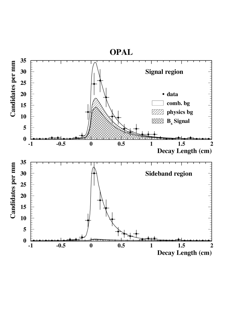
Figure 10: Comparison of expectation from fit results and actual decay length distributions. The fit results are shown by the curves, with individual components shaded, while the decay lengths measured in the data are shown by the error bars. The sideband region was used in the combinatorial background lifetime fit.

The likelihood can also be used to measure the $\mathrm{B_{s}}$ lifetime by ignoring the mixing tag and fitting the $\mathrm{B_{s}}$ lifetime to the data. The resulting lifetime is $1.57\pm 0.17\mbox{$\mathrm{\,ps}$}$, which is consistent with the world average value of $1.54\pm 0.07\mbox{$\mathrm{\,ps}$}$.

10.2 Oscillation fit on simulated events

A likelihood fit for $\Delta m_{\mathrm{s}}$ was performed on a simulated Monte Carlo event sample having the same statistics and estimated composition as the data, with an oscillation at a true frequency of either $\Delta m_{\mathrm{s}}=2.0\mbox{$\mathrm{\,ps}$}^{-1}$ or $\Delta m_{\mathrm{s}}=3.0\mbox{$\mathrm{\,ps}$}^{-1}$. The fit yielded $\Delta m_{\mathrm{s}}=1.98^{+0.15}_{-0.14}\mbox{$\mathrm{\,ps}$}^{-1}$ and $\Delta m_{\mathrm{s}}=3.16^{+0.26}_{-0.23}\mbox{$\mathrm{\,ps}$}^{-1}$ respectively, in agreement with the input values. Performing an amplitude fit (ignoring systematic uncertainties) on the same Monte Carlo events yielded the results shown in Figure 11. As expected, the amplitude is consistent with $1$ at the true value of $\Delta m_{\mathrm{s}}$.

The sensitivity of the analysis is defined as the expected highest oscillation frequency excluded at the 95% confidence level, given that the true $\Delta m_{\mathrm{s}}$ is infinitely high. Given an infinitely high $\Delta m_{\mathrm{s}}$ the expectation value of the amplitude at all fitted values of $\Delta m_{\mathrm{s}}$ is zero [8]. This allows us to evaluate the sensitivity as the frequency at which the resulting $1.645\sigma$ line rises above an amplitude of one, as shown in Figure 9. The experimental sensitivity of this analysis is $4.1\mbox{$\mathrm{\,ps}$}^{-1}$.

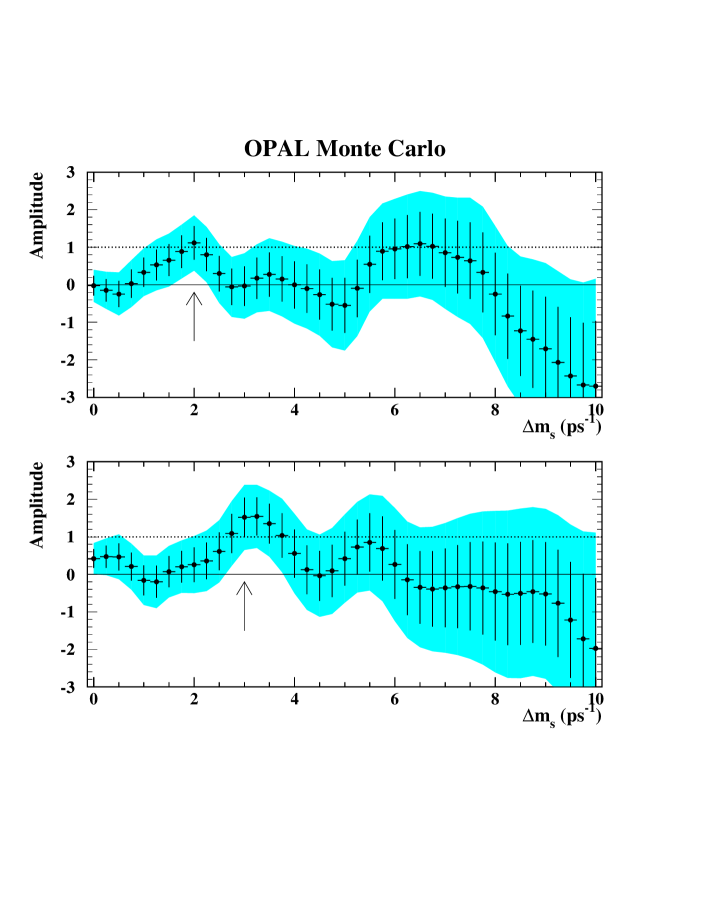
Figure 11: Measured $\mathrm{B_{s}}$ oscillation amplitude as a function of $\Delta m_{\mathrm{s}}$ in simulated events with a true $\Delta m_{\mathrm{s}}$ of $2.0\mbox{$\mathrm{\,ps}$}^{-1}$ in the upper plot, and $3.0\mbox{$\mathrm{\,ps}$}^{-1}$ in the lower plot. The error bars represent the 1$\sigma$ statistical uncertainties. The shaded bands show the $\pm 1.645\sigma$ region (systematic effects not included). The arrows point at the simulated value of $\Delta m_{\mathrm{s}}$.

11 Conclusion

A sample of $\mathrm{B_{s}}$ decays obtained using $\mbox{$\mathrm{D_{s}^{-}}$}\ell^{+}$ combinations was used to study $\mathrm{B_{s}}$ oscillation. The estimated sensitivity of the analysis is $4.1\mbox{$\mathrm{\,ps}$}^{-1}$. The resulting, stand-alone, lower limit from our analysis is significantly lower, at $1.0\mbox{$\mathrm{\,ps}$}^{-1}$. This limit is not competitive with existing limits. However, this does not diminish the contribution of this analysis to the world combined measurement, which is at the rapid oscillation region. The previous OPAL measurement [6] was an inclusive measurement, and so has only a negligable statistical correlation with our measurement. Its sensitivity was $6.7\mbox{$\mathrm{\,ps}$}^{-1}$ and it set a lower limit of $5.1\mbox{$\mathrm{\,ps}$}^{-1}$. Combining it with our results we get the combined measurement shown in Figure 12, a sensitivity of $8.0\mbox{$\mathrm{\,ps}$}^{-1}$ and a limit of $5.1\mbox{$\mathrm{\,ps}$}^{-1}$.

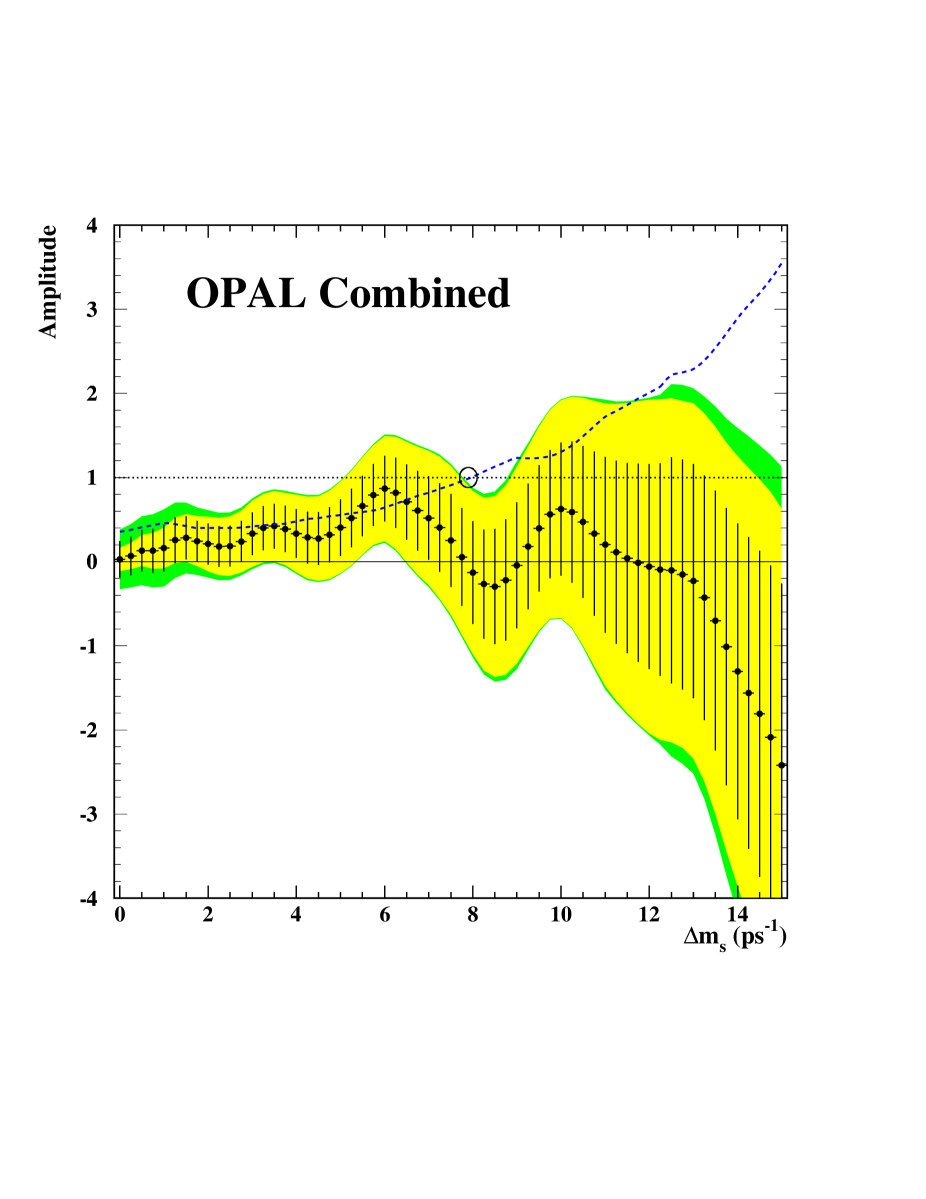
Figure 12: Measured $\mathrm{B_{s}}$ oscillation amplitude as a function of $\Delta m_{\mathrm{s}}$ combined for this analysis and the previous OPAL analysis. The error bars represent the 1$\sigma$ statistical uncertainties. The shaded bands show the $\pm 1.645\sigma$ region, with and without including systematic effects. The values of $\Delta m_{\mathrm{s}}$ where the shaded region lies below the ${\cal A}=1$ line are excluded at the 95% confidence level. The dashed line is 1.645$\sigma$ used to determine the experimental sensitivity, which is indicated by the circle.

12 Acknowledgements

We particularly wish to thank the SL Division for the efficient operation of the LEP accelerator at all energies and for their continuing close cooperation with our experimental group. We thank our colleagues from CEA, DAPNIA/SPP, CE-Saclay for their efforts over the years on the time-of-flight and trigger systems which we continue to use. In addition to the support staff at our own institutions we are pleased to acknowledge the
Department of Energy, USA,
National Science Foundation, USA,
Particle Physics and Astronomy Research Council, UK,
Natural Sciences and Engineering Research Council, Canada,
Israel Science Foundation, administered by the Israel Academy of Science and Humanities,
Minerva Gesellschaft,
Benoziyo Center for High Energy Physics,
Japanese Ministry of Education, Science and Culture (the Monbusho) and a grant under the Monbusho International Science Research Program,
Japanese Society for the Promotion of Science (JSPS),
German Israeli Bi-national Science Foundation (GIF),
Bundesministerium für Bildung und Forschung, Germany,
National Research Council of Canada,
Research Corporation, USA,
Hungarian Foundation for Scientific Research, OTKA T-029328, T023793 and OTKA F-023259.

References

- [1] Particle Data Group, C. Caso et al., Eur. Phys. J. C 3 (1998) 1.
- [2] A. Ali and D. London, Z. Phys. C 65 (1995) 431, and references therein.
- [3] Y. Nir, Phys. Lett. B 327 (1994) 85.
-
[4]
OPAL Collaboration, K. Ackerstaff et al., Z. Phys. C 76 (1997)
401;
OPAL Collaboration, K. Ackerstaff et al., Z. Phys. C 76 (1997) 417;
DELPHI Collab., W. Adam et al., Phys. Lett. B 414 (1997) 382;
CDF Collab., F. Abe et al., Phys. Rev. Lett. 82 (1999) 3576. -
[5]
ALEPH Collaboration, D. Buskulic et al., Phys. Lett. B 377 (1996) 205;
ALEPH Collaboration, R. Barate et al., Eur. Phys. J. C 7 (1999) 553. - [6] OPAL Collab., G. Abbiendi et al., Eur. Phys. J. C 11 (1999) 587.
- [7] OPAL Collab., K. Ackerstaff et al., Phys Lett. B 426 (1998) 161.
- [8] H. G. Moser and A. Roussarie, Nucl. Inst. and Meth. A 384 (1997) 491.
- [9] D. Abbaneo and G. Boix, JHEP 9908, 004 (1999).
-
[10]
OPAL Collab., K. Ahmet et al., Nucl. Instr. and Meth.
A 305 (1991) 275;
OPAL Collab., P. P. Allport et al., Nucl. Instr. and Meth. A 324 (1993) 34;
OPAL Collab., P. P. Allport et al., Nucl. Instr. and Meth. A 346 (1994) 476. - [11] OPAL Collab., G. Alexander et al., Z. Phys. C 52 (1991) 175.
-
[12]
JADE Collab., W. Bartel et al., Z. Phys. C 33 (1986) 23;
JADE Collab., S. Bethke et al., Phys. Lett. B 213 (1988) 235. -
[13]
T. Sjöstrand, Comp. Phys. Comm. 39 (1986) 347;
M. Bengtsson and T. Sjöstrand, Comp. Phys. Comm. 43 (1987) 367;
T. Sjöstrand, Int. J. of Mod. Phys. A 3 (1988) 751;
T. Sjöstrand, Comp. Phys. Comm. 82 (1994) 74. - [14] C. Peterson et al., Phys. Rev. D 27 (1983) 105.
- [15] J. Allison et al., Nucl. Inst. and Meth. A 317 (1992) 47.
- [16] OPAL Collab., R. Akers et al., Z. Phys. C 66 (1995) 19.
- [17] OPAL Collab., R. Akers et al., Phys. Lett. B 316 (1993) 435.
- [18] OPAL Collab., G. Abbiendi et al., Eur. Phys. J. C 8 (1999) 217.
- [19] OPAL Collab., P.D. Acton et al., Z. Phys. C 58 (1993) 523.
-
[20]
OPAL Collab., P.D. Acton et al., Z. Phys. C 59 (1993) 183;
OPAL Collab., R. Akers et al., Phys. Lett. B 338 (1994) 497. - [21] OPAL Collab., G. Abbiendi et al., CERN-EP/2000-065. Accepted by Phys. Lett. B.
- [22] E. Golowich et al., Z. Phys. C 48 (1990) 89.
- [23] OPAL Collab., R. Akers et al., Z. Phys. C 67 (1995) 379.
- [24] OPAL Collab., K. Ackerstaff et al., Eur. Phys. J. C 5 (1998) 379.