A search for resonance decays to $\mkern 1.5mu\overline{\mkern-1.5mu\nu\mkern-1.0mu}\mkern 1.0mu$-jet in $e^{+}p$ scattering at HERA

Abstract

A study of the $\bar{\nu}$-jet mass spectrum in $e^{+}p\rightarrow\bar{\nu}X$ events at center-of-mass energy 300 GeV has been performed with the ZEUS detector at HERA using an integrated luminosity of $47.7\mbox{pb}^{-1}$. The mass spectrum is in good agreement with that expected from Standard Model processes over the $\bar{\nu}$-jet mass range studied. No significant excess attributable to the decay of a narrow resonance is observed. By using both $e^{+}p\rightarrow e^{+}X$ and $e^{+}p\rightarrow\bar{\nu}X$ data, mass-dependent limits are set on the $s$-channel production of scalar and vector resonant states. Couplings to first-generation quarks are considered and limits are presented as a function of the $e^{+}q$ and $\mkern 1.5mu\overline{\mkern-1.5mu\nu\mkern-1.0mu}\mkern 1.0muq$ branching ratios. These limits are used to constrain the production of leptoquarks and $R$-parity violating squarks.

DESY 00-133
September 2000

The ZEUS Collaboration

J. Breitweg, S. Chekanov, M. Derrick, D. Krakauer, S. Magill, B. Musgrave, A. Pellegrino, J. Repond, R. Stanek, R. Yoshida
Argonne National Laboratory, Argonne, IL, USA ^p

M.C.K. Mattingly
Andrews University, Berrien Springs, MI, USA

P. Antonioli, G. Bari, M. Basile, L. Bellagamba, D. Boscherini¹, A. Bruni, G. Bruni, G. Cara Romeo, L. Cifarelli², F. Cindolo, A. Contin, M. Corradi, S. De Pasquale, P. Giusti, G. Iacobucci, G. Levi, A. Margotti, T. Massam, R. Nania, F. Palmonari, A. Pesci, G. Sartorelli, A. Zichichi
University and INFN Bologna, Bologna, Italy ^f

C. Amelung³, A. Bornheim⁴, I. Brock, K. Coböken⁵, J. Crittenden, R. Deffner⁶, H. Hartmann, K. Heinloth⁷, E. Hilger, P. Irrgang, H.-P. Jakob, A. Kappes⁸, U.F. Katz, R. Kerger, E. Paul, J. Rautenberg,
H. Schnurbusch, A. Stifutkin, J. Tandler, K.C. Voss, A. Weber, H. Wieber
Physikalisches Institut der Universität Bonn, Bonn, Germany ^c

D.S. Bailey, O. Barret, N.H. Brook⁹, B. Foster¹, G.P. Heath, H.F. Heath, E. Rodrigues¹⁰, J. Scott, R.J. Tapper
H.H. Wills Physics Laboratory, University of Bristol, Bristol, U.K. ^o

M. Capua, A. Mastroberardino, M. Schioppa, G. Susinno
Calabria University, Physics Dept.and INFN, Cosenza, Italy ^f

H.Y. Jeoung, J.Y. Kim, J.H. Lee, I.T. Lim, K.J. Ma, M.Y. Pac¹¹
Chonnam National University, Kwangju, Korea ^h

A. Caldwell, W. Liu, X. Liu, B. Mellado, S. Paganis, S. Sampson, W.B. Schmidke, F. Sciulli
Columbia University, Nevis Labs., Irvington on Hudson, N.Y., USA ^q

J. Chwastowski, A. Eskreys, J. Figiel, K. Klimek, K. Olkiewicz, K. Piotrzkowski³, M.B. Przybycień, P. Stopa, L. Zawiejski
Inst. of Nuclear Physics, Cracow, Poland ^j

B. Bednarek, K. Jeleń, D. Kisielewska, A.M. Kowal, T. Kowalski, M. Przybycień, E. Rulikowska-Zarȩbska, L. Suszycki, D. Szuba
Faculty of Physics and Nuclear Techniques, Academy of Mining and Metallurgy, Cracow, Poland ^j

A. Kotański
Jagellonian Univ., Dept. of Physics, Cracow, Poland ^k

L.A.T. Bauerdick, U. Behrens, J.K. Bienlein, K. Borras, V. Chiochia, D. Dannheim, K. Desler, G. Drews, A. Fox-Murphy, U. Fricke, F. Goebel, S. Goers, P. Göttlicher, R. Graciani, T. Haas, W. Hain, G.F. Hartner, D. Hasell¹², K. Hebbel, S. Hillert, M. Kasemann¹³, W. Koch¹⁴, U. Kötz, H. Kowalski, H. Labes, L. Lindemann¹⁵, B. Löhr, R. Mankel, J. Martens, M. Martínez, M. Milite, M. Moritz, D. Notz, M.C. Petrucci, A. Polini, M. Rohde⁷, A.A. Savin, U. Schneekloth, F. Selonke, M. Sievers¹⁶, S. Stonjek, G. Wolf, U. Wollmer, C. Youngman, W. Zeuner
Deutsches Elektronen-Synchrotron DESY, Hamburg, Germany

C. Coldewey, A. Lopez-Duran Viani, A. Meyer, S. Schlenstedt, P.B. Straub
DESY Zeuthen, Zeuthen, Germany

G. Barbagli, E. Gallo, A. Parenti, P. G. Pelfer
University and INFN, Florence, Italy ^f

A. Bamberger, A. Benen, N. Coppola, S. Eisenhardt¹⁷, P. Markun, H. Raach, S. Wölfle
Fakultät für Physik der Universität Freiburg i.Br., Freiburg i.Br., Germany ^c

P.J. Bussey, M. Bell, A.T. Doyle, C. Glasman¹⁸, S.W. Lee, A. Lupi, N. Macdonald, G.J. McCance, D.H. Saxon,
L.E. Sinclair, I.O. Skillicorn, R. Waugh
Dept. of Physics and Astronomy, University of Glasgow, Glasgow, U.K. ^o

I. Bohnet, N. Gendner, U. Holm, A. Meyer-Larsen, H. Salehi, K. Wick
Hamburg University, I. Institute of Exp. Physics, Hamburg, Germany ^c

T. Carli, A. Garfagnini, I. Gialas¹⁹, L.K. Gladilin²⁰, D. Kçira²¹, R. Klanner, E. Lohrmann
Hamburg University, II. Institute of Exp. Physics, Hamburg, Germany ^c

R. Gonçalo¹⁰, K.R. Long, D.B. Miller, A.D. Tapper, R. Walker
Imperial College London, High Energy Nuclear Physics Group, London, U.K. ^o

U. Mallik
University of Iowa, Physics and Astronomy Dept., Iowa City, USA ^p

P. Cloth, D. Filges
Forschungszentrum Jülich, Institut für Kernphysik, Jülich, Germany

T. Ishii, M. Kuze, K. Nagano, K. Tokushuku²², S. Yamada, Y. Yamazaki
Institute of Particle and Nuclear Studies, KEK, Tsukuba, Japan ^g

S.H. Ahn, S.B. Lee, S.K. Park
Korea University, Seoul, Korea ^h

H. Lim, I.H. Park, D. Son
Kyungpook National University, Taegu, Korea ^h

F. Barreiro, G. García, O. González, L. Labarga, J. del Peso, I. Redondo²³, J. Terrón, M. Vázquez
Univer. Autónoma Madrid, Depto de Física Teórica, Madrid, Spain ⁿ

M. Barbi, F. Corriveau, D.S. Hanna, A. Ochs, S. Padhi, D.G. Stairs, M. Wing
McGill University, Dept. of Physics, Montréal, Québec, Canada ${}^{a},$  ^b

T. Tsurugai
Meiji Gakuin University, Faculty of General Education, Yokohama, Japan

A. Antonov, V. Bashkirov²⁴, M. Danilov, B.A. Dolgoshein, D. Gladkov, V. Sosnovtsev, S. Suchkov
Moscow Engineering Physics Institute, Moscow, Russia ^l

R.K. Dementiev, P.F. Ermolov, Yu.A. Golubkov, I.I. Katkov, L.A. Khein, N.A. Korotkova,
I.A. Korzhavina, V.A. Kuzmin, O.Yu. Lukina, A.S. Proskuryakov, L.M. Shcheglova, A.N. Solomin, N.N. Vlasov, S.A. Zotkin
Moscow State University, Institute of Nuclear Physics, Moscow, Russia ^m

C. Bokel, M. Botje, N. Brümmer, J. Engelen, S. Grijpink, E. Koffeman, P. Kooijman, S. Schagen, A. van Sighem, E. Tassi, H. Tiecke, N. Tuning, J.J. Velthuis, J. Vossebeld, L. Wiggers, E. de Wolf
NIKHEF and University of Amsterdam, Amsterdam, Netherlands ⁱ

B. Bylsma, L.S. Durkin, J. Gilmore, C.M. Ginsburg, C.L. Kim, T.Y. Ling
Ohio State University, Physics Department, Columbus, Ohio, USA ^p

S. Boogert, A.M. Cooper-Sarkar, R.C.E. Devenish, J. Große-Knetter²⁵, T. Matsushita, O. Ruske,
M.R. Sutton, R. Walczak
Department of Physics, University of Oxford, Oxford U.K. ^o

A. Bertolin, R. Brugnera, R. Carlin, F. Dal Corso, U. Dosselli, S. Dusini, S. Limentani, M. Morandin, M. Posocco, L. Stanco, R. Stroili, M. Turcato, C. Voci
Dipartimento di Fisica dell’ Università and INFN, Padova, Italy ^f

L. Adamczyk²⁶, L. Iannotti²⁶, B.Y. Oh, J.R. Okrasiński, P.R.B. Saull²⁶, W.S. Toothacker¹⁴$\dagger$,
J.J. Whitmore
Pennsylvania State University, Dept. of Physics, University Park, PA, USA ^q

Y. Iga
Polytechnic University, Sagamihara, Japan ^g

G. D’Agostini, G. Marini, A. Nigro
Dipartimento di Fisica, Univ. ’La Sapienza’ and INFN, Rome, Italy ${}^{f}\leavevmode\nobreak\$

C. Cormack, J.C. Hart, N.A. McCubbin, T.P. Shah
Rutherford Appleton Laboratory, Chilton, Didcot, Oxon, U.K. ^o

D. Epperson, C. Heusch, H.F.-W. Sadrozinski, A. Seiden, R. Wichmann, D.C. Williams
University of California, Santa Cruz, CA, USA ^p

N. Pavel
Fachbereich Physik der Universität-Gesamthochschule Siegen, Germany ^c

H. Abramowicz²⁷, S. Dagan²⁸, S. Kananov²⁸, A. Kreisel, A. Levy²⁸
Raymond and Beverly Sackler Faculty of Exact Sciences, School of Physics, Tel-Aviv University, Tel-Aviv, Israel ^e

T. Abe, T. Fusayasu, K. Umemori, T. Yamashita
Department of Physics, University of Tokyo, Tokyo, Japan ^g

R. Hamatsu, T. Hirose, M. Inuzuka, S. Kitamura²⁹, T. Nishimura
Tokyo Metropolitan University, Dept. of Physics, Tokyo, Japan ^g

M. Arneodo³⁰, N. Cartiglia, R. Cirio, M. Costa, M.I. Ferrero, S. Maselli, V. Monaco, C. Peroni, M. Ruspa, R. Sacchi, A. Solano, A. Staiano
Università di Torino, Dipartimento di Fisica Sperimentale and INFN, Torino, Italy ^f

D.C. Bailey, C.-P. Fagerstroem, R. Galea, T. Koop, G.M. Levman, J.F. Martin, R.S. Orr, S. Polenz, A. Sabetfakhri, D. Simmons
University of Toronto, Dept. of Physics, Toronto, Ont., Canada ^a

J.M. Butterworth, C.D. Catterall, M.E. Hayes, E.A. Heaphy, T.W. Jones, J.B. Lane, B.J. West
University College London, Physics and Astronomy Dept., London, U.K. ^o

J. Ciborowski, R. Ciesielski, G. Grzelak, R.J. Nowak, J.M. Pawlak, R. Pawlak, B. Smalska,
T. Tymieniecka, A.K. Wróblewski, J.A. Zakrzewski, A.F. Żarnecki
Warsaw University, Institute of Experimental Physics, Warsaw, Poland ^j

M. Adamus, T. Gadaj
Institute for Nuclear Studies, Warsaw, Poland ^j

O. Deppe, Y. Eisenberg, D. Hochman, U. Karshon²⁸
Weizmann Institute, Department of Particle Physics, Rehovot, Israel ^d

W.F. Badgett, D. Chapin, R. Cross, C. Foudas, S. Mattingly, D.D. Reeder, W.H. Smith, A. Vaiciulis³¹, T. Wildschek, M. Wodarczyk
University of Wisconsin, Dept. of Physics, Madison, WI, USA ^p

A. Deshpande, S. Dhawan, V.W. Hughes
Yale University, Department of Physics, New Haven, CT, USA ^p

S. Bhadra, C. Catterall, J.E. Cole, W.R. Frisken, R. Hall-Wilton, M. Khakzad, S. Menary
York University, Dept. of Physics, Toronto, Ont., Canada ^a

¹ now visiting scientist at DESY
² now at Univ. of Salerno and INFN Napoli, Italy
³ now at CERN
⁴ now at CalTech, USA
⁵ now at Sparkasse Bonn, Germany
⁶ now at Siemens ICN, Berlin, Germanny
⁷ retired
⁸ supported by the GIF, contract I-523-13.7/97
⁹ PPARC Advanced fellow
¹⁰ supported by the Portuguese Foundation for Science and Technology
¹¹ now at Dongshin University, Naju, Korea
¹² now at Massachusetts Institute of Technology, Cambridge, MA, USA
¹³ now at Fermilab, Batavia, IL, USA
¹⁴ deceased
¹⁵ now at SAP A.G., Walldorf, Germany
¹⁶ now at Netlife AG, Hamburg, Germany
¹⁷ now at University of Edinburgh, Edinburgh, U.K.
¹⁸ supported by an EC fellowship number ERBFMBICT 972523
¹⁹ visitor of Univ. of Crete, Greece, partially supported by DAAD, Bonn - Kz. A/98/16764
²⁰ on leave from MSU, supported by the GIF, contract I-0444-176.07/95
²¹ supported by DAAD, Bonn - Kz. A/98/12712
²² also at University of Tokyo
²³ supported by the Comunidad Autonoma de Madrid
²⁴ now at Loma Linda University, Loma Linda, CA, USA
²⁵ supported by the Feodor Lynen Program of the Alexander von Humboldt foundation
²⁶ partly supported by Tel Aviv University
²⁷ an Alexander von Humboldt Fellow at University of Hamburg
²⁸ supported by a MINERVA Fellowship
²⁹ present address: Tokyo Metropolitan University of Health Sciences, Tokyo 116-8551, Japan
³⁰ now also at Università del Piemonte Orientale, I-28100 Novara, Italy
³¹ now at University of Rochester, Rochester, NY, USA

a	supported by the Natural Sciences and Engineering Research Council of Canada (NSERC)
b	supported by the FCAR of Québec, Canada
c	supported by the German Federal Ministry for Education and Science, Research and Technology (BMBF), under contract numbers 057BN19P, 057FR19P, 057HH19P, 057HH29P, 057SI75I
d	supported by the MINERVA Gesellschaft für Forschung GmbH, the German Israeli Foundation, the Israel Science Foundation, the U.S.-Israel Binational Science Foundation, the Israel Ministry of Science and the Benozyio Center for High Energy Physics
e	supported by the German-Israeli Foundation, the Israel Science Foundation, the U.S.-Israel Binational Science Foundation, and by the Israel Ministry of Science
f	supported by the Italian National Institute for Nuclear Physics (INFN)
g	supported by the Japanese Ministry of Education, Science and Culture (the Monbusho) and its grants for Scientific Research
h	supported by the Korean Ministry of Education and Korea Science and Engineering Foundation
i	supported by the Netherlands Foundation for Research on Matter (FOM)
j	supported by the Polish State Committee for Scientific Research, grant No. 112/E-356/SPUB/DESY/P03/DZ 3/99, 620/E-77/SPUB/DESY/P-03/ DZ 1/99, 2P03B03216, 2P03B04616, 2P03B03517, and by the German Federal Ministry of Education and Science, Research and Technology (BMBF)
k	supported by the Polish State Committee for Scientific Research (grant No. 2P03B08614 and 2P03B06116)
l	partially supported by the German Federal Ministry for Education and Science, Research and Technology (BMBF)
m	supported by the Fund for Fundamental Research of Russian Ministry for Science and Education and by the German Federal Ministry for Education and Science, Research and Technology (BMBF)
n	supported by the Spanish Ministry of Education and Science through funds provided by CICYT
o	supported by the Particle Physics and Astronomy Research Council
p	supported by the US Department of Energy
q	supported by the US National Science Foundation

1 Introduction

A number of extensions of the Standard Model of elementary particles predict the existence of electron-quark resonant states at high mass. Such states include leptoquarks (LQs) [1] and $R$-parity violating (${\not{R}_{p}}$) squarks [2]. The corresponding production processes could give a large cross section for high-mass $\mkern 1.5mu\overline{\mkern-1.5mu\nu\mkern-1.0mu}\mkern 1.0mu$-jet or $e^{+}$-jet events.

This paper presents an analysis of the ZEUS data aimed at searching for high-mass scalar and vector resonant states decaying into an antineutrino plus a jet. A similar search in the $e^{+}$-jet final states with the ZEUS data was published previously [3]. To avoid the constraints from a specific model, minimal assumptions are made about the properties of the resonant state.

This analysis uses events whose observed final state has large missing transverse momentum and at least one jet. These event characteristics correspond to an outgoing antineutrino and a scattered quark in $e^{+}p\rightarrow\mkern 1.5mu\overline{\mkern-1.5mu\nu\mkern-1.0mu}\mkern 1.0muX$ scattering. The data-selection and event-reconstruction techniques are similar to those used for measuring the charged current (CC) cross section [4]. The $\mkern 1.5mu\overline{\mkern-1.5mu\nu\mkern-1.0mu}\mkern 1.0mu$-jet invariant mass is calculated from the energies and angles of the final-state antineutrino and jet:

$$M_{\nu j}^{2}=2E_{\nu}E_{jet}(1-\cos\xi)$$ (1)

where $E_{\nu}$ and $E_{jet}$ are the energies of the scattered antineutrino and jet (assumed massless), respectively. The angle $\xi$ is the laboratory-frame opening angle between the jet and the antineutrino. Since the antineutrino escapes detection, its momentum is deduced from all observed final-state particles by assuming conservation of energy-momentum in the event.

In the following sections, the expectations of antineutrino-jet final states from the Standard Model (SM) and from models that predict resonant states are first reviewed. After a summary of experimental conditions and data selection, the analysis is described and the reconstructed mass spectrum is presented. Since there is no evidence for a narrow resonance in either the $\mkern 1.5mu\overline{\mkern-1.5mu\nu\mkern-1.0mu}\mkern 1.0mu$-jet or the previously published $e^{+}$-jet mass spectra, limits are set on the production of positron-quark resonant states using both data sets. The application of these limits to LQ and squark production is then discussed.

2 Signal and background expectations

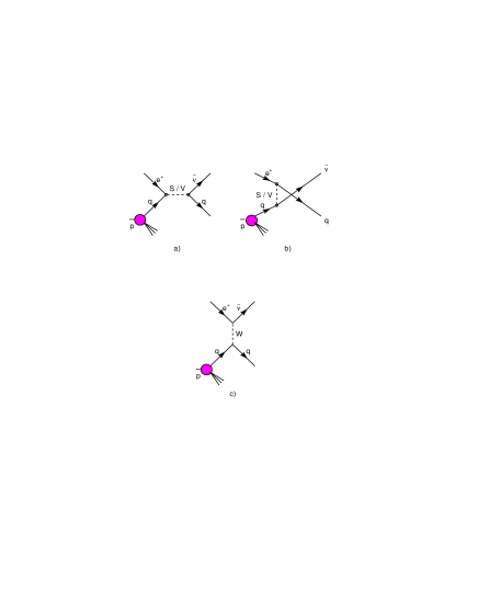
Figure 1: Processes with $\mkern 1.5mu\overline{\mkern-1.5mu\nu\mkern-1.0mu}\mkern 1.0mu$-jet final states in $e^{+}p$ collisions. A scalar (S) or vector (V) intermediate state can be formed via a) $s$-channel or b) $u$-channel exchange. Weak charged current scattering c) forms the primary background to these processes.

High-mass $\mkern 1.5mu\overline{\mkern-1.5mu\nu\mkern-1.0mu}\mkern 1.0mu$-jet final states can be formed either through SM mechanisms or via processes that produce lepton-quark resonances. Figure 1 shows scattering mechanisms producing such final states in $e^{+}p$ collisions. The CC scattering mechanism shown in Fig. 1c forms the primary background in this search. Neutral current (NC) and photoproduction processes form negligible backgrounds since neither produces events with a large observed final-state momentum imbalance.

2.1 Standard Model expectations

The kinematic variables used to describe the process $e^{+}p\rightarrow\mkern 1.5mu\overline{\mkern-1.5mu\nu\mkern-1.0mu}\mkern 1.0muX$ are:

$$Q^{2} =-q^{2}=-(k-k^{\prime})^{2}$$ (2)

$$x =\frac{Q^{2}}{2P\cdot q}$$ (3)

$$y =\frac{q\cdot P}{k\cdot P}$$ (4)

where $P$ is the four-momentum of the incoming proton, and $k$ and $k^{\prime}$ are the four-momenta of the incoming positron and the outgoing antineutrino, respectively. These variables are related by $Q^{2}=sxy$. The quantity $x$ is interpreted as the fraction of the proton momentum carried by the struck quark, and $y$ measures the fractional energy transferred by the $W$ in the CC process.

Assuming no QED or QCD radiation, the mass of the $\mkern 1.5mu\overline{\mkern-1.5mu\nu\mkern-1.0mu}\mkern 1.0muq$ system is related to $x$ via

$$M^{2}=sx$$ (5)

and the scattering angle, $\theta^{\ast}$, of the outgoing antineutrino relative to the beam positron, as viewed in the $\mkern 1.5mu\overline{\mkern-1.5mu\nu\mkern-1.0mu}\mkern 1.0muq$ center-of-mass system, is related to $y$ via

$$\cos\theta^{\ast}=1-2y\;.$$ (6)

In leading-order electroweak theory, the CC cross section can be expressed as:

$$\frac{d^{2}\sigma^{CC}(e^{+}p)}{dxdy}=\frac{sG_{F}^{2}}{4\pi}\left(\frac{M_{W}^{2}}{M_{W}^{2}+xys}\right)^{2}\left[Y_{+}F^{CC}_{2}-Y_{-}xF^{CC}_{3}-y^{2}F^{CC}_{L}\right]$$ (7)

where $G_{F}$ is the Fermi constant, $M_{W}$ is the mass of the $W$ boson, and $Y_{\pm}=1\pm(1-y)^{2}$.  The proton structure functions $F_{2}^{CC}$ and $xF_{3}^{CC}$, in leading-order (LO) QCD, measure respectively sums and differences of quark and antiquark parton momentum densities [5]. The longitudinal structure function, $F_{L}^{CC}$, contributes negligibly to this cross section except at $y$ near 1 [4].  In the region of high mass ($x\rightarrow 1$) the structure functions $F_{2}^{CC}$ and $xF_{3}^{CC}$ are dominated by the valence quark distributions in the proton.  For $e^{+}p$ collisions, the scattering from down quarks dominates the cross section. The CC cross section peaks at small $y$, which leads to a $\cos\theta^{\ast}$ distribution rising toward $\cos\theta^{\ast}=1$.

The largest uncertainty in the CC cross-section prediction arises from the parton densities of the proton. The parton density functions (PDF) are parameterizations which, at high $x$, are determined primarily from measurements made in fixed-target deep inelastic scattering (DIS) experiments. In the high-mass range ($x\approx 0.6$ corresponding to a $\mkern 1.5mu\overline{\mkern-1.5mu\nu\mkern-1.0mu}\mkern 1.0mu$-jet mass of $230\,\mbox{GeV}$), the PDFs introduce an uncertainty of $\approx 25\%$ in the predicted $e^{+}p$ CC cross section [6]. It should be noted that recent studies of PDFs suggest that the $d$-quark density in the proton has been systematically underestimated for $x>0.3$ [6, 7, 8, 9]. As an example, Yang and Bodek [8] propose a correction to the $d/u$ quark density ratio in the MRS(R2) PDF [10]:

$$\delta\left(\frac{d}{u}\right)=0.1x(x+1)$$ (8)

which fits the available data better.  When this correction is applied to the CTEQ4D PDFs [11], the increase in the predicted CC cross section (and the corresponding number of high-mass $\mkern 1.5mu\overline{\mkern-1.5mu\nu\mkern-1.0mu}\mkern 1.0mu$-jet events) ranges from $1.0\%$ at $x=0.1$ to $60\%$ at $x=0.6$. More recent PDF parametrizations [6, 9, 12], agree well with the corrected CTEQ4 for $x$ up to 0.7.

2.2 High-mass resonant states

If a high-mass resonant state were produced at HERA, it could have a final-state signature similar to NC or CC DIS. Electron-quark states which couple to a single quark generation and preserve lepton flavor are considered here. For $e^{+}p$ scattering, first-generation couplings of the form $e^{+}u$, $e^{+}d$, $e^{+}\bar{u}$ and $e^{+}\bar{d}$ can be defined.

These states are classified using the fermion number $F=L+3B$, where $L$ is the lepton number and $B$ is the baryon number of the state. The coupling of positrons to quarks ($e^{+}u$ and $e^{+}d$) requires $F=0$ and the coupling of positrons to antiquarks ($e^{+}\bar{u}$ and $e^{+}\bar{d}$) requires $F=-2$. In $e^{+}p$ scattering, the $F=0$ states couple to the valence quarks of the proton and, for the same coupling, would have a significantly larger cross section than would the $F=-2$ states.

Scalar			Vector
Resonance	Charge	Decay	Resonance	Charge	Decay
$S_{e^{+}u}$	5/3	$e^{+}u$	$V_{e^{+}u}$	5/3	$e^{+}u$
$S_{e^{+}d}$	2/3	$e^{+}d$	$V_{e^{+}d}$	2/3	$e^{+}d$
		$\bar{\nu}u$			$\bar{\nu}u$
$S_{e^{+}\bar{u}}$	1/3	$e^{+}\bar{u}$	$V_{e^{+}\bar{u}}$	1/3	$e^{+}\bar{u}$
		$\bar{\nu}\bar{d}$			$\bar{\nu}\bar{d}$
$S_{e^{+}\bar{d}}$	4/3	$e^{+}\bar{d}$	$V_{e^{+}\bar{d}}$	4/3	$e^{+}\bar{d}$

Table 1: Possible first-generation scalar and vector resonant states in $e^{+}p$ scattering. The top half of the table lists color-triplet states with fermion number $F=L+3B=0$, while the bottom half lists those with $F=-2$. The left and right sets of columns list scalars and vectors, respectively. The $e^{+}d$ and $e^{+}\bar{u}$ states can decay to both $\mkern 1.5mu\overline{\mkern-1.5mu\nu\mkern-1.0mu}\mkern 1.0muq$ and $e^{+}q$. For the other states, only $e^{+}q$ decays are allowed since a $\mkern 1.5mu\overline{\mkern-1.5mu\nu\mkern-1.0mu}\mkern 1.0muq$ decay would violate charge conservation.

Table 1 lists the 8 scalar and vector resonant states considered here, along with their charges and relevant decay modes. The $e^{+}\bar{u}$ and $e^{+}d$ states would produce both $e^{+}q$ and $\bar{\nu}q$ final states, which correspond to NC and CC event topologies, respectively. The other states would decay only to $e^{+}q$ since a $\mkern 1.5mu\overline{\mkern-1.5mu\nu\mkern-1.0mu}\mkern 1.0muq$ mode would violate charge conservation. Some physics models incorporating high-mass resonances predict additional decay channels with final-state topologies different from DIS events. The branching ratios of each resonance into $e^{+}q$, $\bar{\nu}q$ and other final states are treated as free parameters except when specific models with restricted branching ratios are considered.

In general, high-mass states formed by $e^{+}p$ collisions can have a combination of left- ($\lambda_{L}$) and right- ($\lambda_{R}$) handed couplings. Because decays to right-handed antineutrinos must occur through left handed couplings, only left-handed coupled states ($\lambda_{R}=0$) are considered for $\mkern 1.5mu\overline{\mkern-1.5mu\nu\mkern-1.0mu}\mkern 1.0muq$ decays.

If a state with mass $M_{e^{+}q}<\sqrt{s}$ exists, the $s$-channel mechanism (Fig. 1a) would produce a resonance at $M_{\nu j}=M_{e^{+}q}$ in $\mkern 1.5mu\overline{\mkern-1.5mu\nu\mkern-1.0mu}\mkern 1.0muq$ decays. Additional contributions to the $e^{+}p$ cross section come from $u$-channel exchange (Fig. 1b) and the interference with $W$ exchange (Fig. 1c). The total $e^{+}p\rightarrow\bar{\nu}X$ cross section with a resonance contribution can be written as [1]

$$\frac{d^{2}\sigma(e^{+}p)}{dxdy}=\frac{d^{2}\sigma^{CC}}{dxdy}+\frac{d^{2}\sigma^{Int}_{u/CC}}{dxdy}+\frac{d^{2}\sigma^{Int}_{s/CC}}{dxdy}+\frac{d^{2}\sigma_{u}}{dxdy}+\frac{d^{2}\sigma_{s}}{dxdy}.$$ (9)

The first term on the right-hand side of Eq. (9) represents the charged current contribution from the SM. The second (third) term is the interference between the SM and $u$-channel ($s$-channel) exchange, and the fourth (fifth) term represents the $u$-channel ($s$-channel) exchange alone. The contribution of a single vector or scalar state has two free parameters: $M_{e^{+}q}$, the mass of the state and $\lambda$, its coupling to $e^{+}$-quark. The $\cos\theta^{\ast}$ dependence of the state varies strongly for the different terms: it is uniform for a scalar state produced in the $s$-channel or a vector state produced in the $u$-channel, while it varies as $(1+\cos\theta^{\ast})^{2}$ for a vector state produced in the $s$-channel or a scalar state produced in the $u$-channel [1].

For the small couplings considered here, and if $M_{e^{+}q}<\sqrt{s}$, the narrow resonance produced by the $s$-channel exchange would provide the dominant additional contribution over the SM background. The width of the $s$-channel resonance is given, e.g., for the $S_{e^{+}q}$ with 50 % branching to $\mkern 1.5mu\overline{\mkern-1.5mu\nu\mkern-1.0mu}\mkern 1.0muq$, by

$$\Gamma_{e^{+}q}=\frac{M_{e^{+}q}}{16\pi}(2\lambda^{2})$$ (10)

so that if $\lambda^{2}$ is sufficiently small, the production cross section can be approximated by integrating over the $s$-channel contribution to the cross section. This leads to the narrow-width approximation for the total cross section of a single state [1]:

$$\sigma^{NWA}=(J+1)\frac{\pi}{4s}\lambda^{2}q(x_{0},M_{e^{+}q}^{2}),$$ (11)

where $q(x_{0},M_{e^{+}q}^{2})$ is the initial-state quark (or antiquark) momentum density in the proton evaluated at $x_{0}=M_{e^{+}q}^{2}/s$ and at a virtuality scale of $M_{e^{+}q}^{2}$, and $J$ is the spin of the state. In the limit-setting procedure (Sect. 9), this cross section was corrected for expected QED and QCD radiative effects. The effect of QED radiation on the resonant-state cross section was calculated and was found to decrease the cross section by $5-25\%$ as $M_{e^{+}q}$ increases from $100\rightarrow 290\;\mbox{GeV}$. For scalar resonant states, the QCD corrections [13] raise the cross section by $20-30\%$ for $F=0$ resonances. For $F=2$ states, the QCD corrections lower the cross section by $5-30\%$ in the 200-290 GeV mass range. No QCD corrections were applied to vector states because the calculation for such states is not renormalizable [14].

LQ species	Charge	F	Production	Decay	Branching ratio
$V^{L}_{0}$	-2/3	0	$e_{L}{\bar{d}}_{R}$	$e{\bar{d}}$	1/2
				$\nu{\bar{u}}$	1/2
$S^{L}_{0}$	-1/3	2	$e_{L}u_{L}$	$eu$	1/2
				$\nu d$	1/2

Table 2: First-generation leptoquark species considered in this analysis. The superscript $L$ denotes chirality, while the subscript 0 indicates the weak isospin. The electric charge, the production channel, and the allowed decay channels are also displayed. For positron beams, the charge changes sign, the helicity of the lepton is reversed, and the quarks and anti-quarks are interchanged.

3 Resonant-state models

In the absence of a clear resonance signal, limits can be placed on the production of states in models which predict a high-mass positron-quark resonance decaying to $e^{+}q$ or $\mkern 1.5mu\overline{\mkern-1.5mu\nu\mkern-1.0mu}\mkern 1.0muq$. Two such models are considered: (1) leptoquark (LQ) states with $SU(3)\times SU(2)\times U(1)$ invariant couplings and (2) squark states found in $R$-parity violating supersymmetry (SUSY) models.

3.1 Leptoquarks

For $SU(3)\times SU(2)\times U(1)$ invariant LQ couplings, there are 14 possible LQ species [1]. Such leptoquarks have no decay channels other than $e^{+}q$ or $\mkern 1.5mu\overline{\mkern-1.5mu\nu\mkern-1.0mu}\mkern 1.0muq$. Table 2 lists those which have equal branching ratios into $e^{+}q$ and $\mkern 1.5mu\overline{\mkern-1.5mu\nu\mkern-1.0mu}\mkern 1.0muq$ decays. These scalar and vector LQ species correspond to the $S_{e^{+}\bar{u}}$ and $V_{e^{+}d}$ resonant states, respectively, with branching ratios fixed to $\beta_{e^{+}q}=\beta_{\mkern 1.5mu\overline{\mkern-1.5mu\nu\mkern-1.0mu}\mkern 1.0muq}=1/2$.

3.2 SUSY

Production	Decay	Resonance
	$e^{+}d$
$e^{+}+{d}\rightarrow\tilde{{u}}_{j}$	$\chi^{0}_{i}u_{j}$	$S_{e^{+}d}$
	$\chi^{+}_{i}d_{j}$
	$e^{+}\bar{u}$
$e^{+}+{\bar{u}}\rightarrow\tilde{{\bar{d}}}_{k}$	$\mkern 1.5mu\overline{\mkern-1.5mu\nu\mkern-1.0mu}\mkern 1.0mu\bar{d}$	$S_{e^{+}\bar{u}}$
	$\chi^{0}_{i}\bar{d}_{k}$

Table 3: Squarks predicted by SUSY that have ${\not{R}_{p}}$ decays into $e^{+}$-jet or $\mkern 1.5mu\overline{\mkern-1.5mu\nu\mkern-1.0mu}\mkern 1.0mu$-jet final states. Listed are the squark production mechanism and decay channel. The $k$ and $j$ subscripts indicate the squark generation. Also shown is the corresponding resonant state from Table 1. The decay modes with a $\chi^{+,0}_{i}$ are the $R$-parity–conserving decay modes which produce neutralinos ($\chi^{0}_{i}$) and charginos ($\chi^{+}_{i}$). These undergo further decays into SM particles.

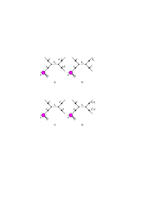
Figure 2: Lowest-order $s$-channel diagrams for first-generation squark production in $e^{+}p$ collisions at HERA. Diagrams a) and c) are the ${\not{R}_{p}}$ decays for $\tilde{{\bar{d}}}_{k}$ and $\tilde{u}_{j}$ squarks, respectively. The $R_{p}$-conserving decays are shown in b) and d). The decays of the charginos and neutralinos, $\chi^{0}_{i}$ and $\chi^{+}_{i}$, into SM particles depend on the parameters of the SUSY model and are not shown.

In SUSY, conservation of baryon and lepton number is expressed in terms of $R$-parity, $R_{p}$. It is defined as $R_{p}=(-1)^{3B+L+2S}$, where $B$ is the baryon number, $L$ is the lepton number and $S$ is the spin of the particle. Ordinary SM particles have $R_{p}=+1$ while their hypothetical supersymmetric partners have $R_{p}=-1$. In versions of the theory in which $R$-parity is not conserved, squarks (the SUSY counterparts to quarks) have the same production mechanism as a generic scalar resonance. The squark flavors listed in Table 3 have ${\not{R}_{p}}$ decays into lepton-jet final states. Figures 2a and c show the $s$-channel diagrams for these squark decays. The $\tilde{u}_{j}$ and the $\tilde{{\bar{d}}}_{k}$ squarks behave like $S_{e^{+}d}$ and $S_{e^{+}\bar{u}}$ resonant states, respectively (see Table 3), and the subscripts $j$ and $k$ denote the squark generation. Three generations are possible, but it is assumed that only a single generation has non-negligible coupling. These squarks would also be expected to have $R_{p}$-conserving decays into neutralinos ($\chi^{0}_{i}$) and charginos ($\chi^{+}_{i}$) (Figs. 2b and d) with multi-jet signatures different from $e^{+}$-jet and $\mkern 1.5mu\overline{\mkern-1.5mu\nu\mkern-1.0mu}\mkern 1.0mu$-jet. A detailed discussion of these states, whose properties depend on many SUSY parameters, is beyond the scope of this paper. The branching ratios of squarks into $e^{+}$-jet and $\mkern 1.5mu\overline{\mkern-1.5mu\nu\mkern-1.0mu}\mkern 1.0mu$-jet, as well as other final states, are therefore treated as free parameters in this paper.

4 Experimental conditions

During 1994-97, HERA collided protons of energy $E_{p}=820\,\mbox{GeV}$ with positrons of energy $E_{e}=27.5\,\mbox{GeV}$. The integrated luminosity of the data is $47.7\mbox{pb}^{-1}$. A detailed description of the ZEUS detector can be found elsewhere [15].  The primary components used in the present analysis are the central tracking detector (CTD) positioned in a 1.43 T solenoidal magnetic field, the uranium-scintillator sampling calorimeter (CAL) and the luminosity detector (LUMI).

The CTD [16] was used to establish an interaction vertex with a typical resolution of 3 cm in the beam direction for events considered in this analysis. Energy deposits in the CAL [17] were used to measure the positron energy and hadronic energy. The CAL has three sections: the forward, barrel, and rear calorimeters (FCAL, BCAL, and RCAL). The FCAL and BCAL are segmented longitudinally into an electromagnetic section (EMC) and two hadronic sections (HAC1, 2). The RCAL has one EMC and one HAC section. The cell structure is formed by scintillator tiles. The cells are arranged into towers consisting of $4$ EMC cells, a HAC1 cell and a HAC2 cell (in FCAL and BCAL). The transverse dimensions of the towers in FCAL are $20\times 20$ cm². One tower is absent at the center of the FCAL and RCAL to allow space for passage of the beams. Cells provide timing measurements with resolution better than 1 ns for energy deposits above 4.5 GeV. Signal times are useful for rejecting background from non-$ep$ sources and for determining the position of the interaction vertex if tracking information is unavailable.

Under test beam conditions, the CAL has a resolution of $0.18/\sqrt{E(\mbox{GeV})}$ for positrons hitting the center of a calorimeter cell, and $0.35/\sqrt{E(\mbox{GeV})}$ for single hadrons. The events of interest in this analysis have only hadronic jets, which impact primarily in the FCAL. In simulations, the jet energy resolution for the FCAL is found to average $\sigma/E=0.55/\sqrt{E(\mbox{GeV})}\oplus 0.02$ [3].

To reconstruct the hadronic system, corrections were applied for inactive material in front of the calorimeter. The overall hadronic energy scales of the FCAL and BCAL are determined to within $2\%$ by examining the $P_{T}$ balance of NC DIS events [18].

The luminosity was measured from the rate of the bremsstrahlung process $e^{+}p\rightarrow e^{+}p\gamma$ [19], and has an uncertainty of $1.6\%$.

A three-level trigger similar to the one used in the charged current analysis was used to select events online [4].

5 Event simulation

Standard Model CC events were simulated using the HERACLES 4.6.2 [20] program with the DJANGO 6 version 2.4 [21] interface to the hadronization programs. First- and second-generation quarks are simulated, while third-generation quarks were ignored [22] because of the large mass of the top quark and the small off-diagonal elements of the CKM matrix. The hadronic final state was simulated using the MEPS model in LEPTO 6.5 [23], which includes order-$\alpha_{S}$ matrix elements and models of higher-order QCD radiation. The color-dipole model in ARIADNE 4.08 [24] provided a systematic check. The CTEQ4D parton distribution set [11] with the Yang-Bodek correction, Eq. (8), was used to evaluate the nominal CC cross section, and the unmodified CTEQ4D PDF was used as an alternative PDF with smaller $d$-quark density.

Simulated resonant-state events were generated using PYTHIA 6.1 [25]. States with masses between 150 and 280 GeV were simulated in 10 GeV steps. This program takes into account the finite width of the resonant-state, but only includes the s-channel diagram. Initial- and final-state QCD radiation from the quark and the effect of LQ hadronization before decay are taken into account, as is initial-state QED radiation from the positron.

Generated events were input into a GEANT 3.13-based simulation [26] of the ZEUS detector.  Trigger and offline processing requirements as used for the data were applied to the simulated events.

6 Event selection

Events were selected with cuts similar to those used in the CC cross-section measurement from the same data [4]. The events were classified first according to $\gamma_{0}$, the hadronic scattering angle of the system relative to the nominal interaction point [4]. If $\gamma_{0}$ was sufficiently large, i.e. in the central region, tracks in the CTD were used to reconstruct the event vertex. On the other hand, if $\gamma_{0}$ was small, i.e. in the forward region, the hadronic final state of such $\mkern 1.5mu\overline{\mkern-1.5mu\nu\mkern-1.0mu}\mkern 1.0mu$-jet events was often outside the acceptance of the CTD, and thus the vertex position was obtained from the arrival time of particles entering the FCAL. The following selection cuts were then applied:

• to select high-mass $\mkern 1.5mu\overline{\mkern-1.5mu\nu\mkern-1.0mu}\mkern 1.0muX$ states, events were required to have substantial missing transverse momentum: ${\mbox{$\not{P}_{T}$}}>20$ GeV;

• a cut of $y<0.9$ discarded events in which the kinematic variables were poorly reconstructed;

• events with ${\mbox{$\not{P}_{T}$}}/E_{T}<0.4$ (where $E_{T}$ denotes the total transverse energy measured in the event) were removed to reject photoproduction background. For events with $\gamma_{0}<0.4$, this cut was increased to $0.6$;

• NC background was removed by discarding events with identified positrons;

• non-$ep$ collision events caused by beam-gas, halo muons, and cosmic rays were removed by a series of standard cuts based on the general topology expected for events from $ep$ collisions originating from the interaction region at the correct beam-crossing time.

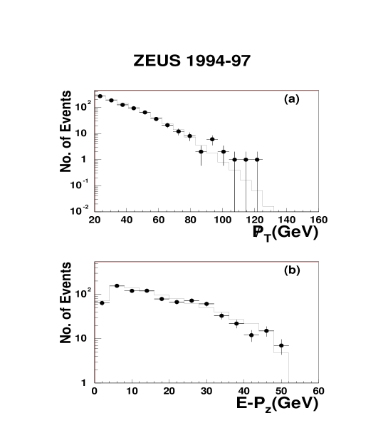
Figure 3: (a) The $\not{P}_{T}$ distribution for the final event sample. (b) The $(E-P_{Z})$ distribution. The points represent the data and the histogram is the SM MC prediction.

The final sample contains 829 events.

The momentum carried by the antineutrino is extracted from the $\not{P}_{T}$ and the longitudinal momentum variable $(E-P_{Z})$ of the event; distributions are shown in Fig. 3. The data and SM predictions agree except for ${\mbox{$\not{P}_{T}$}}>90$ GeV, where a slight excess is observed in the data. The $(E-P_{Z})$ distribution peaks near 10 GeV. These distributions are very different from those of NC events, which have small $\not{P}_{T}$ and an $(E-P_{Z})$ distribution peaked near twice the positron beam energy. These differences arise from the undetected final-state antineutrino in this sample.

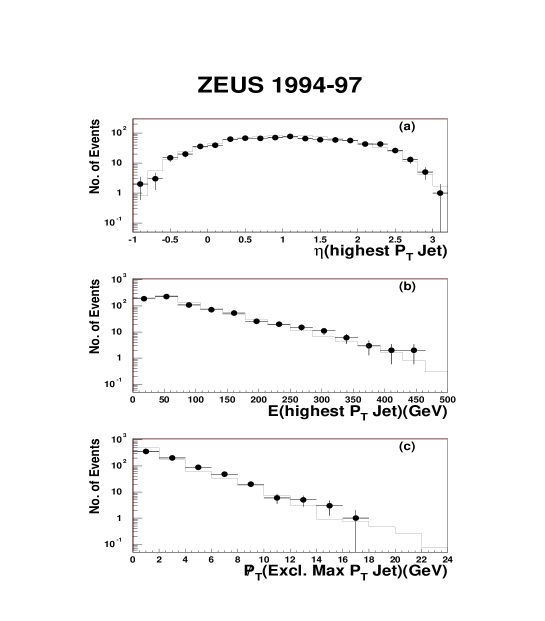
Figure 4: Comparison of jet distributions in the data and Monte Carlo. (a) The pseudorapidity, $\eta$, of the highest $P_{T}^{j}$ jet in each event. (b) The energy of the highest $P_{T}^{j}$ jet. (c) The missing transverse momentum $\not{P}_{T}$ in each event when the highest $P_{T}^{j}$ jet is excluded. The points represent the data and the histogram the SM Monte Carlo prediction.

Jets were identified using the longitudinally-invariant $k_{T}$-clustering algorithm [27] in inclusive mode [28]. At least one jet was required with transverse momentum $P_{T}^{j}>10\,\mbox{GeV}$. Fig. 4 shows the distributions of the pseudorapidity, $\eta$, of the highest $P_{T}^{j}$ jet . Also shown, for each event, are the energy of the highest $P_{T}^{j}$ jet and the $\not{P}_{T}$ when the momentum of the highest $P_{T}^{j}$ jet is excluded. Reasonable agreement is observed between the data and SM predictions in each case.

The outer boundary of the inner ring of FCAL towers was used to define a fiducial cut for the jet reconstruction. The centroid of the jet with the highest $P_{T}^{j}$ was required to be outside a $60\times 60$ cm² box on the face of the FCAL centered on the beam pipe. This restricts the pseudorapidity of the jet to be less than roughly $2.6$. This requirement removes 25 events, bringing the total sample to 804 events.

7 Mass and $\theta^{\ast}$ reconstruction

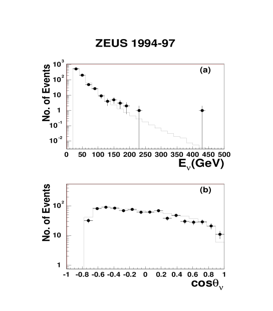
Figure 5: (a) The distribution of the energy of the final-state antineutrino in the lab frame, $E_{\nu}$. (b) The distribution of $\cos\theta_{\nu}$, where $\theta_{\nu}$ is the polar angle of the scattered antineutrino in the lab frame. The forward direction ($\cos\theta_{\nu}=1$) corresponds to the proton beam direction. The points are the data and the line is the SM Monte Carlo prediction.

It was assumed for the resonance search that all the missing momentum is carried away by one antineutrino. The invariant mass of the $\mkern 1.5mu\overline{\mkern-1.5mu\nu\mkern-1.0mu}\mkern 1.0mu$-jet system, $M_{\nu j}$, was calculated using Eq. (1) using only the highest $P_{T}^{j}$ jet. The jet direction was determined from the vector formed by the event vertex and the jet centroid in the calorimeter. The neutrino energy and angle were calculated as:

$$E_{\nu} = \frac{{\mbox{$\not{P}_{T}$}}^{2}+(E-P_{Z})_{\nu}^{2}}{2\cdot(E-P_{Z})_{\nu}}$$

$$\cos\theta_{\nu} = \frac{{\mbox{$\not{P}_{T}$}}^{2}-(E-P_{Z})_{\nu}^{2}}{{\mbox{$\not{P}_{T}$}}^{2}+(E-P_{Z})_{\nu}^{2}}$$

where $(E-P_{Z})_{\nu}=2E_{e}-(E-P_{Z})$. Distributions of the reconstructed antineutrino energy and polar angle in the laboratory frame ($E_{\nu}$ and $\cos\theta_{\nu}$) are shown in Fig. 5. Reasonable agreement is observed between data and the SM prediction. Monte Carlo simulations of resonant states indicate that the antineutrino energy and polar angle were measured with average resolutions of $16\%$ and $11\%$, respectively. The average systematic shift in $E_{\nu}$ was found to be less than $2\%$, while the shift in $\theta_{\nu}$ was less than $1\%$.

Monte Carlo simulations of resonant states were used to determine the resolution and estimate the possible bias for the reconstructed mass. The mass resolution was obtained by performing a Gaussian fit to the peak of the reconstructed mass spectrum. For resonant-state masses from 170 GeV to 270 GeV, the average mass resolution was found to be $7\%$. The peak position of the Gaussian differed from the generated mass by less than $2\%$ over the entire range.

Note that energy-momentum conservation, assumed in order to calculate $E_{\nu}$ and $\theta_{\nu}$, does not apply when undetected initial-state radiation (ISR) from the beam positron occurs. At high masses, QED radiation results in an underestimate of $E_{\nu}$ and an overestimate of $\theta_{\nu}$. This, as well as final-state QCD radiation, results in lower reconstructed masses, leading to an asymmetry in the expected mass distribution. In a simulation of a resonance of mass 220 GeV, only $1\%$ of events had an $M_{\nu j}$ more than $20\%$ higher than the true mass, while $16\%$ had an $M_{\nu j}$ more than $20\%$ lower than the true mass.

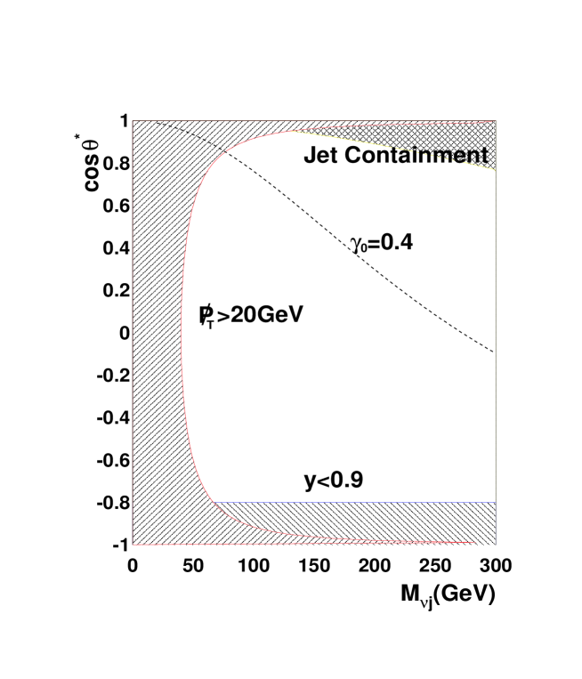
Figure 6: Acceptance in the $\cos\theta^{\ast}$-$M_{\nu j}$ plane. The shaded areas are the regions excluded by the requirements of ${\mbox{$\not{P}_{T}$}}>20$ GeV, $y<0.9$ and jet-containment assuming an $eq\rightarrow\mkern 1.5mu\overline{\mkern-1.5mu\nu\mkern-1.0mu}\mkern 1.0muq$ scattering at the nominal interaction point. No detector simulation is included. The dotted $\gamma_{0}=0.4$ line shows the boundary between events using the FCAL timing vertex (above) and the CTD tracking vertex (below).

In contrast to the resonance search, setting cross-section limits on $e^{+}p\rightarrow\bar{\nu}X$ processes requires that a specific production mechanism be assumed. For this reason, an invariant mass, $M_{\nu js}$, was calculated using all of the jets in the event with $P_{T}^{j}>10\,\mbox{GeV}$ and $\eta<3$. Monte Carlo studies show that, for narrow resonant states, using multiple jets gives more accurate mass reconstruction for events with more than one jet (for masses above 150 GeV, $12\%$ of the simulated LQ events have multiple jets).

The selection cuts described in Sect. 6 determine the kinematic region where mass reconstruction is possible. Figure 6 shows the approximate regions in the $\cos\theta^{\ast}$-$M_{\nu j}$ plane which are excluded by the requirements of ${\mbox{$\not{P}_{T}$}}>20$ GeV, $y<0.9$ and the jet containment for events originating from the nominal interaction point. In the unshaded regions, acceptance is typically $\approx 80\%$. The variable $\gamma$ denotes the scattering angle of the struck quark. Events above the $\gamma_{0}=0.4$ line typically use the FCAL timing vertex, while those below this line use the vertex found from CTD tracking.

8 Mass and $\cos\theta^{\ast}$ distributions

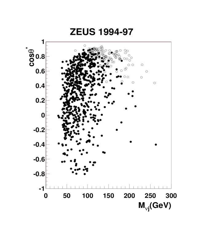
Figure 7: The distribution of the final event sample in the $M_{\nu j}$-$\cos\theta^{*}$ plane. Solid points indicate events reconstructed with a tracking vertex; open circles events reconstructed with a timing vertex.

Figure 7 shows the distribution of events in the $M_{\nu j}$ -$\cos\theta^{\ast}$ plane. The events populate the region of large acceptance described in Fig. 6.

8.1 Systematic uncertainties

The systematic uncertainties in the predicted rate of events range from about $7\%$ at $M_{\nu j}\approx 100\,\mbox{GeV}$ to about $20\%$ at $M_{\nu j}\approx 220\,\mbox{GeV}$, and over $40\%$ at $M_{\nu j}\approx 260\,\mbox{GeV}$.  The major sources of these are uncertainties in the calorimeter energy scale, uncertainties in the simulation of the hadronic energy flow (established by comparing results from the nominal LEPTO MEPS model with a Monte Carlo sample using the alternative ARIADNE model) and uncertainties in the parton distribution functions.

Potential sources of systematic error which were found to have negligible effects include reasonable variations of the selection cuts, background-contamination uncertainties, timing-vertex uncertainties, and the uncertainty in the luminosity determination.

8.2 Comparison with Standard Model

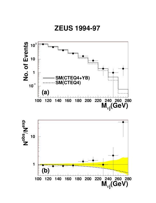
Figure 8: (a) The mass distribution for the data (points) and Monte Carlo (histograms). The dashed line shows the predicted mass spectrum when the CTEQ4D PDFs are used, while the solid curve shows the distribution predicted when the $d$-quark density is enhanced using the Yang-Bodek correction (see Eq. (8)). (b) The ratio of the number of events observed to the number expected, $N^{obs}/N^{exp}$, obtained using the Yang-Bodek correction. The shaded band indicates the systematic error in the SM expectation. The dashed line shows the SM expectation when the Yang-Bodek correction is not implemented. The error bars on the data points are calculated from the square root of the number of events in the bin.

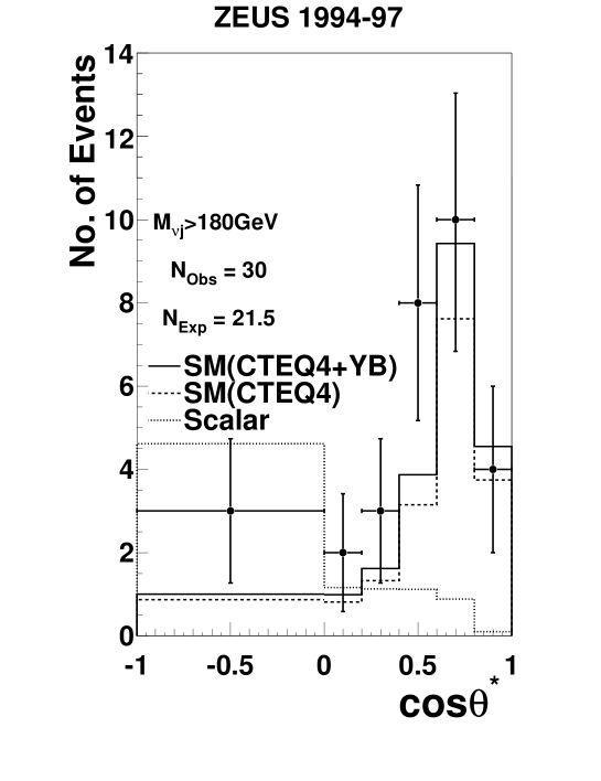
Figure 9: The $\cos\theta^{*}$ distribution of events with $M_{\nu j}>180\;\mbox{GeV}$. The dashed line shows the predicted $\cos\theta^{\ast}$ spectrum when the CTEQ4D PDFs are used, while the solid curve shows the distribution predicted when the $d$-quark density is enhanced using the Yang-Bodek correction (Eq. (8)). Also shown is the $\cos\theta^{\ast}$ distribution for a scalar resonance (dotted line) normalized to 9 events.

In Fig. 8(a), the observed mass distribution is compared to the SM predictions from Monte Carlo simulations using the CTEQ4D parton densities [11] and the CTEQ4D PDF modified by the Yang-Bodek correction of Eq. (8). The predictions using the CTEQ5 [9] or the NLO QCD fit by Botje [6] are similar to the modified CTEQ4D predictions. For $M_{\nu j}>180\;\mbox{GeV}$, the data tend to lie above the expectations. There are 30 events observed in this region, while $21.5\pm 3.3$ are predicted ($16.0\pm 2.4$ events for CTEQ4D without the correction of Eq. (8)). The uncertainty on the predicted number of events is due to the effects described above.

Figure 9 shows the $\cos\theta^{\ast}$ distribution of the events with $M_{\nu j}>180\;\mbox{GeV}$ together with the distribution expected for decay of a narrow scalar resonance (normalized to 9 events). In the $\cos\theta^{\ast}<0.4$ region where the DIS background is suppressed, 8 data events are observed while $3.6\pm 0.5$ SM events are expected.

Given the limited statistics in the present data and the systematic uncertainties of the SM predictions, the observed mass spectrum is compatible with SM expectations.

9 Limits on resonant-state production

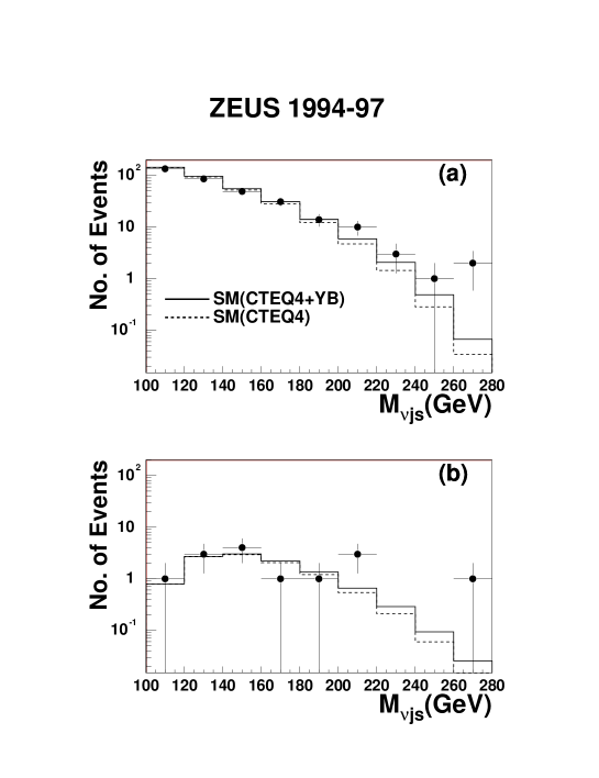
Figure 10: a) The reconstructed mass spectrum using multiple jets for data (points) and SM expectation (histogram). b) The mass spectrum using multiple jets after the cut ($\cos\theta^{\ast}<\cos\theta_{{\rm max}}^{\ast}$) for the scalar resonance search has been applied.

Since there is no evidence for a narrow resonance in the $\mkern 1.5mu\overline{\mkern-1.5mu\nu\mkern-1.0mu}\mkern 1.0mu$-jet data, limits may be set on the production of the resonant states listed in Table 1. Since such states would need to have a positron as well as an antineutrino decay channel, the cross-section limits were set using these $\mkern 1.5mu\overline{\mkern-1.5mu\nu\mkern-1.0mu}\mkern 1.0mu$-jet data along with the $e^{+}$-jet data previously reported [3]. Only couplings $\lambda\leq 1$ are considered. The limit-setting procedure assumes the states have the same production and decay mechanism as the Monte Carlo used to generate the resonance events. The invariant mass reconstructed using the neutrino and all jets with ${\mbox{$\not{P}_{T}$}}>10$ GeV and $\eta<3.0$, $M_{\nu js}$, was used to set limits. The mass spectrum reconstructed with this technique is shown in Fig. 10a, and is similar to that from single jets (Fig. 8).

The limit-setting procedure requires two parameters at each value of $M_{\nu js}$: the mass window, $\Delta M_{\nu js}$, and an upper cut ($\cos\theta_{{\rm max}}^{\ast}$) on the measured value of $\cos\theta^{\ast}$.  Simulations of both SM background and resonant signals were used to find values for these parameters which optimize observation of a signal relative to DIS background.  For a scalar resonance with a $\mkern 1.5mu\overline{\mkern-1.5mu\nu\mkern-1.0mu}\mkern 1.0mu$-jet final state, $\Delta M_{\nu js}$ ranged from 20 to 35 GeV in the 160-280 GeV mass range, while in the same range $\cos\theta_{{\rm max}}^{\ast}$ increased from 0.2 to 0.8. For a vector resonance in the same $M_{\nu js}$ range, $\Delta M_{\nu js}$ increased from 15 to 35 GeV, while $\cos\theta_{{\rm max}}^{\ast}$ increased from 0.6 to 0.84. The mass spectrum after applying the optimal $\cos\theta^{\ast}$ cut for the scalar search is shown in Fig. 10b. A similar optimization procedure, performed for the $e^{+}$-jet final state using the NC data, has been described in a previous publication [3].

To find the $95\%$ confidence level (CL) upper limit on the resonant-state cross section, $\sigma_{\rm lim}$, a likelihood is calculated using the Poisson probability for each decay channel:

$$L_{c}(\sigma)=e^{-(\mathcal{L}\beta_{c}\epsilon_{c}\sigma+N_{c}^{\rm bkg})}\frac{(\mathcal{L}\beta_{c}\epsilon_{c}\sigma+N_{c}^{\rm bkg})^{N_{c}^{\rm obs}}}{N_{c}^{\rm obs}!},$$ (12)

where $\mathcal{L}$ is the luminosity, $\beta_{c}$ is the branching ratio of the decay channel, $N_{c}^{\rm obs}$ is the number of observed events, $N_{c}^{\rm bkg}$ is the expected number of DIS background, and $\epsilon_{c}$ is the acceptance calculated from resonance Monte Carlo. The subscript $c$ denotes the decay channel, which for this analysis is either $\bar{\nu}q$ or $e^{+}q$, for the CC-like and NC-like final states, respectively. If more than one channel was used to set a limit, the likelihoods for each channel were multiplied together to get the total likelihood, $L(\sigma)$. A flat prior probability density for the cross section $\sigma$ was assumed, such that the probability density, $f(\sigma)$, is simply $f(\sigma)\propto L(\sigma)$. A limit was then obtained on the cross section, $\sigma_{\rm lim}$, by solving:

$$\int_{0}^{\sigma_{\rm lim}}d\sigma f(\sigma)=0.95\int_{0}^{\infty}d\sigma f(\sigma)$$ (13)

and the resulting cross-section limit was converted to a coupling limit $\lambda_{\rm lim}$ using the NWA (Eq. (11)). Note that using two channels does not always produce a stronger limit than using a single channel.

The limits on $\lambda$ depend on the accuracy of the NWA. Comparisons between the NWA and the full resonant-state cross sections show that the NWA was too high by up to a factor $1.7$ for $S_{e^{+}\bar{u}}$. This was corrected for in setting the limits. For all other states, the NWA provides a reasonable approximation of the full resonant-state cross section in the mass and coupling ranges studied.

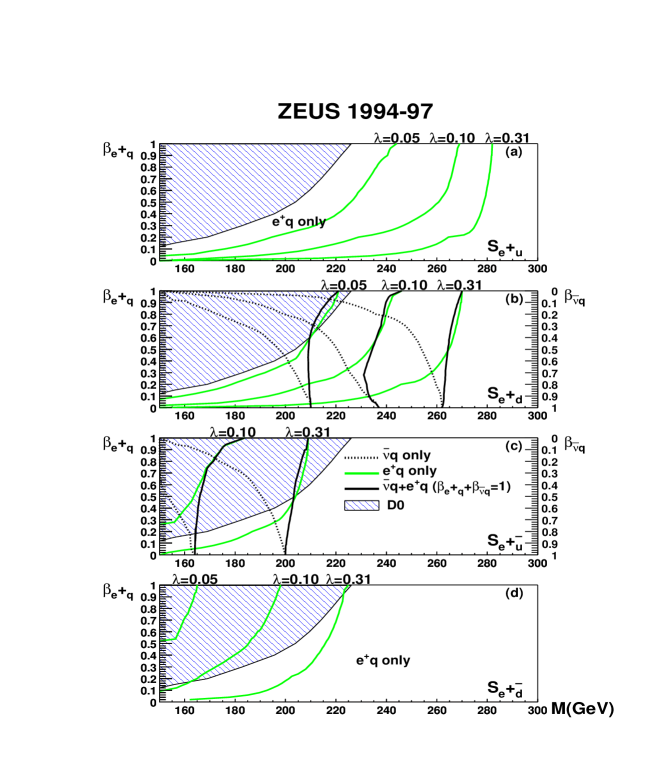
Figure 11: The branching ratios into $e^{+}q$ and $\mkern 1.5mu\overline{\mkern-1.5mu\nu\mkern-1.0mu}\mkern 1.0muq$ (shown on the left and right axes, respectively) vs. excluded mass for the scalar resonant states listed in Table 1. For each limit curve, the area to the left of the curve is the excluded region. Results for $e^{+}\mkern 1.5mu\overline{\mkern-1.5muu\mkern-1.0mu}\mkern 1.0mu$, $e^{+}\mkern 1.5mu\overline{\mkern-1.5mud\mkern-1.0mu}\mkern 1.0mu$, $e^{+}u$ and $e^{+}d$ resonant states are shown for coupling strengths of $\lambda=0.05$, $\lambda=0.10$, and $\lambda=0.31$. The shaded region in each plot shows the mass range excluded by the D0 experiment. For (a) $e^{+}u$ and (d) $e^{+}\mkern 1.5mu\overline{\mkern-1.5mud\mkern-1.0mu}\mkern 1.0mu$ resonant states, limits were set using only $e^{+}q$ data since $\mkern 1.5mu\overline{\mkern-1.5mu\nu\mkern-1.0mu}\mkern 1.0muq$ decays are forbidden by charge conservation. The (b) $e^{+}d$ and (c) $e^{+}\mkern 1.5mu\overline{\mkern-1.5muu\mkern-1.0mu}\mkern 1.0mu$ states have both $e^{+}q$ and $\mkern 1.5mu\overline{\mkern-1.5mu\nu\mkern-1.0mu}\mkern 1.0muq$ decay channels. The dotted line corresponds to only $\mkern 1.5mu\overline{\mkern-1.5mu\nu\mkern-1.0mu}\mkern 1.0muq$ data, the shaded line corresponds to only $e^{+}q$ data, and the solid black line corresponds to both the $e^{+}q$ and the $\mkern 1.5mu\overline{\mkern-1.5mu\nu\mkern-1.0mu}\mkern 1.0muq$ data sets. The combined limits were calculated assuming that $\beta_{\mkern 1.5mu\overline{\mkern-1.5mu\nu\mkern-1.0mu}\mkern 1.0muq}+\beta_{e^{+}q}=1$.

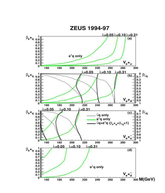
Figure 12: The branching ratios into $e^{+}q$ and $\mkern 1.5mu\overline{\mkern-1.5mu\nu\mkern-1.0mu}\mkern 1.0muq$ (shown on the left and right axes, respectively) vs. excluded mass for the vector resonant states listed in Table 1. For each limit curve, the area to the left of the curve is the excluded region. Results for $e^{+}\mkern 1.5mu\overline{\mkern-1.5muu\mkern-1.0mu}\mkern 1.0mu$, $e^{+}\mkern 1.5mu\overline{\mkern-1.5mud\mkern-1.0mu}\mkern 1.0mu$, $e^{+}u$ and $e^{+}d$ resonant states are shown for coupling strengths of $\lambda=0.05$, $\lambda=0.10$, and $\lambda=0.31$. For (a) $e^{+}u$ and (d) $e^{+}\mkern 1.5mu\overline{\mkern-1.5mud\mkern-1.0mu}\mkern 1.0mu$ resonant states, limits were set using only $e^{+}q$ data since $\mkern 1.5mu\overline{\mkern-1.5mu\nu\mkern-1.0mu}\mkern 1.0muq$ decays are forbidden by charge conservation. The (b) $e^{+}d$ and (c) $e^{+}\mkern 1.5mu\overline{\mkern-1.5muu\mkern-1.0mu}\mkern 1.0mu$ states have both $e^{+}q$ and $\mkern 1.5mu\overline{\mkern-1.5mu\nu\mkern-1.0mu}\mkern 1.0muq$ decay channels. The dotted line corresponds to only $\mkern 1.5mu\overline{\mkern-1.5mu\nu\mkern-1.0mu}\mkern 1.0muq$ data, the shaded line corresponds to only $e^{+}q$ data, and the solid black line corresponds to both the $e^{+}q$ and the $\mkern 1.5mu\overline{\mkern-1.5mu\nu\mkern-1.0mu}\mkern 1.0muq$ data sets. The combined limits were calculated assuming that $\beta_{\mkern 1.5mu\overline{\mkern-1.5mu\nu\mkern-1.0mu}\mkern 1.0muq}+\beta_{e^{+}q}=1$.

Figure 11 shows the limits obtained for the four scalar resonant states of Table 1 as a function of $\beta_{e^{+}q}$ and $\beta_{\mkern 1.5mu\overline{\mkern-1.5mu\nu\mkern-1.0mu}\mkern 1.0muq}$, the branching ratios into $e^{+}q$ and $\mkern 1.5mu\overline{\mkern-1.5mu\nu\mkern-1.0mu}\mkern 1.0muq$, respectively. The equivalent plots for vector resonant states are shown in Fig. 12. The limits were calculated for coupling strengths of $\lambda=0.05$ and $\lambda=0.10$, as well as for coupling $\lambda=0.31\approx\sqrt{4\pi\alpha}$. For the $e^{+}u$ and $e^{+}\bar{d}$ resonances (a and d in Figs. 11 and 12), $\mkern 1.5mu\overline{\mkern-1.5mu\nu\mkern-1.0mu}\mkern 1.0muq$ decays are forbidden by charge conservation, so the limits are set using only the $e^{+}q$ channel. The $e^{+}\bar{u}$ and $e^{+}d$ resonances (b and c) can provide both $e^{+}q$ and $\mkern 1.5mu\overline{\mkern-1.5mu\nu\mkern-1.0mu}\mkern 1.0muq$ decays, so limits are calculated using the $e^{+}$-jet and $\mkern 1.5mu\overline{\mkern-1.5mu\nu\mkern-1.0mu}\mkern 1.0mu$-jet data sets separately and combined. The combined $e^{+}q\!+\!\mkern 1.5mu\overline{\mkern-1.5mu\nu\mkern-1.0mu}\mkern 1.0muq$ limits, which assume $\beta_{\mkern 1.5mu\overline{\mkern-1.5mu\nu\mkern-1.0mu}\mkern 1.0muq}+\beta_{e^{+}q}=1$, are largely independent of branching ratio. The limits obtained using only the $e^{+}$-jet (or the $\mkern 1.5mu\overline{\mkern-1.5mu\nu\mkern-1.0mu}\mkern 1.0mu$-jet) data allow for decay modes other than $e^{+}q$ and $\mkern 1.5mu\overline{\mkern-1.5mu\nu\mkern-1.0mu}\mkern 1.0muq$, so the $e^{+}q$ and the $\mkern 1.5mu\overline{\mkern-1.5mu\nu\mkern-1.0mu}\mkern 1.0muq$ limits are applicable to a wider range of physics models than the combined $e^{+}q\!+\!\mkern 1.5mu\overline{\mkern-1.5mu\nu\mkern-1.0mu}\mkern 1.0muq$ results. The systematic uncertainties on the predicted background described in Section 8.1 were found to change the excluded mass limits by less than $1\%$ for $M_{\nu j}>220$ GeV, and have therefore been neglected.

The $e^{+}q$ and $\mkern 1.5mu\overline{\mkern-1.5mu\nu\mkern-1.0mu}\mkern 1.0muq$ data have also been used to set limits on scalar and vector resonances with second generation quarks. Assuming a coupling strength of $\lambda=0.31$ the mass limits for $e^{+}s$ states decaying with 50 % branching ratio to $e^{+}q$ and with 50 % to $\mkern 1.5mu\overline{\mkern-1.5mu\nu\mkern-1.0mu}\mkern 1.0muq$ are 207 GeV for a scalar and 211 GeV for a vector state.

For comparison, the limits on scalar resonances obtained by the D0 experiment [29] at the Tevatron are shown by the shaded region. These limits are independent of both coupling and quark flavor. Similar results to those presented here have been published by the H1 experiment [30].

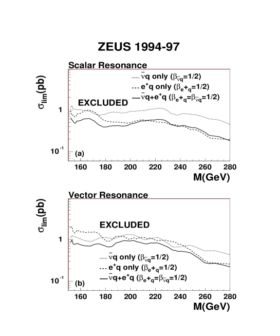
Figure 13: (a) Limits on the total production cross section for a narrow scalar resonant state. (b) The corresponding limits for a narrow vector resonant state. Limits derived from $e^{+}q$ ($\mkern 1.5mu\overline{\mkern-1.5mu\nu\mkern-1.0mu}\mkern 1.0muq$) assume a branching ratio $\beta_{e^{+}q}$ ($\beta_{\mkern 1.5mu\overline{\mkern-1.5mu\nu\mkern-1.0mu}\mkern 1.0muq}$) of 1/2, while the combined $e^{+}q\!+\!\mkern 1.5mu\overline{\mkern-1.5mu\nu\mkern-1.0mu}\mkern 1.0muq$ limits assume branching ratios of $\beta_{e^{+}q}=\beta_{\mkern 1.5mu\overline{\mkern-1.5mu\nu\mkern-1.0mu}\mkern 1.0muq}=1/2$.

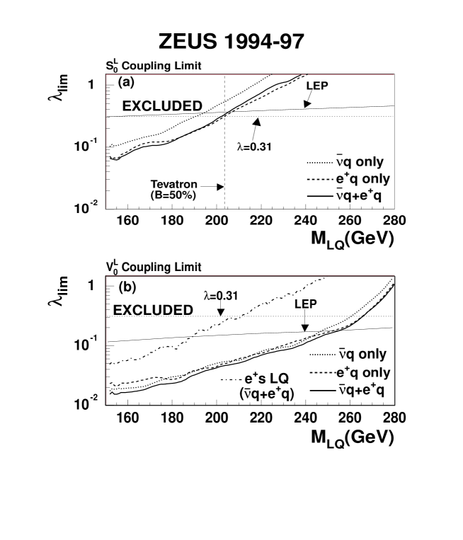
Figure 14: (a) The limits on the coupling $\lambda_{\rm lim}$ for an $S_{0}^{L}$ LQ. (b) The same for a $V_{0}^{L}$ LQ. Results from the $\mkern 1.5mu\overline{\mkern-1.5mu\nu\mkern-1.0mu}\mkern 1.0muq$ and $e^{+}q$ channels are shown, along with the limits obtained by combining the two channels. Also shown is the limit for second generation LQ’s (dashed-dotted line). In both plots, the horizontal line indicates the coupling $\lambda=0.31\approx\sqrt{4\pi\alpha}$. For comparison, representative limits from the Tevatron [29] and LEP [31] are also shown.

10 Model-dependent limits

The limits on generic resonant states were converted to limits on the production of LQ and squarks that have $e^{+}q$ and $\mkern 1.5mu\overline{\mkern-1.5mu\nu\mkern-1.0mu}\mkern 1.0muq$ decays. Figure 13 shows the limit on the production cross section, $\sigma_{\rm lim}$, for scalar and vector resonant states. Limits derived from $e^{+}q$ ($\mkern 1.5mu\overline{\mkern-1.5mu\nu\mkern-1.0mu}\mkern 1.0muq$) assume a branching ratio $\beta_{e^{+}q}$ ($\beta_{\mkern 1.5mu\overline{\mkern-1.5mu\nu\mkern-1.0mu}\mkern 1.0muq}$) of 1/2, while the combined $e^{+}q\!+\!\mkern 1.5mu\overline{\mkern-1.5mu\nu\mkern-1.0mu}\mkern 1.0muq$ limits assume branching ratios of $\beta_{e^{+}q}=\beta_{\mkern 1.5mu\overline{\mkern-1.5mu\nu\mkern-1.0mu}\mkern 1.0muq}=1/2$.

10.1 Leptoquarks limits

The cross-section limits were converted to limits on leptoquark coupling using Eq. (11). Figure 14 shows the coupling limits for the $S_{0}^{L}$ and $V_{0}^{L}$ LQ species listed in Table 2. If a coupling strength $\lambda=0.31\approx\sqrt{4\pi\alpha}$ is assumed, the production of an $S_{0}^{L}$ LQ is excluded up to a mass of 204 GeV with $95$ % CL, while the production of a $V_{0}^{L}$ LQ is excluded up to a mass of 265 GeV. When the $\mkern 1.5mu\overline{\mkern-1.5mu\nu\mkern-1.0mu}\mkern 1.0muq$ and $e^{+}q$ limits are combined, the resulting limits exclude approximately the same mass range as the $e^{+}q$-only limit. Also shown in Fig. 14 is the limit curve for second generation LQ’s of the type $V^{0}_{L}$ produced as an $e^{+}s$ resonance. The combined limits from $e^{+}q$ and $\mkern 1.5mu\overline{\mkern-1.5mu\nu\mkern-1.0mu}\mkern 1.0muq$ decays are shown. For comparison, limits from the D0 experiment with a branching ratio of $\beta_{e^{+}q}=1/2$ are shown [29]. Also included are LQ limits from the OPAL experiment at LEP [31].

10.2 SUSY limits

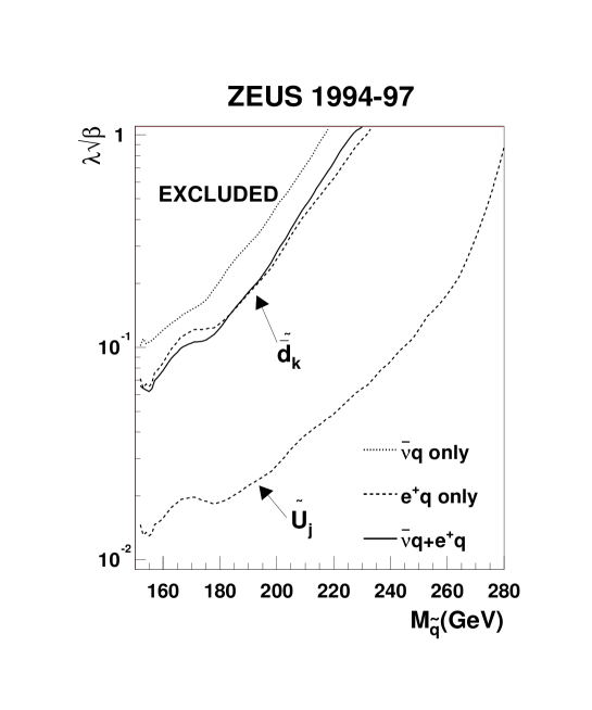
Figure 15: The limits on the coupling $\lambda\sqrt{\beta}$, where $\beta=\beta_{e^{+}q}+\beta_{\mkern 1.5mu\overline{\mkern-1.5mu\nu\mkern-1.0mu}\mkern 1.0muq}$. For the $\tilde{\bar{d}}_{k}$ squark, $\beta_{e^{+}q}=\beta_{\mkern 1.5mu\overline{\mkern-1.5mu\nu\mkern-1.0mu}\mkern 1.0muq}$, so results from the $\mkern 1.5mu\overline{\mkern-1.5mu\nu\mkern-1.0mu}\mkern 1.0mu$-jet and $e^{+}$-jet channels are shown, along with the limit obtained by combining the two channels. The $\tilde{u}_{j}$ limits are calculated using only $e^{+}q$ data since the gauge invariance of the SUSY superpotential requires $\beta_{\mkern 1.5mu\overline{\mkern-1.5mu\nu\mkern-1.0mu}\mkern 1.0muq}=0$.

Limits were set on the production of the squarks listed in Table 3. In addition to ${\not{R}_{p}}$ decays into $e^{+}q$ and $\mkern 1.5mu\overline{\mkern-1.5mu\nu\mkern-1.0mu}\mkern 1.0muq$, squarks can also have $R_{p}$-conserving decays into other final states. To remove the dependence on the branching ratios into these ${R}_{p}$-conserving states, limits were set on the quantity $\lambda\sqrt{\beta}$, where $\beta=\beta_{e^{+}q}+\beta_{\mkern 1.5mu\overline{\mkern-1.5mu\nu\mkern-1.0mu}\mkern 1.0muq}$. The limit-setting procedure does not account for possible contributions to the $e^{+}$-jet and $\mkern 1.5mu\overline{\mkern-1.5mu\nu\mkern-1.0mu}\mkern 1.0mu$-jet channels from $R_{p}$-conserving decays. Limits on $\tilde{{\bar{d}}}_{k}$ and $\tilde{u}_{j}$ are shown in Fig. 15. Because $\beta_{e^{+}q}=\beta_{\mkern 1.5mu\overline{\mkern-1.5mu\nu\mkern-1.0mu}\mkern 1.0muq}$ for the $\tilde{{\bar{d}}}_{k}$ decays, the combined $e^{+}q\!+\!\mkern 1.5mu\overline{\mkern-1.5mu\nu\mkern-1.0mu}\mkern 1.0muq$ limits are shown along with the limits obtained from the individual decay channels. For the $\tilde{u}_{j}$ squark, $\beta=\beta_{e^{+}q}$ since $\mkern 1.5mu\overline{\mkern-1.5mu\nu\mkern-1.0mu}\mkern 1.0muq$ decays would violate gauge invariance. Previous limits on ${\not{R}_{p}}$-squark production from smaller data sets have been set by the H1 experiment [32].

11 Conclusion

A study of the $\bar{\nu}$-jet mass spectrum in $e^{+}p\rightarrow\bar{\nu}X$ events at center-of-mass energy 300 GeV has been performed with the ZEUS detector at HERA using an integrated luminosity of $47.7\mbox{pb}^{-1}$. Events with topologies similar to high-$Q^{2}$ charged current DIS were selected. The invariant mass, $M_{\nu j}$, was calculated from the jet with the highest transverse energy and the antineutrino four-momenta.  The jet momentum was measured directly, while the antineutrino momentum was deduced from the energy-momentum imbalance measured in the detector. No evidence for a narrow resonance was observed. This analysis complements an earlier search for narrow resonances in the $e^{+}$-jet final state.

In the absence of evidence for a high-mass resonant state, the $e^{+}$-jet and $\mkern 1.5mu\overline{\mkern-1.5mu\nu\mkern-1.0mu}\mkern 1.0mu$-jet data sets were used to set limits on the production cross section of scalar and vector states decaying by either mode. Sensitivity to a resonant signal was optimized by restricting the center-of-mass decay angle to remove most DIS background and by choosing an appropriate mass window. The resulting cross-section limits were converted to coupling limits on $e^{+}u$, $e^{+}d$, $e^{+}\bar{u}$ and $e^{+}\bar{d}$ resonant states.

First-generation couplings between initial- and final-state quarks and leptons which conserve flavor and electric charge were considered. Limits were calculated as a function of the $e^{+}q$ and $\mkern 1.5mu\overline{\mkern-1.5mu\nu\mkern-1.0mu}\mkern 1.0muq$ branching ratios for small couplings and do not depend on a specific production mechanism. For resonances with both $e^{+}q$ and $\mkern 1.5mu\overline{\mkern-1.5mu\nu\mkern-1.0mu}\mkern 1.0muq$ decays, using both the $e^{+}$-jet and $\mkern 1.5mu\overline{\mkern-1.5mu\nu\mkern-1.0mu}\mkern 1.0mu$-jet data gave limits which are largely independent of the branching ratio if the state is assumed to have no additional decay modes.

The limits on generic resonant states were used to constrain the production of leptoquarks and $R_{p}$-violating squarks. For leptoquark flavors whose branching ratios into $e^{+}q$ and $\mkern 1.5mu\overline{\mkern-1.5mu\nu\mkern-1.0mu}\mkern 1.0muq$ are the same, exclusion limits of 204 GeV for scalars and 265 GeV for vectors were obtained if a coupling strength $\lambda=0.31$ is assumed. Limits on the production of $\tilde{{u}}_{j}$ and $\tilde{{\bar{d}}}_{k}$ squarks were obtained directly from the limits on $e^{+}d$ and $e^{+}\bar{u}$ resonances, respectively.

References

- [1] W. Buchmüller, R. Rückl and D. Wyler, Phys. Lett. B191 442 (1987); erratum Phys. Lett. B448 320 (1999).
- [2] J. Butterworth and H. Dreiner, Nucl. Phys. B397 3 (1993), and references therein.
- [3] ZEUS Collaboration, J. Breitweg et al., Eur. Phys. J. C16 253 (2000).
- [4] ZEUS Collaboration, J. Breitweg et al. Eur. Phys. J. C12 411 (2000).
- [5] G. Ingelman and R. Rückl, Phys. Lett. B201 369 (1988).
- [6] M. Botje, Eur. Phys. J. C14 285 (2000).
-
[7]
W. Melnitchouk and A.W. Thomas,
Phys. Lett. B377 11 (1996);
W. Melnitchouk and J.C. Peng, Phys. Lett. B400 220 (1997). - [8] U.K. Yang and A. Bodek, Phys. Rev. Lett. 82 2467 (1999).
- [9] CTEQ Collaboration, H.L. Lai et al., Eur. Phys. J. C12 375 (2000).
- [10] A.D. Martin, R.G. Roberts and W.J. Stirling, Phys. Lett. B387 419 (1996).
- [11] CTEQ Collaboration, H.L. Lai et al., Phys. Rev. D55 1280 (1997).
- [12] A.D. Martin, R.G. Roberts, W.J. Stirling and R.S Thorne, Eur. Phys. J. C4 463 (1998).
-
[13]
T. Plehn et al., Z. Phys. C74 611 (1997);
Z. Kunszt and W. J. Stirling, Z. Phys. C75 453 (1997). - [14] J. Blümlein, E. Boos and A. Kryukov, Z. Phys. C76 137 (1997).
- [15] ZEUS Collaboration, ‘The ZEUS Detector, Status Report 1993’, DESY (1993).
-
[16]
N. Harnew et al., Nucl. Inst. Methods A279 290 (1989);
B. Foster et al., Nucl. Phys. B (Proc. Suppl.) 32 181 (1993);
B. Foster et al., Nucl. Inst. Methods A 338 254 (1994). -
[17]
M. Derrick et al., Nucl. Inst. Methods A309 77 (1991);
A. Andresen et al., Nucl. Inst. Methods A309 101 (1991);
A. Caldwell et al., Nucl. Inst. Methods A321 356 (1992);
A. Bernstein et al., Nucl. Inst. Methods A336 23 (1993). - [18] ZEUS Collaboration, J. Breitweg et al., Eur. Phys. J. C11 427 (1999).
-
[19]
J. Andruszków et al., DESY 92-066 (1992);
ZEUS Collab., M. Derrick et al., Z. Phys. C 63 391 (1994). - [20] A. Kwiatkowski, H. Spiesberger and H.-J. Möring, Comp. Phys. Commun. 69 155 (1992).
- [21] K. Charchula, G. A. Schuler and H. Spiesberger, Comp. Phys. Commun. 81 381 (1994).
- [22] U.F. Katz, Deep Inelastic Positron–Proton Scattering in the High-Momentum-Transfer Regime of HERA, Springer Tracts in Modern Physics, Vol. 168, (2000).
- [23] G. Ingelman, A. Edin and J. Rathsman, Comp. Phys. Commun. 101 108 (1997).
- [24] L. Lönnblad, Comp. Phys. Commun. 71 15 (1992).
- [25] C. Friberg, E. Norrbin and T. Sjöstrand, Phys. Lett. B403 329 (1997).
- [26] R. Brun et al., CERN-DD/EE/84-1 (1987).
- [27] S. Catani et al., Nucl. Phys. B406 187 (1993).
- [28] S.D. Ellis and D.E. Soper, Phys. Rev. D48 3160 (1993).
- [29] D0 Collaboration, B. Abbott et al., Phys. Rev. Lett. 80 2051 (1998).
- [30] H1 Collaboration, C. Adloff et al., Eur. Phys. J. C11 447 (1999) and Erratum Eur. Phys. J C14 553 (2000).
- [31] OPAL Collaboration, G. Abbiendi et al., Eur. Phys. J. C6 1 (1999).
- [32] H1 Collaboration, S. Aid et al., Z. Phys. C71 211 (1996).