Abstract

The decay $\rm B^{0}\rightarrow J/\psi\,K^{0}_{S}$ is reconstructed with $\rm J/\psi\rightarrow e^{+}e^{-}$ or $\mu^{+}\mu^{-}$ and $\rm K^{0}_{S}\rightarrow\pi^{+}\pi^{-}$. From the full ALEPH dataset at LEP1 of about 4 million hadronic Z decays, 23 candidates are selected with an estimated purity of 71%. They are used to measure the CP asymmetry of this decay, given by $\sin 2\beta$ in the Standard Model, with the result $\sin 2\beta=0.84\ ^{+0.82}_{-1.04}\pm 0.16$. This is combined with existing measurements from other experiments, and increases the confidence level that CP violation has been observed in this channel to 98%.

Submitted to Physics Letters

The ALEPH Collaboration

R. Barate, D. Decamp, P. Ghez, C. Goy, J.-P. Lees, E. Merle, M.-N. Minard, B. Pietrzyk

Laboratoire de Physique des Particules (LAPP), IN²P³-CNRS, F-74019 Annecy-le-Vieux Cedex, France

S. Bravo, M.P. Casado, M. Chmeissani, J.M. Crespo, E. Fernandez, M. Fernandez-Bosman, Ll. Garrido,¹⁵ E. Graugés, M. Martinez, G. Merino, R. Miquel, Ll.M. Mir, A. Pacheco, H. Ruiz

Institut de Física d’Altes Energies, Universitat Autònoma de Barcelona, E-08193 Bellaterra (Barcelona), Spain⁷

A. Colaleo, D. Creanza, M. de Palma, G. Iaselli, G. Maggi, M. Maggi,¹ S. Nuzzo, A. Ranieri, G. Raso,²³ F. Ruggieri, G. Selvaggi, L. Silvestris, P. Tempesta, A. Tricomi,³ G. Zito

Dipartimento di Fisica, INFN Sezione di Bari, I-70126 Bari, Italy

X. Huang, J. Lin, Q. Ouyang, T. Wang, Y. Xie, R. Xu, S. Xue, J. Zhang, L. Zhang, W. Zhao

Institute of High Energy Physics, Academia Sinica, Beijing, The People’s Republic of China⁸

D. Abbaneo, G. Boix,⁶ O. Buchmüller, M. Cattaneo, F. Cerutti, G. Dissertori, H. Drevermann, R.W. Forty, M. Frank, T.C. Greening, J.B. Hansen, J. Harvey, P. Janot, B. Jost, I. Lehraus, P. Mato, A. Minten, A. Moutoussi, F. Ranjard, L. Rolandi, D. Schlatter, M. Schmitt,²⁰ O. Schneider,² P. Spagnolo, W. Tejessy, F. Teubert, E. Tournefier, A.E. Wright

European Laboratory for Particle Physics (CERN), CH-1211 Geneva 23, Switzerland

Z. Ajaltouni, F. Badaud, G. Chazelle, O. Deschamps, A. Falvard, P. Gay, C. Guicheney, P. Henrard, J. Jousset, B. Michel, S. Monteil, J-C. Montret, D. Pallin, P. Perret, F. Podlyski

Laboratoire de Physique Corpusculaire, Université Blaise Pascal, IN²P³-CNRS, Clermont-Ferrand, F-63177 Aubière, France

J.D. Hansen, J.R. Hansen, P.H. Hansen, B.S. Nilsson, B.A. Petersen, A. Wäänänen

Niels Bohr Institute, DK-2100 Copenhagen, Denmark⁹

G. Daskalakis, A. Kyriakis, C. Markou, E. Simopoulou, A. Vayaki

Nuclear Research Center Demokritos (NRCD), GR-15310 Attiki, Greece

A. Blondel,¹² G. Bonneaud, J.-C. Brient, A. Rougé, M. Rumpf, M. Swynghedauw, M. Verderi, H. Videau

Laboratoire de Physique Nucléaire et des Hautes Energies, Ecole Polytechnique, IN²P³-CNRS, F-91128 Palaiseau Cedex, France

E. Focardi, G. Parrini, K. Zachariadou

Dipartimento di Fisica, Università di Firenze, INFN Sezione di Firenze, I-50125 Firenze, Italy

A. Antonelli, M. Antonelli, G. Bencivenni, G. Bologna,⁴ F. Bossi, P. Campana, G. Capon, V. Chiarella, P. Laurelli, G. Mannocchi,⁵ F. Murtas, G.P. Murtas, L. Passalacqua, M. Pepe-Altarelli²⁴

Laboratori Nazionali dell’INFN (LNF-INFN), I-00044 Frascati, Italy

A.W. Halley, J.G. Lynch, P. Negus, V. O’Shea, C. Raine, P. Teixeira-Dias, A.S. Thompson

Department of Physics and Astronomy, University of Glasgow, Glasgow G12 8QQ,United Kingdom¹⁰

R. Cavanaugh, S. Dhamotharan, C. Geweniger,¹ P. Hanke, G. Hansper, V. Hepp, E.E. Kluge, A. Putzer, J. Sommer, K. Tittel, S. Werner,¹⁹ M. Wunsch¹⁹

Kirchhoff-Institut fr̈ Physik, Universität Heidelberg, D-69120 Heidelberg, Germany¹⁶

R. Beuselinck, D.M. Binnie, W. Cameron, P.J. Dornan, M. Girone, N. Marinelli, J.K. Sedgbeer, J.C. Thompson,¹⁴ E. Thomson²²

Department of Physics, Imperial College, London SW7 2BZ, United Kingdom¹⁰

V.M. Ghete, P. Girtler, E. Kneringer, D. Kuhn, G. Rudolph

Institut für Experimentalphysik, Universität Innsbruck, A-6020 Innsbruck, Austria¹⁸

C.K. Bowdery, P.G. Buck, A.J. Finch, F. Foster, G. Hughes, R.W.L. Jones, N.A. Robertson

Department of Physics, University of Lancaster, Lancaster LA1 4YB, United Kingdom¹⁰

I. Giehl, K. Jakobs, K. Kleinknecht, G. Quast,¹ B. Renk, E. Rohne, H.-G. Sander, H. Wachsmuth, C. Zeitnitz

Institut für Physik, Universität Mainz, D-55099 Mainz, Germany¹⁶

A. Bonissent, J. Carr, P. Coyle, O. Leroy, P. Payre, D. Rousseau, M. Talby

Centre de Physique des Particules, Université de la Méditerranée, IN²P³-CNRS, F-13288 Marseille, France

M. Aleppo, F. Ragusa

Dipartimento di Fisica, Università di Milano e INFN Sezione di Milano, I-20133 Milano, Italy

H. Dietl, G. Ganis, A. Heister, K. Hüttmann, G. Lütjens, C. Mannert, W. Männer, H.-G. Moser, S. Schael, R. Settles,¹ H. Stenzel, W. Wiedenmann, G. Wolf

Max-Planck-Institut für Physik, Werner-Heisenberg-Institut, D-80805 München, Germany

P. Azzurri, J. Boucrot,¹ O. Callot, S. Chen, A. Cordier, M. Davier, L. Duflot, J.-F. Grivaz, Ph. Heusse, A. Jacholkowska,¹ F. Le Diberder, J. Lefrançois, A.-M. Lutz, M.-H. Schune, J.-J. Veillet, I. Videau, C. Yuan, D. Zerwas

Laboratoire de l’Accélérateur Linéaire, Université de Paris-Sud, IN²P³-CNRS, F-91898 Orsay Cedex, France

G. Bagliesi, T. Boccali, G. Calderini, V. Ciulli, L. Foà, A. Giassi, F. Ligabue, A. Messineo, F. Palla,¹ G. Sanguinetti, A. Sciabà, G. Sguazzoni, R. Tenchini,¹ A. Venturi, P.G. Verdini

Dipartimento di Fisica dell’Università, INFN Sezione di Pisa, e Scuola Normale Superiore, I-56010 Pisa, Italy

G.A. Blair, G. Cowan, M.G. Green, T. Medcalf, J.A. Strong, J.H. von Wimmersperg-Toeller

Department of Physics, Royal Holloway & Bedford New College, University of London, Surrey TW20 OEX, United Kingdom¹⁰

R.W. Clifft, T.R. Edgecock, P.R. Norton, I.R. Tomalin

Particle Physics Dept., Rutherford Appleton Laboratory, Chilton, Didcot, Oxon OX11 OQX, United Kingdom¹⁰

B. Bloch-Devaux,¹ P. Colas, S. Emery, W. Kozanecki, E. Lançon, M.-C. Lemaire, E. Locci, P. Perez, J. Rander, J.-F. Renardy, A. Roussarie, J.-P. Schuller, J. Schwindling, A. Trabelsi,²¹ B. Vallage

CEA, DAPNIA/Service de Physique des Particules, CE-Saclay, F-91191 Gif-sur-Yvette Cedex, France¹⁷

S.N. Black, J.H. Dann, R.P. Johnson, H.Y. Kim, N. Konstantinidis, A.M. Litke, M.A. McNeil, G. Taylor

Institute for Particle Physics, University of California at Santa Cruz, Santa Cruz, CA 95064, USA¹³

C.N. Booth, S. Cartwright, F. Combley, M. Lehto, L.F. Thompson

Department of Physics, University of Sheffield, Sheffield S3 7RH, United Kingdom¹⁰

K. Affholderbach, A. Böhrer, S. Brandt, C. Grupen,¹ A. Misiejuk, G. Prange, U. Sieler

Fachbereich Physik, Universität Siegen, D-57068 Siegen, Germany¹⁶

G. Giannini, B. Gobbo

Dipartimento di Fisica, Università di Trieste e INFN Sezione di Trieste, I-34127 Trieste, Italy

J. Rothberg, S. Wasserbaech

Experimental Elementary Particle Physics, University of Washington, Seattle, WA 98195 U.S.A.

S.R. Armstrong, K. Cranmer, P. Elmer, D.P.S. Ferguson, Y. Gao, S. González, O.J. Hayes, H. Hu, S. Jin, J. Kile, P.A. McNamara III, J. Nielsen, W. Orejudos, Y.B. Pan, Y. Saadi, I.J. Scott, J. Walsh, Sau Lan Wu, X. Wu, G. Zobernig

Department of Physics, University of Wisconsin, Madison, WI 53706, USA¹¹

1 Introduction

In the Standard Model CP violation arises from a complex phase of the quark mixing matrix [1], and this can accommodate the observed CP violation in the K sector [2]. Precise predictions can be made of relations between asymmetries expected in B decays, and their detailed study will provide an important test of the model. The first step, however, is to establish the existence of CP violation in B decays. This has been attempted using inclusive methods, where the expected asymmetry is small, ${\cal O}(10^{-3})$, beyond the sensitivity of current experiments [3]. The alternative is to use exclusive decays, where the asymmetries are predicted to be large, ${\cal O}(1)$, but the branching ratios are small.

The decay $\rm B^{0}\rightarrow J/\psi\,K^{0}_{S}$ is known as the gold-plated mode for such studies, due to its clean experimental signature and low theoretical uncertainty. The final state is a CP eigenstate, to which both $\rm B^{0}$ and $\rm\overline{B}{}^{0}$ can decay. The interference between their direct and indirect decays via $\rm B^{0}$–$\rm\overline{B}{}^{0}$ mixing leads to a time-dependent CP asymmetry given by

$$A(t)\equiv\frac{\rm\Gamma(B^{0}\rightarrow J/\psi\,K^{0}_{S})-\Gamma(\overline{B}{}^{0}\rightarrow J/\psi\,K^{0}_{S})}{\rm\Gamma(B^{0}\rightarrow J/\psi\,K^{0}_{S})+\Gamma(\overline{B}{}^{0}\rightarrow J/\psi\,K^{0}_{S})}=-\sin 2\beta\,\sin\Delta m_{\rm d}\/t\ .$$ (1)

Here $\rm\Gamma(B^{0}\rightarrow J/\psi\,K^{0}_{S})$ represents the rate of particles that were produced as $\rm B^{0}$ decaying to $\rm J/\psi\,K^{0}_{S}$ at proper time $t$, $\Delta m_{\rm d}$ is the oscillation frequency of the $\rm B^{0}$, and $\beta$ is an angle of the “unitarity triangle” of the quark mixing matrix, given by the following combination of matrix elements: $\arg(-V_{\rm cd}V^{*}_{\rm cb}/V_{\rm td}V^{*}_{\rm tb})$ [4]. Information can be obtained indirectly about the value of $\sin 2\beta$, within the context of the Standard Model, from the combination of other measurements that constrain the matrix elements, such as $\Delta m_{\rm d}$, charmless B decays and CP violation in the K sector. Many such fits have been made, typically preferring large positive values for $\sin 2\beta$ in the range 0.4–0.8 [5]; a recent example gave $\sin 2\beta=0.75\pm 0.09$ [6].

The first published attempt at a direct measurement was made by OPAL [7]. They selected 24 candidates with an estimated purity of 60% and reported a value outside the physical region, $\sin 2\beta=3.2\ ^{+1.8}_{-2.0}\pm 0.5$, which was nevertheless interpreted as favouring large positive values. CDF published an analysis based on 395 candidates with a purity of about 40%, although half of the sample has poor proper-time determination [8]. They measured $\sin 2\beta=0.79\ ^{+0.41}_{-0.44}$ (statistical and systematic errors combined).

The key to making such a measurement at LEP is to keep the efficiency as high as possible. Using the latest branching ratio ${\cal B}{\rm(B^{0}\rightarrow J/\psi\,K^{0})=(8.9\pm 1.2)\times 10^{-4}}$ [2], in the complete dataset of ALEPH, about 30 signal events are expected before the reconstruction efficiency is applied. The production state of the $\rm B^{0}$ must also be determined (or “tagged”). The precision on $\sin 2\beta$ scales as $1/(1-2w)$, where $w$ is the mistag rate, the fraction of incorrectly tagged events. Using a neural-network technique to combine the information from many observables, the lowest possible mistag rate is aimed for, whilst providing a tag for every event.

In this paper, after a brief description of the ALEPH detector, the event selection is discussed. Details are given of the proper-time measurement, and the production-state tagging. The unbinned likelihood fit for the asymmetry is then presented, followed by a discussion of checks and systematic uncertainties.

2 Detector

A detailed description of the ALEPH detector can be found in [9] and its performance in [10]. Charged particles are tracked in a two-layer silicon vertex detector with double-sided readout ($r$–$\phi$ and $z$), surrounded by a cylindrical drift chamber and a large time projection chamber (TPC), together measuring up to 33 space points along the trajectory. These detectors are immersed in a 1.5 T axial magnetic field, providing a transverse momentum resolution of $\Delta p/p=(6\times 10^{-4})\,p$ at high momentum (for $p$ in GeV$/c$) and a three-dimensional impact parameter resolution of $25\,\mu$m. The TPC also allows particle identification to be performed through the measurement of specific ionization ($dE/dx$). A finely segmented electromagnetic calorimeter of lead/wire-chamber sandwich construction surrounds the TPC. Estimators $R_{\rm T}$, $R_{\rm L}$ and $R_{\rm I}$ are formed for electron identification, for the transverse and longitudinal shower shape in the calorimeter and for the $dE/dx$ in the TPC, respectively; they are calculated as the difference between the measured and expected value for electrons, divided by the expected uncertainty. The iron return yoke of the magnet is instrumented with streamer tubes to form a hadron calorimeter and is surrounded by two additional double layers of streamer tubes to aid muon identification.

The LEP1 data were recently reprocessed using improved reconstruction algorithms. A new pattern recognition algorithm for the vertex detector allows groups of nearby tracks to be analysed together, searching for hit assignments that minimize the overall $\chi^{2}$ of the event. Information from the wires and pads of the TPC are also combined to improve the spatial and $dE/dx$ resolution [11].

Monte Carlo simulated events are used to study both the signal and the background. The simulation is based on JETSET [12] and is described in detail in [13]. To tune the selection cuts for background suppression, 6.5 million hadronic Monte Carlo events are used, corresponding to about 1.5 times the data statistics. In addition, a large sample of signal Monte Carlo events is used for the determination of the expected signal mass distribution, reconstruction efficiency, and for training of the neural network for tagging.

3 Event selection

Data taken by ALEPH in the years 1991–95 at the Z resonance are used, corresponding to 4.2 million hadronic Z decays. Hadronic events are selected in the data as described in [14]. The production vertex position is reconstructed on an event-by-event basis using the constraint of the average beam-spot position [10].

First, the $\rm J/\psi\rightarrow\ell^{+}\ell^{-}$ reconstruction is performed. The daughter tracks are required to have momentum greater than 2 GeV$/c$, distance of closest approach to the primary vertex of less than 2 cm transverse to and 10 cm along the beam axis, four or more hits in the TPC, and polar angle satisfying $|\cos\theta\,|<0.95$. All oppositely-charged pairs of such tracks, with opening angle satisfying $\cos\theta_{\ell\ell}>0.85$, are investigated for lepton identification. They must both be identified as muons or electrons using loose identification criteria. For muons, a pattern of hits in the HCAL consistent with a muon is required [15]; for electrons, cuts are made on the estimators: $|R_{\rm T}|<4$, $R_{\rm L}>-3$ and $R_{\rm I}>-4$. The invariant mass of the lepton pair is required to be in the range 2.6–3.3 GeV$/c^{2}$, with the large window around the $\rm J/\psi$ mass (particularly on the low side) maintaining high efficiency in the presence of radiative decays or bremsstrahlung.

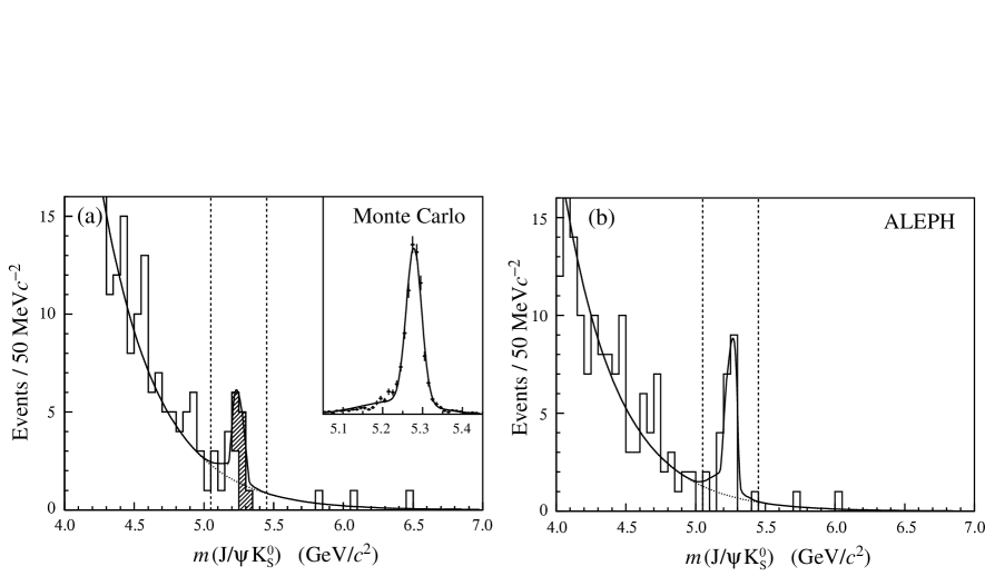
Figure 1: Reconstructed $\rm J/\psi\,K^{0}_{S}$ mass (a) for hadronic Monte Carlo, (b) for the data; the superimposed fits are described in the text, and the dashed lines indicate the signal region. In (a) the events that truly originated from a $\rm B^{0}\rightarrow J/\psi\,K^{0}_{S}$ decay are shaded, and the insert shows the mass distribution for a large sample of signal Monte Carlo events.

Next the $\rm K^{0}_{S}\rightarrow\pi^{+}\pi^{-}$ reconstruction is performed, as described in [16]. The distance of closest approach of the two daughters must be less than 5 mm, and the $dE/dx$ for each daughter is required to be within three standard deviations of the expected value for a pion. The angle between the reconstructed directions of the $\rm K^{0}_{S}$ and $\rm J/\psi$ is required to satisfy $\cos\theta_{\rm\psi K}>0.85$, and the resultant of their momenta must satisfy $p_{\rm B}>22$ GeV$/c$. The reconstructed $\rm K^{0}_{S}$ invariant mass is required to be within 15 MeV$/c^{2}$ of its nominal value.

A fit is made for the $\rm B^{0}$ decay vertex, using the two lepton tracks and the $\rm K^{0}_{S}$. The vertex is required to be successfully reconstructed, and the decay length is determined from the distance between the production and decay vertices, projected along the momentum vector of the $\rm B^{0}$ candidate. The decay length is required to be greater than $-1$ mm, and its calculated error less than 1 mm. Finally, the $\rm J/\psi\,K^{0}_{S}$ invariant mass is calculated, assigning the nominal masses to the two particles. The resulting distribution is shown as an insert in Fig. 1 (a) for signal Monte Carlo. The peak is fitted with the sum of two Gaussian functions, the first accounting for 72% of the events with a width of 20 MeV$/c^{2}$ and the second with width 90 MeV$/c^{2}$, offset to lower mass by 50 MeV$/c^{2}$. The signal region is defined as 5.05–5.45 GeV$/c^{2}$, and the overall reconstruction efficiency is 28%.

When the event selection is applied to the hadronic Monte Carlo sample, the resulting $\rm J/\psi\,K^{0}_{S}$ mass distribution is shown in Fig 1 (a). There are 20 events in the signal region, of which 11 are from background. The superimposed fit is the sum of an exponential shape to describe the background and the signal shape discussed above. The four fitted parameters are the background slope and normalization, and the signal mass and normalization.

The mass distribution that results when the event selection is applied to the data is shown in Fig. 1 (b). A clear signal is seen for the $\rm B^{0}$, with 23 events in the signal region. A fit similar to that of the hadronic Monte Carlo is made, giving a fitted $\rm B^{0}$ mass of $5.26\pm 0.01$ GeV$/c^{2}$, slightly lower than, but consistent with, the world-average value of $m_{\rm B}=5.279$ GeV$/c^{2}$. The fit is used to assign an event-by-event background probability for each event in the signal region, which is used in the maximum likelihood fit for the CP asymmetry. Their sum corresponds to 6.6 background events, giving an average background fraction $f_{\rm bkg}=0.29\pm 0.06$, where the uncertainty is estimated by varying the parametrizations within their statistical errors, and using alternative shapes for the background. The fitted shape and normalization of the background are consistent with those seen in the Monte Carlo.

After subtraction of the background, about 16 signal events remain, to be compared with the predicted number of $9\pm 2$, calculated from the expected production rate and decay branching ratios. Figure 2 shows a particularly clean signal candidate, in which there are no other charged tracks in the signal hemisphere.

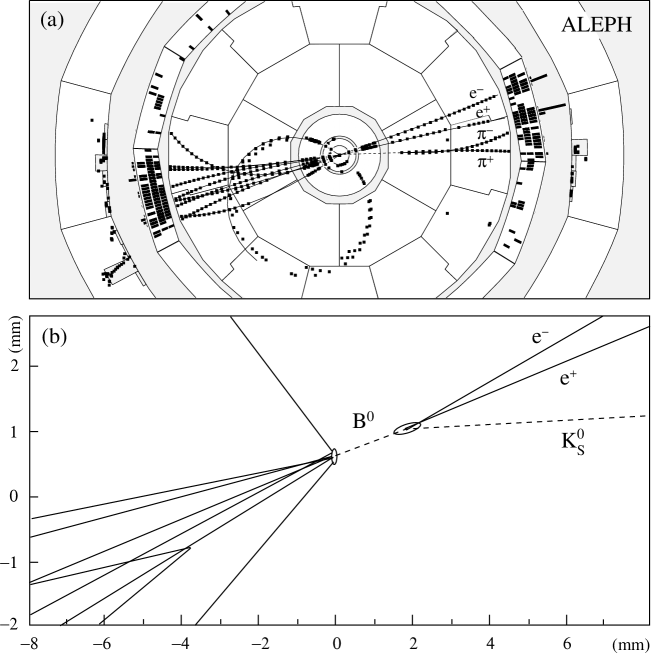
Figure 2: Event display of a $\rm B^{0}\rightarrow J/\psi\,K^{0}_{S}$ candidate in the data, with $\rm J/\psi\rightarrow e^{+}e^{-}$: (a) fish-eye view of the projection transverse to the beam axis, (b) zoom into the vertex region for the same projection, with reconstructed vertices marked with ellipses, and the reconstructed neutrals marked with dashed lines.

4 Proper-time determination

The decay length of the $\rm B^{0}$ is determined from vertex reconstruction as described in the previous section. The decay-length resolution determined using the Monte Carlo simulation is reasonably described by a Gaussian distribution of width $200\,\mu$m, although there are small tails from events with poorly measured vertices. The uncertainty on the decay length is estimated by propagating the production and decay vertex errors, which are calculated in turn from the errors of the tracks used in their determination. The pull distribution, given by the difference of true and reconstructed decay lengths divided by the calculated decay-length uncertainty, is close to being normally distributed. It has a fitted Gaussian width of 1.1, indicating that the event-by-event estimate of decay-length uncertainty is reasonably accurate.

As the signal events are fully reconstructed, the momentum resolution is excellent. There is a Gaussian core of 1% relative error, with an overall RMS of 2.5%. This small uncertainty on the momentum measurement gives a significant contribution to the overall proper-time uncertainty only for events with long decay lengths, greater than about 1 cm.

The proper time is given by $t=d_{\rm B}m_{\rm B}/p_{\rm B}$. Its uncertainty is calculated as follows:

$$\sigma_{t}=t\ \sqrt{\left(\frac{\sigma_{d}}{d_{\rm B}}\right)^{2}+\left(\frac{\sigma_{p}}{\raisebox{1.29167pt}{$p_{\rm B}$}}\right)^{2}}\ .$$ (2)

The first term in parentheses is taken from the event-by-event measurement of the decay length $d_{\rm B}$ and its error $\sigma_{d}$, scaled by a factor $1.1\pm 0.2$, where the uncertainty is taken into account for systematic studies; the second term is taken as $(2\pm 2)$%. Despite being conservative, these estimates of the uncertainty lead to a negligible effect on the measured asymmetry, as the characteristic scale of the proper-time development of the asymmetry is $1/\Delta m_{\rm d}\sim 2$ ps, much longer than the typical proper-time resolution of 0.1 ps.

Of the 11 background events in the signal region for the hadronic Monte Carlo, nine involve tracks from b-hadron decays. The apparent proper time and its error are determined for these background events, following the procedure discussed above, and a fit made for their effective lifetime $\tau_{\rm bkg}$. The probability density function is taken as the convolution of an exponential lifetime distribution with a Gaussian resolution function, and the fit gives $\tau_{\rm bkg}=1.4\ ^{+0.5}_{-0.3}$ ps.

5 Production-state tagging

The extraction of the CP asymmetry from the signal events requires the determination of whether they originated from a ${\rm B^{0}}$ or $\rm\overline{B}{}^{0}$ at production. This is achieved by studying the properties of the rest of the event, excluding the lepton and pion pairs that come from the signal $\rm B^{0}$ decay. For this purpose, two hemispheres are defined with respect to the thrust axis of the event, determined using both charged and neutral energy-flow objects [10]. These are used to separate information from the same and opposite sides of the event with respect to the ${\rm B^{0}}$ candidate. Properties of the opposite side are used to determine the particle/antiparticle nature of the other b hadron that was produced in conjunction with the signal ${\rm B^{0}}$, and thus indirectly determine its production state. The same side carries information from the fragmentation process that produced the signal ${\rm B^{0}}$, which can also be used in the production-state determination.

The calculation of the tag for the opposite side starts with the search for a secondary vertex due to b-hadron decay. This is achieved using a topological vertexing algorithm that combines information from all charged tracks in the hemisphere. Jets are reconstructed from the charged tracks and neutral energy-flow objects using the JADE algorithm [17], with a jet-resolution parameter of 0.02. The highest energy jet and the jet which forms the highest invariant mass with it are selected, and the secondary vertex is constrained to lie along the direction of the selected jet in its hemisphere, within errors. Each track is then assigned a relative probability ${\cal P}_{\rm v}$ that it originates from the secondary vertex.

Next, the b-hadron flight direction is estimated. Jets are reconstructed with a jet-resolution parameter lowered to 0.0044, as this gives an improved estimate of the b-hadron direction [15]. If more than one jet is found in the hemisphere considered, the b-jet candidate is chosen on the basis of the kinematic properties of its tracks and the presence of lepton candidates. The leading track of the b-jet candidate is then used as a seed for a second cone-based jet algorithm [18], which is taken as a first estimate of the b-hadron flight direction. In two-jet events, the thrust axis is chosen instead. The uncertainties on the reconstructed angles are parametrized from the simulation, as a function of the jet momentum. A second estimate of the direction is taken as the vector joining the primary and secondary vertices, and its error is parametrized as a function of the measured decay length. The two estimates are averaged using their parametrized errors, and the result taken as the b-hadron flight direction.

To construct the charge estimators, b-decay and fragmentation tracks must be distinguished. This is achieved by combining three variables for each track in the hemisphere: the rapidity and longitudinal momentum relative to the b-hadron flight direction, and the vertex assignment probability ${\cal P}_{\rm v}$. They are combined in a neural network, along with a hemisphere-based indicator of the quality of the inclusive vertex finding, which acts as a “control variable”. This does not directly discriminate between the b-decay and fragmentation tracks, but improves the overall performance of the neural network as the discriminating power of the other inputs vary as a function of the control variable. The single track separation output is shown in Fig. 3 (a), using neural networks trained separately for classes of tracks passing different quality criteria. The neural-network output value $x_{\rm sec}$ is converted to a probability ${\cal P}_{\rm sec}$ that the track comes from the secondary vertex. The b-hadron momentum is then determined from the sum of charged energy assigned to the secondary vertex (based on ${\cal P}_{\rm sec}$ weights), the longitudinal fraction of neutral energy in the jet, and the missing energy in the hemisphere.

Nine charge-sensitive inputs are used for the opposite-side production-state tag:

1. Jet charge ($\kappa=0.5$):

   $$Q_{\rm J}=\frac{\sum_{i}q_{i}(\mbox{\boldmath$p$}_{i}\cdot\mbox{\boldmath$d$}_{\rm J})^{\kappa}}{\sum_{i}(\mbox{\boldmath$p$}_{i}\cdot\mbox{\boldmath$d$}_{\rm J})^{\kappa}}\ ,$$ (3)

   where $i$ runs over the charged tracks in the hemisphere, $q_{i}$ and $p$_i are the charge and momentum of the track, $d$_J is the b-hadron flight direction.

2. Jet charge ($\kappa=1.0$): defined as in Eq. 3.

3. Charge of the track with highest longitudinal momentum in the hemisphere, calculated relative to the b-hadron flight direction.

4. Total charge: $Q_{\rm tot}=\sum_{i}\,q_{i}$ where $i$ runs over the charged tracks in the b jet.

5. Secondary vertex charge: ${Q_{\rm vtx}}=\sum_{i}\,{\cal P}_{\rm sec}^{i}\,q_{i}$ where $i$ runs over all charged tracks in the hemisphere.

6. Weighted primary vertex charge:

   $${Q_{\rm pri}}=\frac{\sum_{i}(1-{\cal P}_{\rm sec}^{i})\,q_{i}\,(\mbox{\boldmath$p$}_{i}\cdot\mbox{\boldmath$d$}_{\rm J})^{\kappa}}{\sum_{i}(1-{\cal P}_{\rm sec}^{i})\,(\mbox{\boldmath$p$}_{i}\cdot\mbox{\boldmath$d$}_{\rm J})^{\kappa}}\ ,$$ (4)

   where $i$ runs over all charged tracks in the hemisphere and $\kappa=1.0$.

7. Weighted secondary vertex charge: as for $Q_{\rm pri}$ but replacing $(1-{\cal P}_{\rm sec}^{i})$ with ${\cal P}_{\rm sec}^{i}$, and taking $\kappa=0.3$.

8. Decay kaon charge: kaons are identified using $dE/dx$, based upon the ratio of probabilities that the measured ionization is due to a kaon, relative to either a kaon or a pion. This variable is combined with the track momentum, longitudinal momentum and ${\cal P}_{\rm sec}$ value to select kaons from the $\rm b\rightarrow c\rightarrow s$ cascade using a further neural network. The reconstructed b-hadron momentum in the hemisphere is also used as a control variable. The charge of the track with the highest output from the neural network is used to sign the output value.

9. Lepton charge: lepton identification is performed with tighter requirements than those described previously [11]. If more than one lepton candidate is selected, that with the highest $p_{\rm T}$ with respect to the jet axis is used. The lepton transverse momentum is signed by the track charge.

Finally, six additional control variables are used: $\cos\,\theta_{\rm thrust}$, the charged track multiplicity, the spread in the measured values of ${\cal P}_{\rm sec}$: $\sigma_{\rm sec}=\sum_{i}{\cal P}_{\rm sec}\left(1-{\cal P}_{\rm sec}\right)$, the reconstructed b-hadron momentum, the reconstructed decay length, and the lepton momentum (if a lepton has been selected). These are combined along with the charge estimators using a neural network, which takes into account correlations between the variables. It provides a single output, $x_{\rm opp}$, which is shown in Fig. 3 (b).

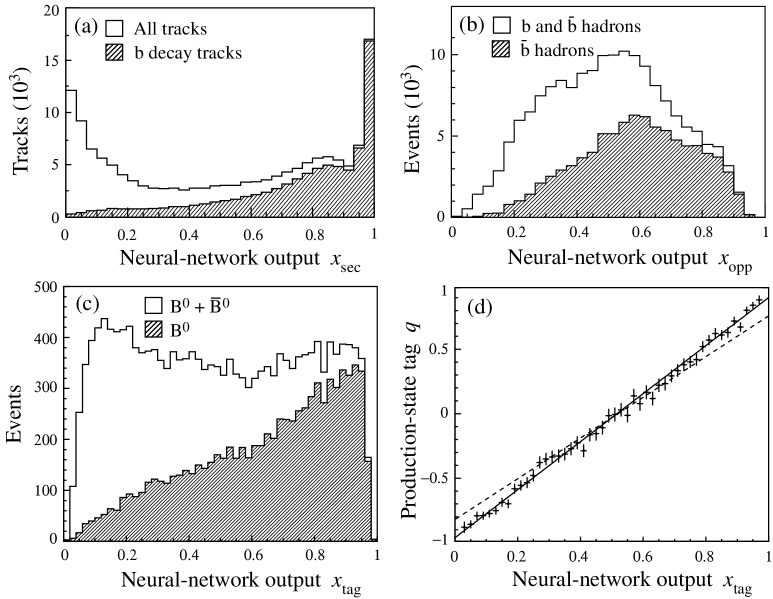
Figure 3: Neural-network output distributions for signal Monte Carlo events: (a) separation of b-decay and fragmentation tracks, $x_{\rm sec}$, with the contribution from b-decay tracks shaded; (b) opposite-side production state, $x_{\rm opp}$, with the contribution from hemispheres containing $\rm\overline{b}$ hadrons shaded; (c) overall event production state, $x_{\rm tag}$, with the contribution from $\rm B^{0}$ decays shaded. (d) Calibration of the production-state tag $q$ versus the neural-network output, with superimposed linear fit; the effect of degrading the mistag rate for systematic studies is indicated by the dashed line.

Information on the production state from the same hemisphere as the $\rm B^{0}$ candidate is limited to the charged tracks from fragmentation. Excluding the tracks from the $\rm B^{0}$, seven charge estimators are constructed using tracks coming from the primary vertex in the signal hemisphere. In a similar way to the opposite-side analysis, these include two jet charges with $\kappa$ values of 0.5 and 1.0, the charge of the track with the highest longitudinal momentum with respect to the jet, one momentum-weighted and two longitudinal-momentum-weighted primary vertex charges with $\kappa$ values of 1.0, 0.3 and 1.0, respectively, and finally the sum of track charges inside the jet. The output of the opposite-side neural network, $x_{\rm opp}$, is then combined with these same-side charge estimators and the following control variables: $\sigma_{\rm sec}$, $\cos\theta_{\rm thrust}$, and the same-side charged track multiplicity, using another neural network. The output of this event tag, $x_{\rm tag}$, is shown in Fig. 3 (c).

If events with $x_{\rm tag}>0.5$ are taken to have a ${\rm B^{0}}$ in the production state and those with $x_{\rm tag}<0.5$ to have a $\rm\overline{B}{}^{0}$, the fraction of incorrect tags (the average mistag rate) is 27.8%. The event-by-event value of the neural-network output $x_{\rm tag}$ is used in the measurement of the asymmetry. Due to its peaked distribution, seen in Fig. 3 (c), the effective mistag rate is lower than the average value quoted above. Using an overlap integral technique [19] the effective mistag rate is found to be 24.1%, measured with an independent sample of simulated events, with an expected difference of $(0.2\pm 0.2)$% between the effective mistag values for $\rm B^{0}$ and $\rm\overline{B}{}^{0}$ hemispheres. The opposite-side tag alone gives average and effective mistag rates of 31.4% and 27.6%, respectively.

Finally, the production-state tag $q$ is calculated from the neural-network output $x_{\rm tag}$, correcting for the purity in each bin of Fig. 3 (c) using

$$q=\frac{2\,F(x_{\rm tag})}{F(x_{\rm tag})+G(x_{\rm tag})}-1\ ,$$ (5)

where $F(x_{\rm tag})$ is the distribution of $x_{\rm tag}$ for events produced as $\rm B^{0}$, shaded in the figure, and $G(x_{\rm tag})$ is the distribution for $\rm\overline{B}{}^{0}$; $q=+1$ for events produced as $\rm B^{0}$ and $-1$ for $\rm\overline{B}{}^{0}$ in the case of perfect tagging. The relationship between $x_{\rm tag}$ and $q$, determined with signal Monte Carlo events, is consistent with linearity, as shown in Fig. 3 (d). It is parametrized as a straight line $q=a_{\rm tag}+2\,b_{\rm tag}(x_{\rm tag}-0.5)$, with fitted coefficients $a_{\rm tag}=-0.01\pm 0.01$ and $b_{\rm tag}=0.95\pm 0.01$.

6 Asymmetry measurement

The production-state tag $q$ is plotted against the proper time $t$ in Fig. 4 (a), for the 23 events in the signal region of the data. Considering the events which have a clear tag result, $|q|>0.5$, there are 4 “$\rm B^{0}$-like” events (positive $q$) and 9 “$\rm\overline{B}{}^{0}$-like”. Furthermore, the excess of events with negative $q$ is more noticeable with increasing proper time, as would be expected for a negative CP asymmetry.

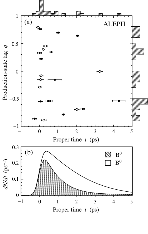
Figure 4: (a) Production-state tag $q$ versus proper time $t$ for the 23 events in the signal region of the data. The proper-time uncertainty is indicated for each point, and histograms of the two variables are shaded. The solid points indicate events with a background probability less than 30%. (b) Expected proper-time distribution of $\rm B^{0}$ and $\rm\overline{B}{}^{0}$ events, for fixed values of the CP asymmetry and proper-time resolution: $\sin 2\beta=0.7$, $\sigma_{t}=0.2$ ps.

To extract a measurement of the asymmetry, an unbinned likelihood is calculated. The probability density function expected for the signal distribution is given by

$${\cal P}_{\rm sig}(t,q)=\frac{e^{-t/\tau_{\rm d}}}{2\,\tau_{\rm d}}(1-q\,\sin 2\beta\,\sin\Delta m_{\rm d}\/t)\ .$$ (6)

The $\rm B^{0}$ lifetime $\tau_{\rm d}=1.548\pm 0.032$ ps and $\Delta m_{\rm d}=0.472\pm 0.017$ ps^-1 are fixed to the central values of their world averages [2] (the uncertainties are taken into account in systematic error studies).

A convolution is made of this signal distribution and a Gaussian resolution function ${\cal R}(\sigma_{t})$ with width given by the event-by-event proper-time resolution calculated in Section 4. The result is illustrated in Fig. 4 (b), where the contributions from $\rm B^{0}$ and $\rm\overline{B}{}^{0}$ are indicated as a function of proper time for fixed values of the asymmetry and resolution.

The probability density function for background events ${\cal P}_{\rm bkg}(t,q)$ is taken to have the same form as that of the signal but replacing $\tau_{\rm d}\rightarrow\tau_{\rm bkg}$ and $\sin 2\beta\rightarrow a_{\rm bkg}$, where the effective lifetime of the background $\tau_{\rm bkg}$ was determined in Section 4. The background asymmetry $a_{\rm bkg}$ is taken to be zero, but is varied to study possible systematic effects. The likelihood of an event is then calculated as

$${\cal L}_{i}=(1-f_{\rm bkg})\,{\cal P}_{\rm sig}(t,q)\otimes{\cal R}(\sigma_{t})+f_{\rm bkg}\,{\cal P}_{\rm bkg}(t,q)\otimes{\cal R}(\sigma_{t})\ ,$$ (7)

where $f_{\rm bkg}$ is the event-by-event background fraction discussed in Section 3. A generalized likelihood function is used, adding a Poisson term to the combined likelihoods of the signal candidates:

$$L=\frac{\nu^{n}\,e^{-\nu}}{n!}\prod_{i=1}^{n}{\cal L}_{i}\ ,$$ (8)

where $n=23$ is the number of observed candidates, and $\nu$ is the number expected.

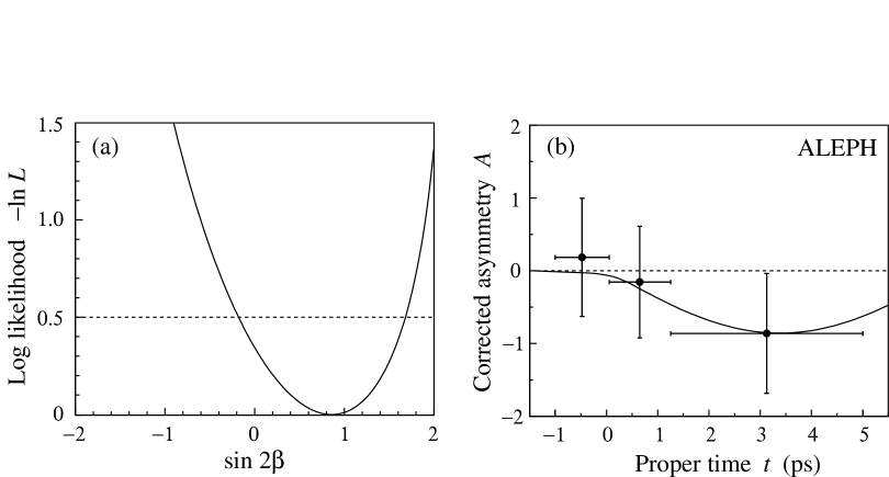
Figure 5: (a) Log-likelihood versus $\sin 2\beta$ from the fit, with respect to the minimum. (b) Reconstructed asymmetry versus proper time, after correction for the average dilution in each time bin. The result of the fit for the asymmetry is shown superimposed; note that this is not fitted directly to the binned data shown.

A fit is made with two free parameters, $\sin 2\beta$ and $\nu$, with the results $\sin 2\beta=0.84\ ^{+0.82}_{-1.04}$, $\nu=23.3\ ^{+5.1}_{-4.5}$. A scan of the log-likelihood versus $\sin 2\beta$ is shown in Fig. 5 (a). The result of the measurement is displayed as a function of proper time in Fig. 5 (b). For the purpose of display the data are divided into three proper-time bins, and the average asymmetry is corrected for the average dilution (from mistagging and background) in each bin. Negative asymmetry, and thus positive $\sin 2\beta$, is favoured.

7 Checks and systematic uncertainties

The statistical error from the fit has been checked using a fast Monte Carlo simulation. Event samples the same size as the data were generated according to Eq. 6 and 7, using the resolution function and tagging distributions discussed above. The value of $\sin 2\beta$ was set to that measured for the data, and all other parameters were fixed to their nominal values in the fit. The number of background events within the sample was varied according to Poisson statistics. The CP asymmetry of each sample was measured as if it were data, and the central value and errors recorded. This was repeated for many samples. The values reconstructed for the positive and negative errors of the data are consistent with the distributions of values seen in the simulated samples. Furthermore, the measured errors reasonably estimate the spread of the measured central value about its true input value: the pull is normally distributed.

Table 1: Contributions to the systematic uncertainty on $\sin 2\beta$.

Source	Variation	$\sigma_{\rm sys}$
$\rm B^{0}$ lifetime	$\tau_{\rm d}=1.548\pm 0.032$ ps	$<0.01$
$\rm B^{0}$ oscillation	$\Delta m_{\rm d}=0.472\pm 0.017$ ps-1	0.04
Decay-length resolution	$\sigma_{d}\times(1.1\pm 0.2)$	$<0.01$
Momentum resolution	$\Delta p/p=0.02\pm 0.02$	$<0.01$
Background level	$f_{\rm bkg}=0.29\pm 0.06$	0.09
Background lifetime	$\tau_{\rm bkg}=1.4\ ^{+0.5}_{-0.3}$ ps	0.01
Background asymmetry	$a_{\rm bkg}=0.0\pm 0.2$	0.04
Tag calibration offset	$a_{\rm tag}=-0.01\pm 0.02$	0.10
Tag calibration slope	$b_{\rm tag}=0.95\pm 0.05$	0.05
Total		0.16

The contributions to the systematic error are listed in Table 1. The lifetime and oscillation frequency of the signal were varied within their world-average uncertainties, and the effect on the measured asymmetry taken as a systematic error. For the lifetime, a check was made by fitting for the lifetime of selected signal Monte Carlo events, giving $\tau=1.56\pm 0.02$ ps, in agreement with the input value of $1.56$ ps, indicating no evidence for a systematic bias. Similarly their asymmetry was measured to be $-0.02\pm 0.03$, in agreement with the input value of zero. The decay-length and momentum resolution parametrizations were varied as discussed in Section 4.

For the background, the uncertainty on the level was discussed in Section 3. The effective lifetime of the background was varied within the large uncertainty measured using the hadronic Monte Carlo, given in Section 4. To increase the statistics for the study of the CP asymmetry of the background, events in the side-band region $4.0<m({\rm J/\psi\,K_{S}^{0}})<5.0$ GeV$/c^{2}$ were investigated. There are 140 such events in the data, with asymmetry $0.09\pm 0.23$, indicating no significant effect. About one event is expected in the signal region from the decay $\rm B^{0}\rightarrow J/\psi\,K^{*0}$ with $\rm K^{*0}\rightarrow K^{0}_{S}\,\pi^{0}$, predicted to be mainly CP even. This would correspond to a background asymmetry of less than 0.1. For the systematic error evaluation the asymmetry of the background, $a_{\rm bkg}$, was varied by $\pm 0.2$.

Uncertainties arising from the production-state tag can be considered as being due to knowledge of the overall mistag rate for signal events in data and the possible difference in the individual mistag rates for $\rm B^{0}$ and $\rm\overline{B}{}^{0}$ events. Samples of events were isolated in data with a similar topology to that of the signal, where there is a b hadron of known charge with decay products that can be cleanly separated from fragmentation tracks. Three samples of $\rm B^{+}$ candidates were selected for this purpose. The same neural network was used for tagging their production state as for $\rm B^{0}\rightarrow J/\psi\,K^{0}_{S}$, except that the sign of the same-side charge estimators is reversed. This is required as a $\overline{\rm b}$ quark combines with a d (u) quark to produce a $\rm B^{0}$ ($\rm B^{+}$), and the accompanying $\overline{\rm d}$ ($\overline{\rm u}$) quarks have opposite sign.

1. $\rm B^{+}\rightarrow J/\psi\,K^{+}$ decays: The signal selection is modified slightly, to select $\rm B^{+}\rightarrow J/\psi\,K^{+}$ decays (and charge conjugate). The reconstructed $\rm J/\psi\,K^{+}$ mass in the data is shown in Fig. 6 (a); a clear signal is seen, with 52 events in the signal region compared to an expected background of about 17. In this channel the efficiency is similar to that of $\rm J/\psi\,K^{0}_{S}$, but the product branching ratio is about three times higher. Now the charge of the kaon indicates whether the signal was produced by $\rm B^{+}$ or $\rm B^{-}$, and the resulting distributions of the neural-network output $x_{\rm tag}$ are compared in Fig. 6 (b). From a study of side-band events, the background is found to have a similar tagging distribution to the signal. The average mistag rate is 26% in signal Monte Carlo and is measured to be $(27\pm 6)$% in the data, giving confidence that the Monte Carlo simulation reproduces faithfully the features of the data used for tagging. The asymmetry and lifetime have also been measured for these events, with the results $0.09\pm 0.41$ and $1.57\ ^{+0.23}_{-0.20}$ ps, respectively. The latter agrees with the world-average value of $1.653\pm 0.028$ ps [2].

   

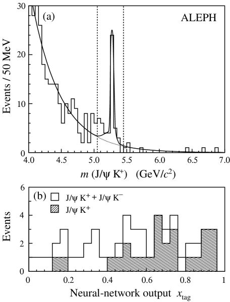
   Figure 6: (a) Reconstructed $\rm J/\psi\,K^{+}$ mass, for the data. (b) Production-state tag neural-network output $x_{\rm tag}$, when applied to events from the signal region.

2. ${\rm B}^{+}\rightarrow\overline{\rm D}{}^{0}\ell^{+}X$ decays: A selection is made of $\rm D^{0}$ candidates, decaying to a kaon and a pion of opposite charge. Only those $\rm D^{0}$ candidates are used which are found to lie in the same hemisphere as an identified lepton (e or $\mu$) with transverse momentum greater than 0.5 GeV$/c$ and charge opposite in sign to that of the pion from the $\rm D^{0}$ decay. The estimated b purity of the sample is 87%, dominated by $\rm B^{\pm}$ decays. The lepton charge indicates whether the signal was produced by a $\rm B^{+}$ or $\rm B^{-}$, and the resulting tag distributions are shown in Fig. 7 (a). The effective mistag rate determined from data is $(24.5\pm 0.6)$%, with a Monte Carlo expectation of $(24.1\pm 0.5)$%.

3. Inclusive $\rm B^{\pm}$ decays using vertex charge: A selection of $\rm B^{\pm}$ decays is made by requiring a hemisphere with $\sigma_{\rm sec}<0.32$ opposite to a b-tagged hemisphere [20], that gives an estimated b purity of 95%. A cut is then made on the absolute value of the vertex charge $|Q_{\rm vtx}|>0.6$ in the selected hemisphere, which isolates a sample containing an expected 73% of $\rm B^{\pm}$ decays. The sign of the vertex charge indicates whether the signal is produced by a $\rm B^{+}$ or a $\rm B^{-}$ and the resulting distributions of the tag output are shown in Fig. 7(b). Although significant differences are seen in this sample between the tag distributions for $\rm B^{+}$ and $\rm B^{-}$ candidates, due to material effects, they are well reproduced by the Monte Carlo. The effective mistag rate determined from data is $(21.9\pm 0.2)$%, with a Monte Carlo expectation of $(21.0\pm 0.1)$%.

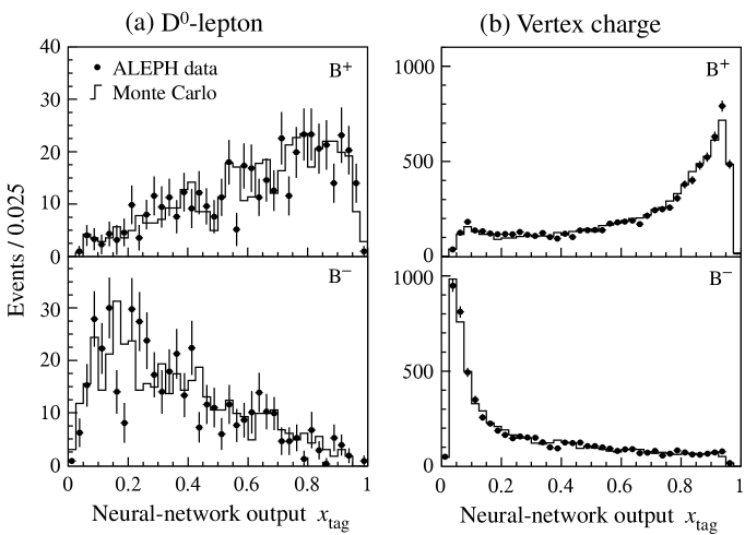
Figure 7: Production-state tag neural-network output for (a) $\rm\overline{D}{}^{0}\ell^{+}$ and (b) vertex-charge selected samples. In each figure the upper plot is for events selected as $\rm B^{+}$ candidates, the lower for $\rm B^{-}$.

The largest data-Monte Carlo disagreement for the mistag rates is $(0.9\pm 0.2)$% from the vertex-charge selected sample. In addition, separating the samples into $\rm B^{+}$ and $\rm B^{-}$ decays as shown in Fig. 7 and determining the mistag rates separately for each results in a maximum observed discrepancy of $(2.4\pm 1.3)$% from the $\rm\overline{D}{}^{0}\ell^{+}$ selected events. These are taken as systematic uncertainties for the production-state mistag rate of the $\rm B^{0}\rightarrow J/\psi\,K^{0}_{S}$ signal. Their effect is propagated to the fit for the CP asymmetry by modifying the calibration of the tag, the parametrization of $q$ versus $x_{\rm tag}$. A degraded mistag rate leads to a reduced slope of the calibration, as illustrated in Fig. 3 (d). Similarly, a $\rm B^{0}$–$\rm\overline{B}{}^{0}$ tagging difference is seen as an offset to the calibration. The variations applied to the parametrization are listed in Table 1.

Adding the systematic error contributions in quadrature, the final measurement is

$$\sin 2\beta=0.84\ ^{+0.82}_{-1.04}\pm 0.16\ ,$$ (9)

where the first error is statistical and the second systematic.

8 Conclusion

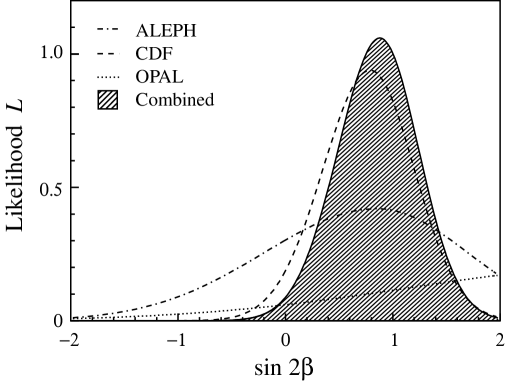
Figure 8: Likelihood distributions versus $\sin 2\beta$ for the three existing measurements (dashed lines) and their combination (shaded).

An analysis of $\rm B^{0}\rightarrow J/\psi\,K^{0}_{S}$ decays has been performed, with $\rm J/\psi\rightarrow e^{+}e^{-}$ or $\mu^{+}\mu^{-}$ and $\rm K^{0}_{S}\rightarrow\pi^{+}\pi^{-}$. A reconstruction efficiency of 28% is achieved. From the full dataset of ALEPH at LEP1 of 4.2 million hadronic Z decays, 23 candidates are selected with an estimated purity of 71%. They are used to measure the CP asymmetry of this decay, with the result $\sin 2\beta=0.84\ ^{+0.84}_{-1.05}$, where the uncertainty is dominated by the statistics.

This result is compared with the other two published measurements in Fig. 8. The likelihood of each measurement is approximated as a Gaussian distribution on either side of the central value, with width equal to the sum in quadrature of statistical and systematic errors. The three log-likelihoods can be summed to give a combined result, i.e. neglecting any correlation between the systematic errors of the different experiments (expected to be small). The resulting likelihood is shown by the shaded distribution in the figure and corresponds to $\sin 2\beta=0.88\ ^{+0.36}_{-0.39}$. The integral of the likelihood for $\sin 2\beta>0$ is 77% for the ALEPH result alone, or 67% if the total integral is limited to the physical region $|{\sin 2\beta}|<1$. The corresponding fractions are 98.6% and 98.0% for the combination of the three analyses. Thus the confidence level that CP violation has been seen in this channel is increased to 98%, compared to 93% for CDF alone [8].

Preliminary results from the BABAR and BELLE experiments [21] are consistent with the combined result given above, with similar precision and slightly lower central values.

References

- [1] M. Kobayashi and K. Maskawa, Prog. Theor. Phys. 49 (1973) 652.
- [2] Particle Data Group, D. Groom et al., Eur. Phys. J. C 15 (2000) 1.
- [3] OPAL Collaboration, K. Ackerstaff et al., “A study of B meson oscillations using inclusive lepton events in hadronic Z decays”, Z. Phys. C 76 (1997) 401; OPAL Collaboration, G. Abbiendi et al., “Measurement of the B+ and B0 lifetimes and search for CP(T) violation using reconstructed secondary vertices”, Eur. Phys. J. C 12 (2000) 609; DELPHI Collaboration, M. Feindt et al., “Study of inclusive CP(T) asymmetries in B decays”, DELPHI 97–98 CONF 80, contributed paper 449 to HEP97 Jerusalem (August 1997); ALEPH Collaboration, R. Barate et al., “Investigation of inclusive CP asymmetries in decays”, submitted to Eur. Phys. J. (July 2000).
- [4] See, for example: Y. Nir and H. Quinn, in “B Decays”, ed. S. Stone, World Scientific (1994) 362; C. Dib, I. Dunietz, F. Gilman and Y. Nir, Phys. Rev. D 41 (1990) 1522.
- [5] See, for example: A. Ali and B. Kayser, “Quark mixing and CP violation”, in “The Particle Century”, ed. Gordon Fraser, Inst. of Physics Publ. (1998) hep-ph/9806230; F. Caravaglios, F. Parodi, P. Roudeau and A. Stocchi, “Determination of the CKM unitarity triangle parameters by end 1999”, to appear in Proc. of 3rd Int. Conf. on B Physics and CP Violation (BCONF99), Taipei, Taiwan (December 1999) hep-ph/0002171.
- [6] S. Mele, Phys. Rev. D 59 (1999) 113011.
- [7] OPAL Collaboration, K. Ackerstaff et al., “Investigation of CP violation in decays at LEP”, Eur. Phys. J. C 5 (1998) 379.
- [8] CDF Collaboration, T. Affolder et al., “A Measurement of from with the CDF Detector”, Phys. Rev. D 61 (2000) 072005.
- [9] ALEPH Collaboration, D. Decamp et al., “ALEPH: a detector for electron-positron annihilations at LEP”, Nucl. Instr. Methods A 294 (1990) 121; B. Mours et al., Nucl. Instr. Methods A 379 (1996) 101.
- [10] ALEPH Collaboration, D. Buskulic et al., “Performance of the ALEPH detector at LEP”, Nucl. Instr. Methods A 360 (1995) 481.
- [11] ALEPH Collaboration, R. Barate et al., “Measurement of the and meson lifetimes”, CERN–EP/2000–106, submitted to Phys. Lett. (August 2000).
- [12] T. Sjöstrand and M. Bengtsson, Comp. Phys. Comm. 43 (1987) 367.
- [13] ALEPH Collaboration, D. Buskulic et al., “Heavy flavour production and decay with prompt leptons in the ALEPH detector”, Z. Phys. C 62 (1994) 179.
- [14] ALEPH Collaboration, R. Barate et al., “Measurement of the Z resonance parameters at LEP”, Eur. Phys. J. C 14 (2000) 1.
- [15] ALEPH Collaboration, D. Buskulic et al., “Heavy quark tagging with leptons in the ALEPH detector”, Nucl. Instr. Methods A 346 (1994) 461.
- [16] ALEPH Collaboration, D. Buskulic et al., “Production of and in hadronic Z decays”, Z. Phys. C 64 (1994) 361.
- [17] JADE Collaboration, W. Bartel et al., “Experimental studies on multijet production in annihilation at PETRA energies”, Z. Phys. C 33 (1986) 23.
- [18] OPAL Collaboration, R. Akers et al., “QCD studies using a cone-based jet finding algorithm for collisions at LEP”, Z. Phys. C 63 (1994) 197.
- [19] ALEPH Collaboration, D. Buskulic et al., “Study of the – oscillation frequency using combinations in Z decays”, Phys. Lett. B 377 (1996) 205; D. Jaffe, F. Le Diberder and M.-H. Schune, LAL 94–67 FSU–SCRI 94–101.
- [20] ALEPH Collaboration, R. Barate et al., “Search for the Standard Model Higgs boson at the LEP2 collider near GeV”, Phys. Lett. B 447 (1999) 336.
- [21] BABAR Collaboration, B. Aubert et al., “A study of time dependent CP violating asymmetries in and decays”, SLAC–PUB–8540, hep–ex/0008048 (July 2000); H. Aihara, “New results from BELLE”, presented at XXX Int. Conf. on HEP, Osaka, Japan (July 2000).