EUROPEAN ORGANIZATION FOR NUCLEAR RESEARCH

CERN-EP/2000-114

August 22, 2000

Measurement of triple gauge boson couplings from $\mathrm{W^{+}W^{-}}$ production at LEP energies up to 189 GeV

The OPAL Collaboration

Abstract

A measurement of triple gauge boson couplings is presented, based on W-pair data recorded by the OPAL detector at LEP during 1998 at a centre-of-mass energy of 189 GeV with an integrated luminosity of 183 pb^-1. After combining with our previous measurements at centre-of-mass energies of 161–183 GeV we obtain $\kappa_{\gamma}$=$0.97^{+0.20}_{-0.16}$, $g_{1}^{\mathrm{z}}$=$0.991^{+0.060}_{-0.057}$ and $\lambda$=$-0.110^{+0.058}_{-0.055}$, where the errors include both statistical and systematic uncertainties and each coupling is determined by setting the other two couplings to their Standard Model values. These results are consistent with the Standard Model expectations.

(Submitted to the European Physical Journal C)

The OPAL Collaboration

G. Abbiendi², K. Ackerstaff⁸, C. Ainsley⁵, P.F. Åkesson³, G. Alexander²², J. Allison¹⁶, K.J. Anderson⁹, S. Arcelli¹⁷, S. Asai²³, S.F. Ashby¹, D. Axen²⁷, G. Azuelos^18,a, I. Bailey²⁶, A.H. Ball⁸, E. Barberio⁸, R.J. Barlow¹⁶, S. Baumann³, T. Behnke²⁵, K.W. Bell²⁰, G. Bella²², A. Bellerive⁹, G. Benelli², S. Bentvelsen⁸, S. Bethke³², O. Biebel³², I.J. Bloodworth¹, O. Boeriu¹⁰, P. Bock¹¹, J. Böhme^14,h, D. Bonacorsi², M. Boutemeur³¹, S. Braibant⁸, P. Bright-Thomas¹, L. Brigliadori², R.M. Brown²⁰, H.J. Burckhart⁸, J. Cammin³, P. Capiluppi², R.K. Carnegie⁶, A.A. Carter¹³, J.R. Carter⁵, C.Y. Chang¹⁷, D.G. Charlton^1,b, P.E.L. Clarke¹⁵, E. Clay¹⁵, I. Cohen²², O.C. Cooke⁸, J. Couchman¹⁵, C. Couyoumtzelis¹³, R.L. Coxe⁹, A. Csilling^15,j, M. Cuffiani², S. Dado²¹, G.M. Dallavalle², S. Dallison¹⁶, A. de Roeck⁸, E. de Wolf⁸, P. Dervan¹⁵, K. Desch²⁵, B. Dienes^30,h, M.S. Dixit⁷, M. Donkers⁶, J. Dubbert³¹, E. Duchovni²⁴, G. Duckeck³¹, I.P. Duerdoth¹⁶, P.G. Estabrooks⁶, E. Etzion²², F. Fabbri², M. Fanti², L. Feld¹⁰, P. Ferrari¹², F. Fiedler⁸, I. Fleck¹⁰, M. Ford⁵, A. Frey⁸, A. Fürtjes⁸, D.I. Futyan¹⁶, P. Gagnon¹², J.W. Gary⁴, G. Gaycken²⁵, C. Geich-Gimbel³, G. Giacomelli², P. Giacomelli⁸, D. Glenzinski⁹, J. Goldberg²¹, C. Grandi², K. Graham²⁶, E. Gross²⁴, J. Grunhaus²², M. Gruwé²⁵, P.O. Günther³, C. Hajdu²⁹, G.G. Hanson¹², M. Hansroul⁸, M. Hapke¹³, K. Harder²⁵, A. Harel²¹, M. Harin-Dirac⁴, A. Hauke³, M. Hauschild⁸, C.M. Hawkes¹, R. Hawkings⁸, R.J. Hemingway⁶, C. Hensel²⁵, G. Herten¹⁰, R.D. Heuer²⁵, J.C. Hill⁵, A. Hocker⁹, K. Hoffman⁸, R.J. Homer¹, A.K. Honma⁸, D. Horváth^29,c, K.R. Hossain²⁸, R. Howard²⁷, P. Hüntemeyer²⁵, P. Igo-Kemenes¹¹, K. Ishii²³, F.R. Jacob²⁰, A. Jawahery¹⁷, H. Jeremie¹⁸, C.R. Jones⁵, P. Jovanovic¹, T.R. Junk⁶, N. Kanaya²³, J. Kanzaki²³, G. Karapetian¹⁸, D. Karlen⁶, V. Kartvelishvili¹⁶, K. Kawagoe²³, T. Kawamoto²³, R.K. Keeler²⁶, R.G. Kellogg¹⁷, B.W. Kennedy²⁰, D.H. Kim¹⁹, K. Klein¹¹, A. Klier²⁴, S. Kluth³², T. Kobayashi²³, M. Kobel³, T.P. Kokott³, S. Komamiya²³, R.V. Kowalewski²⁶, T. Kress⁴, P. Krieger⁶, J. von Krogh¹¹, T. Kuhl³, M. Kupper²⁴, P. Kyberd¹³, G.D. Lafferty¹⁶, H. Landsman²¹, D. Lanske¹⁴, I. Lawson²⁶, J.G. Layter⁴, A. Leins³¹, D. Lellouch²⁴, J. Letts¹², L. Levinson²⁴, R. Liebisch¹¹, J. Lillich¹⁰, B. List⁸, C. Littlewood⁵, A.W. Lloyd¹, S.L. Lloyd¹³, F.K. Loebinger¹⁶, G.D. Long²⁶, M.J. Losty⁷, J. Lu²⁷, J. Ludwig¹⁰, A. Macchiolo¹⁸, A. Macpherson^28,m, W. Mader³, S. Marcellini², T.E. Marchant¹⁶, A.J. Martin¹³, J.P. Martin¹⁸, G. Martinez¹⁷, T. Mashimo²³, P. Mättig²⁴, W.J. McDonald²⁸, J. McKenna²⁷, T.J. McMahon¹, R.A. McPherson²⁶, F. Meijers⁸, P. Mendez-Lorenzo³¹, W. Menges²⁵, F.S. Merritt⁹, H. Mes⁷, A. Michelini², S. Mihara²³, G. Mikenberg²⁴, D.J. Miller¹⁵, W. Mohr¹⁰, A. Montanari², T. Mori²³, K. Nagai⁸, I. Nakamura²³, H.A. Neal^12,f, R. Nisius⁸, S.W. O’Neale¹, F.G. Oakham⁷, F. Odorici², H.O. Ogren¹², A. Oh⁸, A. Okpara¹¹, M.J. Oreglia⁹, S. Orito²³, G. Pásztor^8,j, J.R. Pater¹⁶, G.N. Patrick²⁰, J. Patt¹⁰, P. Pfeifenschneider^14,i, J.E. Pilcher⁹, J. Pinfold²⁸, D.E. Plane⁸, B. Poli², J. Polok⁸, O. Pooth⁸, M. Przybycień^8,d, A. Quadt⁸, C. Rembser⁸, P. Renkel²⁴, H. Rick⁴, N. Rodning²⁸, J.M. Roney²⁶, S. Rosati³, K. Roscoe¹⁶, A.M. Rossi², Y. Rozen²¹, K. Runge¹⁰, O. Runolfsson⁸, D.R. Rust¹², K. Sachs⁶, T. Saeki²³, O. Sahr³¹, E.K.G. Sarkisyan²², C. Sbarra²⁶, A.D. Schaile³¹, O. Schaile³¹, P. Scharff-Hansen⁸, M. Schröder⁸, M. Schumacher²⁵, C. Schwick⁸, W.G. Scott²⁰, R. Seuster^14,h, T.G. Shears^8,k, B.C. Shen⁴, C.H. Shepherd-Themistocleous⁵, P. Sherwood¹⁵, G.P. Siroli², A. Skuja¹⁷, A.M. Smith⁸, G.A. Snow¹⁷, R. Sobie²⁶, S. Söldner-Rembold^10,e, S. Spagnolo²⁰, M. Sproston²⁰, A. Stahl³, K. Stephens¹⁶, K. Stoll¹⁰, D. Strom¹⁹, R. Ströhmer³¹, L. Stumpf²⁶, B. Surrow⁸, S.D. Talbot¹, S. Tarem²¹, R.J. Taylor¹⁵, R. Teuscher⁹, M. Thiergen¹⁰, J. Thomas¹⁵, M.A. Thomson⁸, E. Torrence⁹, S. Towers⁶, D. Toya²³, T. Trefzger³¹, I. Trigger⁸, Z. Trócsányi^30,g, E. Tsur²², M.F. Turner-Watson¹, I. Ueda²³, B. Vachon${26}$, P. Vannerem¹⁰, M. Verzocchi⁸, H. Voss⁸, J. Vossebeld⁸, D. Waller⁶, C.P. Ward⁵, D.R. Ward⁵, P.M. Watkins¹, A.T. Watson¹, N.K. Watson¹, P.S. Wells⁸, T. Wengler⁸, N. Wermes³, D. Wetterling¹¹ J.S. White⁶, G.W. Wilson¹⁶, J.A. Wilson¹, T.R. Wyatt¹⁶, S. Yamashita²³, V. Zacek¹⁸, D. Zer-Zion^8,l

¹School of Physics and Astronomy, University of Birmingham, Birmingham B15 2TT, UK
²Dipartimento di Fisica dell’ Università di Bologna and INFN, I-40126 Bologna, Italy
³Physikalisches Institut, Universität Bonn, D-53115 Bonn, Germany
⁴Department of Physics, University of California, Riverside CA 92521, USA
⁵Cavendish Laboratory, Cambridge CB3 0HE, UK
⁶Ottawa-Carleton Institute for Physics, Department of Physics, Carleton University, Ottawa, Ontario K1S 5B6, Canada
⁷Centre for Research in Particle Physics, Carleton University, Ottawa, Ontario K1S 5B6, Canada
⁸CERN, European Organisation for Nuclear Research, CH-1211 Geneva 23, Switzerland
⁹Enrico Fermi Institute and Department of Physics, University of Chicago, Chicago IL 60637, USA
¹⁰Fakultät für Physik, Albert Ludwigs Universität, D-79104 Freiburg, Germany
¹¹Physikalisches Institut, Universität Heidelberg, D-69120 Heidelberg, Germany
¹²Indiana University, Department of Physics, Swain Hall West 117, Bloomington IN 47405, USA
¹³Queen Mary and Westfield College, University of London, London E1 4NS, UK
¹⁴Technische Hochschule Aachen, III Physikalisches Institut, Sommerfeldstrasse 26-28, D-52056 Aachen, Germany
¹⁵University College London, London WC1E 6BT, UK
¹⁶Department of Physics, Schuster Laboratory, The University, Manchester M13 9PL, UK
¹⁷Department of Physics, University of Maryland, College Park, MD 20742, USA
¹⁸Laboratoire de Physique Nucléaire, Université de Montréal, Montréal, Quebec H3C 3J7, Canada
¹⁹University of Oregon, Department of Physics, Eugene OR 97403, USA
²⁰CLRC Rutherford Appleton Laboratory, Chilton, Didcot, Oxfordshire OX11 0QX, UK
²¹Department of Physics, Technion-Israel Institute of Technology, Haifa 32000, Israel
²²Department of Physics and Astronomy, Tel Aviv University, Tel Aviv 69978, Israel
²³International Centre for Elementary Particle Physics and Department of Physics, University of Tokyo, Tokyo 113-0033, and Kobe University, Kobe 657-8501, Japan
²⁴Particle Physics Department, Weizmann Institute of Science, Rehovot 76100, Israel
²⁵Universität Hamburg/DESY, II Institut für Experimental Physik, Notkestrasse 85, D-22607 Hamburg, Germany
²⁶University of Victoria, Department of Physics, P O Box 3055, Victoria BC V8W 3P6, Canada
²⁷University of British Columbia, Department of Physics, Vancouver BC V6T 1Z1, Canada
²⁸University of Alberta, Department of Physics, Edmonton AB T6G 2J1, Canada
²⁹Research Institute for Particle and Nuclear Physics, H-1525 Budapest, P O Box 49, Hungary
³⁰Institute of Nuclear Research, H-4001 Debrecen, P O Box 51, Hungary
³¹Ludwigs-Maximilians-Universität München, Sektion Physik, Am Coulombwall 1, D-85748 Garching, Germany
³²Max-Planck-Institute für Physik, Föhring Ring 6, 80805 München, Germany

^a and at TRIUMF, Vancouver, Canada V6T 2A3
^b and Royal Society University Research Fellow
^c and Institute of Nuclear Research, Debrecen, Hungary
^d and University of Mining and Metallurgy, Cracow
^e and Heisenberg Fellow
^f now at Yale University, Dept of Physics, New Haven, USA
^g and Department of Experimental Physics, Lajos Kossuth University, Debrecen, Hungary
^h and MPI München
ⁱ now at MPI für Physik, 80805 München
^j and Research Institute for Particle and Nuclear Physics, Budapest, Hungary
^k now at University of Liverpool, Dept of Physics, Liverpool L69 3BX, UK
^l and University of California, Riverside, High Energy Physics Group, CA 92521, USA
^m and CERN, EP Div, 1211 Geneva 23.

1 Introduction

W-pair production in $\mathrm{e^{+}e^{-}}$ annihilation involves, in addition to the $t$-channel $\nu$-exchange, the triple gauge boson vertices WW$\gamma$ and WWZ which are present in the Standard Model due to its non-Abelian nature. Since the start of LEP operation at and above the W-pair threshold several measurements have been made of the triple gauge boson couplings (TGCs) involved with these vertices in W-pair production [1, 2, 3, 4], single W and single photon production [5]. Limits on TGCs also exist from studies of di-boson production at the Tevatron [6]. In this paper we update our previous measurements [1, 2, 3] to include the data collected during 1998 at a centre-of-mass energy of 189 GeV with an integrated luminosity of $183~{}\,\mbox{pb${}^{-1}$}$.

According to the most general Lorentz invariant Lagrangian [7, 8, 9, 10] there can be seven independent couplings describing each of the WW$\gamma$ and WWZ vertices. This large parameter space can be reduced by requiring the Lagrangian to satisfy electromagnetic gauge invariance and charge conjugation as well as parity invariance. The number of parameters reduces to five, which can be taken as $g_{1}^{\mathrm{z}}$, $\kappa_{\mathrm{z}}$, $\kappa_{\gamma}$, $\lambda_{\mathrm{z}}$ and $\lambda_{\gamma}$ [7, 8]. These parameters are directly related to the W electromagnetic and weak properties [8, 9]. In the Standard Model  $g_{1}^{\mathrm{z}}$=$\kappa_{\mathrm{z}}$=$\kappa_{\gamma}$=1 and $\lambda_{\mathrm{z}}$=$\lambda_{\gamma}$=0. Precision measurements on the ${\mathrm{Z}^{0}}$ resonance and lower energy data, are consistent with the following SU(2)$\times$U(1) relations between the five couplings [7, 9],

$$\Delta\kappa_{\mathrm{z}} = -\mbox{$\Delta\kappa_{\gamma}$}\mbox{$\tan^{2}\theta_{w}$}+\mbox{$\Delta g_{1}^{\mathrm{z}}$},$$

$$\lambda_{\mathrm{z}} = \mbox{$\lambda_{\gamma}$}.$$

Here $\Delta$ indicates a deviation of the respective quantity from its Standard Model  value and $\theta_{w}$ is the weak mixing angle. These two relations leave only three independent couplings, $\Delta\kappa_{\gamma}$, $\Delta g_{1}^{\mathrm{z}}$ and $\lambda$(=$\lambda_{\gamma}$=$\lambda_{\mathrm{z}}$) which are not significantly restricted [11, 12] by existing LEP and SLC ${\mathrm{Z}^{0}}$ data.

Anomalous TGCs give different contributions to different helicity states of the outgoing W-bosons. Consequently they affect the angular distributions of the produced W bosons and their decay products, as well as the total W-pair cross-section. Ignoring the effects of the finite W width and the initial state radiation (ISR), the production and decay of W bosons is completely described by five angles. Conventionally these are taken to be [7, 9, 13]: the $\mathrm{W^{-}}$ production polar angle $\theta_{W}$; the polar and azimuthal angles, $\theta_{1}^{*}$ and $\phi_{1}^{*}$, of the decay fermion from the $\mathrm{W^{-}}$ in the $\mathrm{W^{-}}$ rest frame; and the analogous angles for the anti-fermion from the $\mathrm{W^{+}}$ decay, $\theta_{2}^{*}$ and $\phi_{2}^{*}$. However for W-pairs observed in the detector, the experimental accessibility of these angles and therefore the sensitivity to the TGCs, is limited and depends strongly on the final state produced when the W bosons decay.

In this study all final states are used, namely the fully leptonic, $\ell\overline{\nu}_{\ell}$$\overline{\ell}^{\prime}\nu_{\ell^{\prime}}$, the semileptonic, $\mathrm{q\overline{q}}$$\ell\overline{\nu}_{\ell}$, and the fully hadronic, $\mathrm{q\overline{q}}$$\mathrm{q\overline{q}}$ final states, with branching fractions of 10.6%, 43.9% and 45.6% respectively. This study is divided into two parts. In the first part the W-pair event rate for each of the three final states is analysed in terms of the TGCs. The second part is a study of the W-pair event shape for each final state using optimal observables.

Most of the TGC results of this analysis are obtained for each of the three couplings separately, setting the other two couplings to their Standard Model values. These results will be presented in tables and $\log L$ curves. We also perform two-dimensional and three-dimensional fits, where two or all three TGC parameters are allowed to vary in the fits. The results of these fits will be presented by contour plots.

The following section includes a short presentation of the OPAL data and Monte Carlo samples and in section 3 the analysis of the W-pair event rate is described. Moving on to the event shape analysis, the first step, namely the event reconstruction, is presented in section 4. The TGC extraction using the technique of optimal observables is explained in section 5. Systematic errors are described in section 6 and the combined TGC results are presented in section 7. Section 8 summarises the results of this study.

2 Data and Monte Carlo models

The data were acquired during 1998 with the OPAL detector which is described in detail elsewhere [14]. The integrated luminosity, evaluated using small angle Bhabha scattering events observed in the silicon tungsten forward calorimeter, is 183.05 $\pm$ 0.40 pb^-1. The luminosity-weighted mean centre-of-mass energy for the data sample is $\sqrt{s}$=188.64$\pm$0.04 $\mathrm{GeV}$.

In the analyses described below, a number of Monte Carlo models are used to provide estimates of efficiencies and backgrounds as well as the expected W-pair production and decay angular distributions for different TGC values. The majority of the Monte Carlo samples were generated at $\sqrt{s}$ = 189 GeV with $\mbox{$M_{\mathrm{W}}$}=80.33$ $\mathrm{GeV}\!/\!{\it c}^{2}$. All Monte Carlo samples mentioned below were processed by the full OPAL simulation program [15] and then subjected to the same reconstruction procedure as the data.

The main Monte Carlo program used in this analysis is the Excalibur [16] generator. This program generates all four-fermion final states using the full set of electroweak diagrams including the $\mathrm{W^{+}W^{-}}$ production diagrams (class CC03) and other four-fermion graphs, such as $\mbox{$\mathrm{e^{+}e^{-}}$}\rightarrow\mathrm{W}\mbox{$\mathrm{e\overline{\nu}_{e}}$}$, $\mbox{$\mathrm{e^{+}e^{-}}$}\rightarrow\mbox{${\mathrm{Z}^{0}}$}\mbox{$\mathrm{e^{+}e^{-}}$}$ and $\mbox{$\mathrm{e^{+}e^{-}}$}\rightarrow\mbox{${\mathrm{Z}^{0}}$}\mbox{${\mathrm{Z}^{0}}$}$. Using this program, samples were generated with and without anomalous TGCs. Each sample was generated with a different set of TGC values. These samples are used to calculate the TGC dependence of the expected event rate and angular distributions. We also apply a reweighting technique based on the matrix element corresponding to all the contributing four-fermion diagrams. In this way, the angular distributions for any particular set of anomalous couplings are obtained from Monte Carlo samples generated at a limited number of different TGC values.

For systematic studies we use Standard Model four-fermion samples generated by the grc4f [17] and Koralw [18] programs. Koralw uses the same matrix element as grc4f but has the most complete simulation of ISR out of all the four-fermion Monte Carlo programs used in this analysis. The efficiency obtained from the Koralw sample is used to correct the expected event rate. To estimate the hadronisation systematics, Monte Carlo samples were produced by grc4f including the CC03 diagrams only, and the fragmentation stage was generated separately with either Jetset [19] or Herwig [20]. To study final state interaction effects in $\mathrm{q\overline{q}}$$\mathrm{q\overline{q}}$ events we used Monte Carlo samples with different implementations of Bose-Einstein correlations and colour reconnection effects, as detailed in section 6.

There are other background sources not associated with four-fermion processes. The main one, $\mbox{${\mathrm{Z}^{0}}$}/\gamma\rightarrow\mbox{$\mathrm{q\overline{q}}$}$, including higher order QCD diagrams, is simulated using Pythia, with Herwig used as an alternative to study possible systematic effects. Other background processes involving two fermions in the final state are studied using Koralz [21] for $\mathrm{e}^{+}\mathrm{e}^{-}$$\rightarrow$$\mu^{+}\mu^{-}$, $\mathrm{e}^{+}\mathrm{e}^{-}$$\rightarrow$$\tau^{+}\tau^{-}$ and $\mathrm{e}^{+}\mathrm{e}^{-}$$\rightarrow$$\nu\overline{\nu}$, and Bhwide[22] for $\mathrm{e}^{+}\mathrm{e}^{-}$$\rightarrow$$\mathrm{e}^{+}\mathrm{e}^{-}$. Backgrounds from two-photon processes are evaluated using Pythia, Herwig, Phojet [23] and the Vermaseren generator[24]. It is assumed that the centre-of-mass energy of 189 $\mathrm{GeV}$ is below the threshold for Higgs boson production.

3 Event rate TGC analysis

The event rate analysis is based on the total $\mathrm{W^{+}W^{-}}$ production cross-section measurement [25]. We use here the same selection with the same efficiency and background estimates. The difference is only in the physics interpretation. To analyse the $\mathrm{W^{+}W^{-}}$ event rate, all three final states are used. Each final state corresponds to a different selection algorithm. These algorithms are similar to those used at lower centre-of-mass energies (see [3] and references therein) and the differences are described in [25].

The results are summarised in Table 1. The efficiencies refer to CC03 $\mathrm{W^{+}W^{-}}$ events and include cross contamination between the three final states. To calculate the expected numbers of events we use our total integrated luminosity of $183.05\pm 0.40$ pb^-1 and the total $\mathrm{W^{+}W^{-}}$ production cross-section value of 16.26 pb corresponding to our centre-of-mass energy of 188.64$\pm$0.04 GeV and a W mass of $M_{\mathrm{W}}$=80.42$\pm$0.07 $\mathrm{GeV}\!/\!{\it c}^{2}$ measured at the Tevatron [26]. The cross-section calculation is done using the RacoonWW [27] and YfsWW3 [28] Monte Carlo programs which include the most complete ${\cal O}(\alpha)$ radiative corrections using the double pole approximation method. The results obtained by these two independent programs agree within 0.1% [29]. Furthermore the theoretical uncertainty of 0.42% is improved compared with the 2% uncertainty of the Gentle [30] semi-analytic program which has been used in our previous publications. However, since we have not yet been able to study the full effect of our selection cuts with these recent Monte Carlo generators, we prefer not to reduce our assumed theoretical uncertainty of 2% which has only a negligible effect on our final results.

Selected as	$\mathrm{W^{+}W^{-}}$$\rightarrow$ $\ell\overline{\nu}_{\ell}$$\overline{\ell}^{\prime}\nu_{\ell^{\prime}}$	$\mathrm{W^{+}W^{-}}$$\rightarrow$ $\mathrm{q\overline{q}}$$\ell\overline{\nu}_{\ell}$	$\mathrm{W^{+}W^{-}}$$\rightarrow$ $\mathrm{q\overline{q}}$$\mathrm{q\overline{q}}$	Combined
Efficiency [%]	82.3$\pm$1.2	87.7$\pm$0.9	86.5$\pm$0.8	86.6$\pm$0.6
Signal events	258$\pm$6	1145$\pm$26	1175$\pm$26	2578$\pm$55
Background events:
4-fermion, TGC-dep.	17$\pm$2	27$\pm$4	10$\pm$6	54$\pm$7
4-fermion, TGC-indep.	7.0$\pm$0.3	34$\pm$3	71$\pm$10	111$\pm$9
$\mbox{${\mathrm{Z}^{0}}$}/\gamma\rightarrow\mbox{$\mathrm{f\overline{f}}$}$	4.1$\pm$0.3	48$\pm$6	245$\pm$17	297$\pm$17
Two-photon	0.9$\pm$0.9	3$\pm$3	0	4$\pm$4
Total background	29$\pm$3	112$\pm$9	325$\pm$21	466$\pm$24
Total expected	287$\pm$7	1257$\pm$27	1500$\pm$33	3044$\pm$60
Observed	276	1246	1546	3068

Table 1: Expected and observed numbers of events in each $\mathrm{W^{+}W^{-}}$ final state for an integrated luminosity of $183.05\pm 0.40$ pb^-1 at $188.64\pm 0.04$ $\mathrm{GeV}$, assuming $\mbox{$M_{\mathrm{W}}$}=80.42\pm 0.07$ $\mathrm{GeV}\!/\!{\it c}^{2}$ and Standard Model branching fractions. The efficiency values and the numbers of signal events include cross contamination between the three final states. The errors on the combined numbers account for correlations between the systematic errors for different final states.

The four-fermion background is split between final states with and without contributions from diagrams containing a triple gauge boson vertex. For each of the three final states in our signal the TGC-dependent background is calculated from the difference between the accepted four-fermion cross-section (including all diagrams) and the accepted CC03 cross-section. The background from other final states does not depend on the TGCs.

The errors listed in Table 1 are due to Monte Carlo statistics, luminosity uncertainty of 0.2%, theoretical uncertainty in the total cross-section (2%), centre-of-mass energy and W mass uncertainties (0.04% of the total cross-section each), data/MC differences, tracking losses, detector occupancy and fragmentation uncertainties. A detailed description of all these sources can be found in [25].

The total number of expected events in each final state is consistent with the corresponding number of observed events. Therefore, there is no evidence for any significant contribution from anomalous couplings. A quantitative study of TGCs from the W-pair event yield is performed by comparing the numbers of observed events in each of the three event selection channels with the expected numbers which are parametrised as second-order polynomials in the TGCs. This parametrisation is based on the linear dependence of the triple gauge vertex Lagrangian on the TGCs, corresponding to a second-order polynomial dependence of the cross-section. Consequently, the expected number of events for each final state also has a second-order polynomial dependence on the TGCs. The polynomial coefficients are calculated from the expected number of events at different TGC values, as obtained from the corresponding Excalibur Monte Carlo samples. For each final state, the corresponding expected cross section is normalised to the Standard Model expectation (sum of signal and TGC-dependent background) listed in Table 1. The primary reason for this normalisation is the fact that when calculating the numbers in Table 1, RacoonWW and YfsWW3 are used for the cross-section and Koralw for the efficiency. This is considered to be more complete than Excalibur. The normalisation factor varies between 0.970 ($\ell\overline{\nu}_{\ell}$$\overline{\ell}^{\prime}\nu_{\ell^{\prime}}$ selection) and 0.987 ($\mathrm{q\overline{q}}$$\mathrm{q\overline{q}}$ selection).

The probability to observe the measured number of candidates, given the expected value, is calculated using a Poisson distribution. The product of the three probability distributions corresponding to the three final states is taken as the event rate likelihood function. The systematic uncertainties are incorporated into the TGC fit by allowing the expected numbers of signal and background events to vary in the fit and constraining them to have a Gaussian distribution around their expected values with their systematic errors taken as the width of the distributions. The systematic uncertainties, excluding those on efficiency and background, are assumed to be correlated between the three different event selections.

Data from lower centre-of-mass energies are included, assuming all systematic errors to be fully correlated between energies. The corresponding $\log L$ curves are used in combination with the results of the event shape analysis, which is described in the following sections. The full set of results is then presented in Figure 7, where the event rate contributions are shown as dotted lines.

4 Event reconstruction

Starting from the event sample used for the event-rate analysis, a reconstruction is performed to extract the maximum possible information on the W production and decay angles, which are then used to extract the couplings. Events which cannot be well reconstructed are rejected from the sample.

Three kinematic fits with different sets of requirements are used in the event reconstruction:

• requiring conservation of energy and momentum, neglecting ISR;

• additionally constraining the reconstructed masses of the two W-bosons to be equal;

• additionally constraining each reconstructed W mass to the average value measured at the Tevatron, $M_{\mathrm{W}}$=80.42 $\mathrm{GeV}\!/\!{\it c}^{2}$ [26].

For $\mathrm{q\overline{q}}$$\mathrm{q\overline{q}}$ events, where all four final state fermions are measurable, fits A, B and C have 4, 5 and 6 constraints respectively. For $\mathrm{q\overline{q}}$$\mathrm{e\overline{\nu}_{e}}$ and $\mathrm{q\overline{q}}$$\mu\overline{\nu}_{\mu}$ events the number of constraints is reduced by 3 due to the invisible neutrino. For $\mathrm{q\overline{q}}$$\tau\overline{\nu}_{\tau}$ events there is at least one additional unobserved neutrino from the $\tau$ decay, but the momentum sum of the track(s) assigned to the $\tau$ can still be used as an approximation to the $\tau$ flight direction, relying on its high boost. The $\tau$ energy is left unknown, resulting in a further loss of one constraint. Finally for $\ell\overline{\nu}_{\ell}$$\overline{\ell}^{\prime}\nu_{\ell^{\prime}}$ events, where none of the leptons is a $\tau$, there are two invisible neutrinos. Hence, six constraints are lost and requirement C is needed.

In the following we discuss the reconstruction of each final state separately.

4.1 Reconstruction of $\mathrm{q\overline{q}}$$\ell\overline{\nu}_{\ell}$ final states

Candidate $\mathrm{q\overline{q}}$$\mathrm{e\overline{\nu}_{e}}$ and $\mathrm{q\overline{q}}$$\mu\overline{\nu}_{\mu}$ events without a well reconstructed lepton track, which were included in the sample used for the event rate analysis, are removed from the present sample. In this way, each of the events left in the sample has one track that is identified as the most likely lepton candidate. For the case of $\mathrm{q\overline{q}}$$\tau\overline{\nu}_{\tau}$ events, either one track or a narrow jet consisting of three tracks is assigned as the $\tau$ decay product.

The electron direction is reconstructed by the tracking detectors and the energy is measured in the electromagnetic calorimeters. For muons the momentum is measured using the tracking detectors. As explained above, the direction of $\tau$ candidates can be directly reconstructed whilst the energy can only be derived from a kinematic fit.

The remaining tracks and calorimeter clusters in the event are grouped into two jets using the Durham $k_{\perp}$ algorithm [31]. The total energy and momentum of each of the jets are calculated with the method described in [32]. Kinematic fit A, requiring energy-momentum conservation, is then performed on the events. The $\mathrm{q\overline{q}}$$\mathrm{e\overline{\nu}_{e}}$ and $\mathrm{q\overline{q}}$$\mu\overline{\nu}_{\mu}$ events are accepted if this one-constraint fit converges with a probability larger than 0.001. This cut rejects about 2% of the signal events and 4% of the background.

To improve the resolution in the angular observables used for the TGC analysis, kinematic fit C is performed on $\mathrm{q\overline{q}}$$\mathrm{e\overline{\nu}_{e}}$ and $\mathrm{q\overline{q}}$$\mu\overline{\nu}_{\mu}$ events. The W-mass constraint in this fit allows for the finite W-width. We demand that the kinematic fit converges with a probability larger than 0.001. For the 4% of events which fail at this point we revert to using the results of fit A.

For $\mathrm{q\overline{q}}$$\tau\overline{\nu}_{\tau}$ events the kinematic fit B is performed and required to converge with a probability larger than 0.025. This cut rejects 14% of the signal and 41% of the background. Furthermore, this cut suppresses those $\mathrm{q\overline{q}}$$\tau\overline{\nu}_{\tau}$ events which are correctly identified as belonging to this decay channel but where the $\tau$ decay products are not identified correctly, leading to an incorrect estimate of the $\tau$ flight direction or its charge. The fraction of such events in the $\mathrm{q\overline{q}}$$\tau\overline{\nu}_{\tau}$ sample is reduced from 18% to 12%.

Out of the original number of 1246 $\mathrm{q\overline{q}}$$\ell\overline{\nu}_{\ell}$ candidates used for the event rate analysis there are 1075 events left (368 $\mathrm{q\overline{q}}$$\mathrm{e\overline{\nu}_{e}}$, 387 $\mathrm{q\overline{q}}$$\mu\overline{\nu}_{\mu}$ and 320 $\mathrm{q\overline{q}}$$\tau\overline{\nu}_{\tau}$) after all these cuts. Assuming Standard Model cross-sections for signal and background processes, the remaining background fraction is 4.6%. This does not include cross-migration between the three lepton channels. The background sources are: four-fermion processes after subtracting the contribution from the CC03 diagrams (2.4%), $\mbox{${\mathrm{Z}^{0}}$}/\gamma\rightarrow\mbox{$\mathrm{q\overline{q}}$}$ (2.4%), $\mathrm{W^{+}W^{-}}$$\rightarrow$ $\mathrm{q\overline{q}}$$\mathrm{q\overline{q}}$ and $\ell\overline{\nu}_{\ell}$$\overline{\ell}^{\prime}\nu_{\ell^{\prime}}$ (0.2%) and two-photon reactions (0.1%).

In the reconstruction of the $\mathrm{q\overline{q}}$$\ell\overline{\nu}_{\ell}$ events we obtain $\cos\theta_{\mathrm{W}}$ by summing the kinematically fitted four-momenta of the two jets. The decay angles of the leptonically decaying W are obtained from the charged lepton four-momentum, after boosting back to the parent W rest frame. For the hadronically decaying W we are left with a two-fold ambiguity in assigning the jets to the quark and antiquark. This ambiguity is taken into account in the analyses described below.

In Figure 1 we show the distributions of all the five angles obtained from the combined $\mathrm{q\overline{q}}$$\ell\overline{\nu}_{\ell}$ event sample, and the expected distributions for $\mbox{$\Delta g_{1}^{\mathrm{z}}$}=\pm 0.5$ and 0. These expected distributions are obtained from fully simulated Monte Carlo event samples generated with Excalibur, normalised to the number of events observed in the data. Sensitivity to TGCs is observed mainly for $\cos\theta_{\mathrm{W}}$. The contribution of $\cos\theta_{\ell}^{*}$, $\phi_{\ell}^{*}$, $\cos\theta_{\scriptscriptstyle\mathrm{jet}}^{*}$ and $\phi_{\scriptscriptstyle\mathrm{jet}}^{*}$ to the overall sensitivity enters mainly through their correlations with $\cos\theta_{\mathrm{W}}$.

4.2 Reconstruction of $\mathrm{q\overline{q}}$$\mathrm{q\overline{q}}$ final states

Using the Durham $k_{\perp}$ algorithm [31], each selected $\mathrm{q\overline{q}}$$\mathrm{q\overline{q}}$ candidate is reconstructed as four jets, whose energies are corrected for the double counting of charged track momenta and calorimeter energies [33]. These four jets can be paired into W-bosons in three possible ways. To improve the resolution on the jet four-momentum we perform for each possible jet pairing the five-constraint kinematic fit B. We require at least one jet pairing with a successful fit yielding a W-mass between 70 and 90 GeV. The W charge is assigned by comparing the sum of the charges of the two jets coming from the same W candidate. More details are described in [3].

The correct di-jet pairing is identified by a likelihood algorithm [34] which takes into account correlations between the input variables. We use as input to our likelihood the W candidate mass as obtained from the kinematic fit B, the angles between the two jets coming from each W candidate, the difference between the W candidate masses as obtained from the kinematic fit A and the charge difference between the two W candidates. According to the $\mathrm{W^{+}W^{-}}$ Excalibur Monte Carlo, the probability of selecting the correct di-jet combination is about 79$\%$, and the probability of correct assignment of the W charge, once the correct pairing has been chosen, is about 77$\%$.

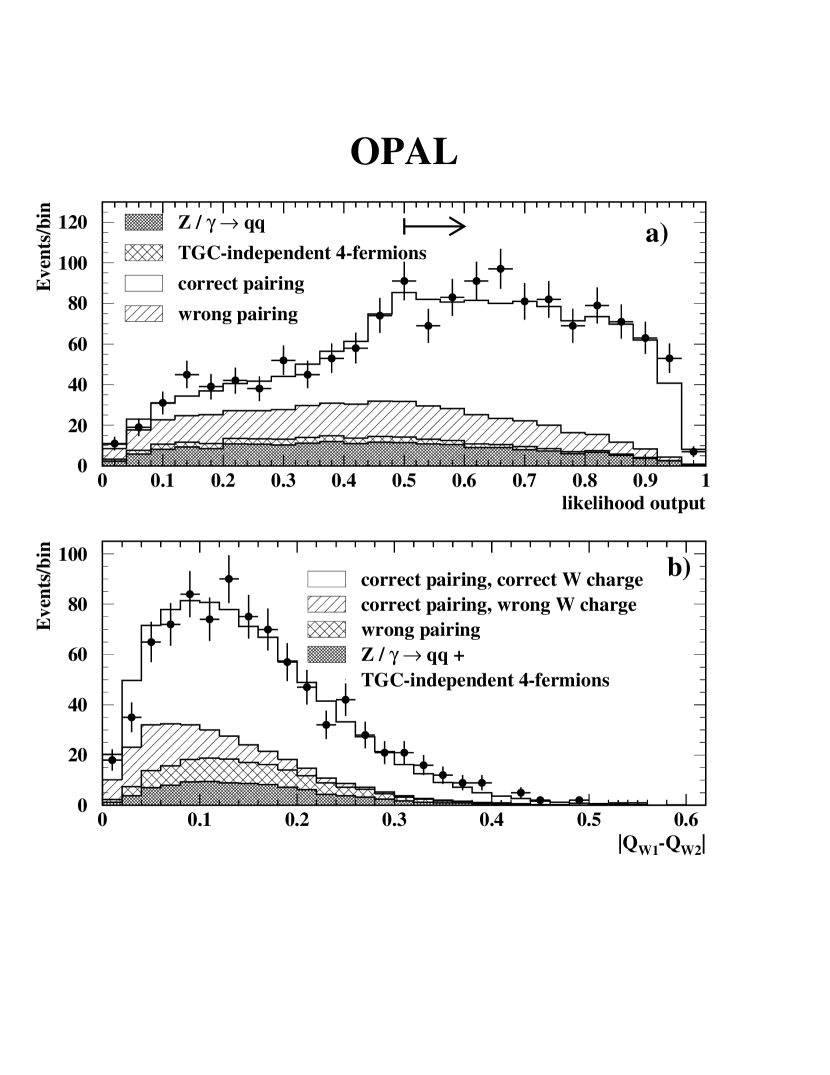
Figure 2: For the $\mathrm{q\overline{q}}$$\mathrm{q\overline{q}}$ channel, (a) distribution of the output of the jet-pairing likelihood corresponding to the most likely combination for the data (points) and for the Excalibur four-fermion Monte Carlo (histogram). The hatched area represents the contribution of wrong pairing (assuming all four quark final states compatible with W pair production are coming from such events), the double hatched area represents the contribution of the TGC-independent four-fermion background and the dark area represents the contribution of the $\mbox{${\mathrm{Z}^{0}}$}/\gamma\rightarrow\mbox{$\mathrm{q\overline{q}}$}$ background. The arrow indicates the cut value. (b) Distribution of the charge separation between the two W candidates for the data (points) and for the four-fermion Monte Carlo (histogram). The hatched area shows the contribution of correct pairing and incorrect W charge, and the double hatched area shows the contribution of wrong pairing. The dark area represents the contribution of the $\mbox{${\mathrm{Z}^{0}}$}/\gamma\rightarrow\mbox{$\mathrm{q\overline{q}}$}$ and TGC-independent four-fermion background.

The fraction of events correctly reconstructed can be increased by cutting on the value $L$ of the jet pairing likelihood. Its distribution is shown in Figure 2(a). We cut at $L>0.5$, which minimises the expected total errors on the measured TGCs.

After all cuts the probability of correct pairing increases to 87% and the probability of correct determination of the W charge is about 82%. The selection efficiency is reduced by these cuts from 86% to 54%, whereas the background drops from 23% to 12%. In the data, 889 events survive all cuts out of the 1546 initially selected. The distribution of the W charge separation is shown in Figure 2(b). The distributions of the variables $\cos\theta_{\mathrm{W}}$, $\cos\theta_{\scriptscriptstyle\mathrm{jet}}^{*}$ and $\phi_{\scriptscriptstyle\mathrm{jet}}^{*}$ are shown in Figure 3.

4.3 Reconstruction of $\ell\overline{\nu}_{\ell}$$\overline{\ell}^{\prime}\nu_{\ell^{\prime}}$ final states

As explained above, the reconstruction of $\ell\overline{\nu}_{\ell}$$\overline{\ell}^{\prime}\nu_{\ell^{\prime}}$ final states is possible only by using kinematic fit C for the case of no $\tau$-lepton in the final state. To reject events with $\tau$-leptons we use the lepton identification algorithm designed for the W branching ratio measurement [25]. In addition, events with only one reconstructed cone which were accepted for the event rate analysis are removed from the sample. As a result of these two cuts, the number of data events drops from 276 to 133. The efficiency for $\ell\overline{\nu}_{\ell}$$\overline{\ell}^{\prime}\nu_{\ell^{\prime}}$ events with $\ell=$e,$\mu$ drops from 89% to 74%. The contamination left in the sample from $\ell\overline{\nu}_{\ell}$$\overline{\ell}^{\prime}\nu_{\ell^{\prime}}$ final states with a $\tau$-lepton is 14% and the background from other final states is only 0.5%.

Kinematic fit C has no constraints and turns into solving a quadratic equation. In the ideal case of no measurement errors and satisfying the conditions where fit C is valid, namely no ISR and narrow W width, one expects to obtain two real solutions corresponding to a two-fold ambiguity in the angle set $\cos\theta_{W}$, $\phi_{1}^{*}$ and $\phi_{2}^{*}$. There is no ambiguity in the angles $\theta_{1}^{*}$ and $\theta_{2}^{*}$ which have a one-to-one correspondence with the lepton momenta. In realistic conditions, however, including ISR, finite W width and measurement errors, one might obtain no real solution, but a pair of complex conjugate solutions. In fact, only 92 out of 133 events in the data have two real solutions, in agreement with the Monte Carlo expectation of 97.8 events. In the complex solution case, the nearest real solution is taken by setting the imaginary parts of the complex solutions to zero.

Figure 4 shows the reconstructed $\cos\theta_{\mathrm{W}}$ distribution. The data distribution agrees with the Standard Model expectation.

5 Event shape TGC analysis

The angular distributions from all final states are consistent with the Standard Model expectation and no evidence is seen for any significant contributions from anomalous couplings. For a quantitative study we use the method of optimal observables based on the following dependence of the W-pair differential cross-section on the TGCs,

$$d\sigma(\Omega,\mbox{$\alpha$})=S^{(0)}(\Omega)+\sum_{i}\mbox{$\alpha$}_{i}\cdot S_{i}^{(1)}(\Omega)+\sum_{i,j}\mbox{$\alpha$}_{i}\mbox{$\alpha$}_{j}\cdot S^{(2)}_{ij}(\Omega),\ \ \ \mbox{$\alpha$}_{i}\ =\ \mbox{$\Delta\kappa_{\gamma}$},\ \mbox{$\Delta g_{1}^{\mathrm{z}}$}\ {\rm and}\ \mbox{$\lambda$},$$

where $\Omega$ are the five phase-space variables, $\Omega$=($\cos\theta_{\mathrm{W}}$,$\cos\theta_{1}^{*}$,$\phi_{1}^{*}$,$\cos\theta_{2}^{*}$,$\phi_{2}^{*}$). For this kind of dependence it has been shown [35] that all information contained in the phase-space variables $\Omega$ is retained in the whole set of nine observables $\mbox{${\cal O}$}_{i}^{(1)}=S_{i}^{(1)}(\Omega)/S^{(0)}(\Omega)$, $\mbox{${\cal O}$}_{i}^{(2)}=S_{ii}^{(2)}(\Omega)/S^{(0)}(\Omega)$ and $\mbox{${\cal O}$}_{ij}^{(2)}=\mbox{${\cal O}$}_{ji}^{(2)}=S_{ij}^{(2)}(\Omega)/S^{(0)}(\Omega)$ $(i,j=1,2,3)$.

The original idea [36, 37, 38] was to use only the mean values of the first order observables, $\mbox{$\overline{\cal O}$}^{(1)}$. However, this causes some ambiguities which can be resolved by inclusion of the mean value of the second order observables, $\mbox{$\overline{\cal O}$}^{(2)}$. For one-dimensional fits, where only one TGC parameter, $\mbox{$\alpha$}_{i}$, is allowed to vary and the others are set to their Standard Model values, we use only the corresponding first order, $\mbox{${\cal O}$}_{i}^{(1)}$, and second order, $\mbox{${\cal O}$}_{i}^{(2)}$, observables. In three-dimensional fits, where all three TGC parameters are allowed to vary, all nine observables are used.

The analysis is done separately for the $\mathrm{q\overline{q}}$$\ell\overline{\nu}_{\ell}$, $\mathrm{q\overline{q}}$$\mathrm{q\overline{q}}$ and $\ell\overline{\nu}_{\ell}$$\overline{\ell}^{\prime}\nu_{\ell^{\prime}}$ final states. The nine optimal observables are constructed for each event $k$ with the set of phase-space variables $\Omega_{k}$ using the analytic expression for the CC03 Born differential cross-section to calculate the values of $S^{(0)}(\Omega_{k}),\ S_{i}^{(1)}(\Omega_{k}),\ S_{ii}^{(2)}(\Omega_{k})$ and $S_{ij}^{(2)}(\Omega_{k})$, taking into account the reconstruction ambiguities for that particular final state. For the $\mathrm{q\overline{q}}$$\mathrm{q\overline{q}}$ channel, the uncertainty in the identity of the W⁺ and the W^- is taken into account by weighting each hypothesis with its probability, determined from the Monte Carlo as a function of the charge difference $|Q_{W_{1}}-Q_{W_{2}}|$ between the two W candidates in the event.

The expected mean values of each observable as a function of the TGCs are calculated from four-fermion Monte Carlo events generated according to the Standard Model as well as samples generated with various TGC values. The Excalibur matrix element calculation is used to reweight the Monte Carlo events to any TGC value required. The contribution of background events is also taken into account in the calculation of the expected mean values using corresponding Monte Carlo samples.

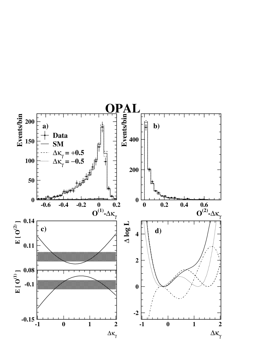
Figure 5: $\mathrm{q\overline{q}}$$\ell\overline{\nu}_{\ell}$ event distributions of the (a) first and (b) second order optimal observables corresponding to $\Delta\kappa_{\gamma}$. The histograms show the expectation of the Standard Model and when $\mbox{$\Delta\kappa_{\gamma}$}=\pm 0.5$. The expected mean values of these observables are plotted in (c) (lower and upper plot respectively) as solid curves. The measured mean values and their statistical errors are indicated by the shaded horizontal bands. In figure (d) the contributions of the first and second order optimal observable to the $\log L$ function, disregarding the correlation between them, are plotted by the dashed and dotted lines respectively. The dash-dotted line is the contribution of the correlation between the two observables and the solid line is the overall $\log L$ function which is the sum of the three contributions.

An illustrative example is shown in Figure 5 for $\mbox{${\cal O}$}_{\tiny\mbox{$\Delta\kappa_{\gamma}$}}^{(1)}$ and $\mbox{${\cal O}$}_{\tiny\mbox{$\Delta\kappa_{\gamma}$}}^{(2)}$ using the $\mathrm{q\overline{q}}$$\ell\overline{\nu}_{\ell}$ final state. Figures 5(a) and 5(b) show the distributions of these observables in the data compared with the Monte Carlo expectations at the Standard Model and at $\Delta\kappa_{\gamma}$=$\pm$0.5. The data agree with the Standard Model distributions. In Figure 5(c) the expected mean values $E[{\cal O}_{\tiny\mbox{$\Delta\kappa_{\gamma}$}}^{(1)}]$ and $E[{\cal O}_{\tiny\mbox{$\Delta\kappa_{\gamma}$}}^{(2)}]$ as functions of $\Delta\kappa_{\gamma}$ are shown along with the measured mean values $\mbox{$\overline{\cal O}$}^{(1)}_{\tiny\mbox{$\Delta\kappa_{\gamma}$}}$ and $\mbox{$\overline{\cal O}$}^{(2)}_{\tiny\mbox{$\Delta\kappa_{\gamma}$}}$.

A $\chi^{2}$ fit of the measured mean values $\overline{\cal O}$ to the corresponding expectations $E[{\cal O}]$($\alpha$) is performed to extract the couplings from the data. The covariance matrix for the mean values is calculated from the Monte Carlo events. In the calculation of the $\chi^{2}$ for the $\mathrm{q\overline{q}}$$\ell\overline{\nu}_{\ell}$ channel, the contribution of the $\mathrm{q\overline{q}}$$\tau\overline{\nu}_{\tau}$ final state is calculated separately, in order to account for the worse resolution of $\mathrm{q\overline{q}}$$\tau\overline{\nu}_{\tau}$ events compared with $\mathrm{q\overline{q}}$$\mathrm{e\overline{\nu}_{e}}$ and $\mathrm{q\overline{q}}$$\mu\overline{\nu}_{\mu}$ final states. The $\log L$ curve is obtained by subtracting from the $\chi^{2}$ function its minimum value and dividing by two. For illustration, the $\log L$ function corresponding to the one-dimensional fit to obtain $\Delta\kappa_{\gamma}$ from the $\mathrm{q\overline{q}}$$\ell\overline{\nu}_{\ell}$ data using $\mbox{${\cal O}$}_{\tiny\mbox{$\Delta\kappa_{\gamma}$}}^{(1)}$ and $\mbox{${\cal O}$}_{\tiny\mbox{$\Delta\kappa_{\gamma}$}}^{(2)}$ is shown in Figure 5(d). This $\log L$ function can be decomposed into three contributions coming from $\mbox{${\cal O}$}_{\tiny\mbox{$\Delta\kappa_{\gamma}$}}^{(1)}$, $\mbox{${\cal O}$}_{\tiny\mbox{$\Delta\kappa_{\gamma}$}}^{(2)}$ and the correlation between them. The first two contributions are defined disregarding the correlation. Each of them has two minima at equal height. Therefore, using only one of the two observables to calculate the $\log L$ function results in an ambiguous two-fold solution, whereas using both observables leaves only one solution. Figure 5(d) also demonstrates the importance of the correlation between the two observables.

The method is tested with a large number of Monte Carlo subsamples corresponding to the Standard Model and to various TGCs. The size of each subsample corresponds to the collected luminosity. Summing up the $\log L$ curves from the different subsamples corresponding to the same coupling gives results which are consistent with the coupling value used in the Monte Carlo generation. Also the distribution of the fit results is centred around the expected value, but there are some non Gaussian tails. Therefore, it is important to test the reliability of the error interval which is estimated in the usual way, to be the region where the $\log L$ function has a value of no more than 0.5. This is done by calculating the fraction of subsamples where the correct value is within the error interval. The error estimate is considered to be reliable if the calculated fraction is consistent with 68%, otherwise the $\log L$ functions corresponding to the subsamples are scaled down by the necessary factor to obtain 68% of the subsamples within the error interval. The same scale factor is then applied also on the corresponding $\log L$ function of the data. The values obtained for this scale factor are between 0.95 and 1.

	$\Delta\kappa_{\gamma}$	$\Delta g_{1}^{\mathrm{z}}$	$\lambda$
$\mathrm{q\overline{q}}$$\ell\overline{\nu}_{\ell}$
Without systematics	$-0.12^{+0.28}_{-0.21}$	$-0.029^{+0.074}_{-0.071}$	$-0.129^{+0.075}_{-0.073}$
Expected stat. uncertainty	$\pm 0.26$	$\pm 0.068$	$\pm 0.073$
Including systematics	$-0.11^{+0.30}_{-0.22}$	$-0.034^{+0.077}_{-0.073}$	$-0.125^{+0.079}_{-0.076}$
Including 161-183 GeV data	$-0.10^{+0.26}_{-0.21}$	$-0.030^{+0.068}_{-0.066}$	$-0.133^{+0.071}_{-0.068}$
Including event rate	$-0.07^{+0.25}_{-0.19}$	$-0.028^{+0.067}_{-0.065}$	$-0.125^{+0.068}_{-0.065}$
$\mathrm{q\overline{q}}$$\mathrm{q\overline{q}}$
Without systematics	$0.36^{+0.68}_{-0.46}$	$0.08^{+0.16}_{-0.14}$	$0.05^{+0.21}_{-0.16}$
Expected stat. uncertainty	$\pm 0.57$	$\pm 0.15$	$\pm 0.19$
Including systematics	$0.31^{+0.73}_{-0.51}$	$0.05^{+0.18}_{-0.15}$	$0.06^{+0.30}_{-0.20}$
Including 172-183 GeV data	$0.43^{+0.51}_{-0.43}$	$0.12^{+0.17}_{-0.14}$	$0.17^{+0.31}_{-0.20}$
Including event rate	$0.85^{+0.43}_{-1.06}$	$0.16^{+0.17}_{-0.18}$	$0.30^{+0.19}_{-0.30}$
$\ell\overline{\nu}_{\ell}$$\overline{\ell}^{\prime}\nu_{\ell^{\prime}}$
Without systematics	$-0.10^{+1.32}_{-0.37}$	$-0.04^{+0.25}_{-0.35}$	$-0.19\pm 0.15$
Expected stat. uncertainty	$\pm 0.50$	$\pm 0.27$	$\pm 0.17$
Including systematics	$-0.10^{+1.33}_{-0.37}$	$-0.04^{+0.25}_{-0.35}$	$-0.19\pm 0.15$
Including 183 GeV data	$-0.17^{+0.53}_{-0.33}$	$-0.17^{+0.28}_{-0.39}$	$-0.20\pm 0.14$
Including event rate	$-0.08^{+0.50}_{-0.31}$	$-0.09^{+0.21}_{-0.20}$	$-0.17^{+0.13}_{-0.12}$
All final states
Including systematics	$-0.03^{+0.26}_{-0.19}$	$-0.018^{+0.067}_{-0.064}$	$-0.118^{+0.066}_{-0.064}$
Including previous data	$-0.00^{+0.23}_{-0.18}$	$-0.008^{+0.059}_{-0.058}$	$-0.113^{+0.059}_{-0.057}$
Overall combined results
(including event rate)	$-0.03^{+0.20}_{-0.16}$	$-0.009^{+0.060}_{-0.057}$	$-0.110^{+0.058}_{-0.055}$
95% C.L. limits	$[-0.32,\;\;0.45]$	$[-0.12,\;\;0.11]$	$[-0.22,\;\;0.01]$
3-D fit results	$0.02^{+0.20}_{-0.15}$	$0.120^{+0.077}_{-0.083}$	$-0.190^{+0.087}_{-0.082}$

Table 2: Measured values of the TGC parameters for each final state and the results after combining all final states. For the individual final states we also list the results before including the systematic errors and the expected statistical errors. We also list the results after combining with our previous data and after combining with the event rate information from all centre-of-mass energies. For the overall combined data we list also the corresponding 95% C.L. limits. In the last row we present the results of a 3-dimensional fit to the overall combined data where all three TGC parameters are allowed to vary simultaneously.

Performing one-dimensional fits to the 189 $\mathrm{GeV}$ data, we obtain the results quoted in Table 2. The expected statistical errors, which are the average fit errors of the Monte Carlo subsamples, are also quoted in Table 2, demonstrating the different sensitivities for the various final states and TGC parameters.

As a cross-check to the mean optimal observable method, two other fit methods are applied to the $\mathrm{q\overline{q}}$$\ell\overline{\nu}_{\ell}$ events. The first one is the binned maximum likelihood method which has been used to analyse our previous data and is fully described in [1, 2]. For the present data we use a distribution in all five phase-space variables. This method yields sensitivities comparable with those of our main analysis.

The second cross-check fit for the $\mathrm{q\overline{q}}$$\ell\overline{\nu}_{\ell}$ results uses an unbinned maximum likelihood. The contribution of each data event to the likelihood is the sum over all Monte Carlo events of their weights, which are Gaussian functions of the distance in phase-space to that data event. In this way, most of the contribution comes from the Monte Carlo events nearest in phase space to the data event. The TGC dependence of the likelihood is obtained by using Monte Carlo events at different TGC values. This analysis has been applied so far only in a three-dimensional phase-space in $\cos\theta_{\mathrm{W}}$, $\cos\theta_{\ell}^{*}$ and $\phi_{\ell}^{*}$, and the obtained sensitivities are inferior to those of our main method.

For the $\mathrm{q\overline{q}}$$\mathrm{q\overline{q}}$ events our fit method is cross-checked with a binned maximum likelihood fit to the shape of the $\cos\theta_{\mathrm{W}}$ distribution as done in our previous analysis [3]. Since it uses only one phase-space variable, this method yields worse sensitivities than our main analysis.

The results of all these cross-check analyses are compatible with those of our mean value optimal observable method.

6 Study of systematics

The systematic uncertainties assigned to the event shape TGC results are listed in Table 3. The following sources are considered.

• Our analysis relies on the predictions of the Excalibur Monte Carlo generator. The grc4f and Koralw generators have a different calculation of the matrix elements and a different treatment of ISR. The associated systematic errors are assessed by applying our analysis to event samples generated with these Monte Carlo programs.

• The Monte Carlo modelling of the efficiency dependence on the event shape is checked by comparing data and Monte Carlo distributions of kinematic variables which might be affected by the selection cuts, such as the lepton and jet polar angle and energy, as well as the angle between the lepton in $\mathrm{q\overline{q}}$$\ell\overline{\nu}_{\ell}$ events and the closest jet. An agreement is found between data and Monte Carlo within the statistical errors which are used to estimate the systematic uncertainty due to this source. For the $\ell\overline{\nu}_{\ell}$$\overline{\ell}^{\prime}\nu_{\ell^{\prime}}$ final state the event statistics are not sufficient to perform this check. The uncertainty for these two charged lepton events is taken as twice the uncertainty of the $\mathrm{q\overline{q}}$$\ell\overline{\nu}_{\ell}$ events with one charged lepton. This conservative estimate is based on the assumption that the $\mathrm{q\overline{q}}$$\ell\overline{\nu}_{\ell}$ uncertainty in the efficiency is entirely related to the lepton identification.

• Uncertainties in estimating the background are determined by varying both its shape and normalisation. The shape predicted by Pythia of the $\mbox{${\mathrm{Z}^{0}}$}/\gamma\rightarrow\mbox{$\mathrm{q\overline{q}}$}$ background which is the main one for the $\mathrm{q\overline{q}}$$\ell\overline{\nu}_{\ell}$ and $\mathrm{q\overline{q}}$$\mathrm{q\overline{q}}$ final states is replaced by that predicted by Herwig. The normalisation is varied within the background uncertainty as determined in the cross-section analysis [25]. The contributions from two-photon processes are much smaller and a conservative estimate of their uncertainties is obtained by removing them from the analysis.

• The uncertainty due to jet and lepton reconstruction is investigated by considering the effects of smearing and shifting jet parameters in Monte Carlo events. The resolutions in jet energy, $\cos\theta$ and $\phi$ are varied by 10%, 5% and 3% respectively. Jet and lepton energies are shifted by 0.5% and jet $\cos\theta$ values are shifted by 0.0003. The sizes of these variations have been obtained from extensive studies of back-to-back jets in ${\mathrm{Z}^{0}}$ events collected during calibration runs. The same reconstruction uncertainties are also assumed for the $\tau$ jets in $\mathrm{q\overline{q}}$$\tau\overline{\nu}_{\tau}$ events. The momentum resolution of electrons and muons and their charge misassignment probability are modified by varying the resolution in $q/p_{\scriptscriptstyle T}$ by 10%. Here $q$ and $p_{\scriptscriptstyle T}$ are the lepton charge and transverse momentum with respect to the beam.

• The uncertainty in the beam energy of 20 MeV and the effect of our Monte Carlo samples being produced at a centre-of-mass energy 360 MeV higher than the data are investigated by applying our analysis to Monte Carlo samples generated at different centre-of-mass energies then those used for reference samples. The effect of the W-mass uncertainty is assessed in a similar way using Monte Carlo samples generated with different W-masses.

• Possible dependences on fragmentation models are studied by comparing the results of the analysis when applied to a Monte Carlo sample generated with grc4f using either Jetset or Herwig for the fragmentation phase. The main effect is on the $\mathrm{q\overline{q}}$$\mathrm{q\overline{q}}$ final state, where Herwig predicts a higher probability of correct jet pairing and correct W charge assignment than Jetset. This effect is partially due to the average charged multiplicity for u,d,s,c quarks being lower in our tuned version of Herwig than in Jetset. Since the data are in agreement with Jetset, we weight the Herwig Monte Carlo events so as to reproduce the same mean charged multiplicity as Jetset. The effect of this weighting is a reduction of the systematic error by about 25-30% for all couplings.

• Bose-Einstein correlations (BEC) in $\mathrm{q\overline{q}}$$\mathrm{q\overline{q}}$ events might affect the measured W charge distribution. We investigate this effect with a Monte Carlo program simulating BEC via re-shuffling of final state momenta [39].

• The jet reconstruction and the measured W charge distribution might also be affected by colour reconnection. This effect is investigated with several Monte Carlo samples generated according to the Ariadne [40] and Sjöstrand-Khoze [41] models. The largest effect is observed in the Ariadne 2 and Ariadne 3 models. However, these models have been disfavoured by studies of three jet events in LEP Z⁰ data [42]. For this reason the current Ariadne implementation of colour reconnection is not used to assign a systematic uncertainty. Of the remaining models considered, the Sjöstrand-Khoze model I produces the largest bias.

Source		$\mathrm{q\overline{q}}$$\ell\overline{\nu}_{\ell}$			$\mathrm{q\overline{q}}$$\mathrm{q\overline{q}}$			$\ell\overline{\nu}_{\ell}$$\overline{\ell}^{\prime}\nu_{\ell^{\prime}}$
		$\Delta\kappa_{\gamma}$	$\Delta g_{1}^{\mathrm{z}}$	$\lambda$	$\Delta\kappa_{\gamma}$	$\Delta g_{1}^{\mathrm{z}}$	$\lambda$	$\Delta\kappa_{\gamma}$	$\Delta g_{1}^{\mathrm{z}}$	$\lambda$
a)	MC generator	$0.020$	$0.001$	$0.007$	0.05	0.01	0.01	$0.13$	$0.03$	$0.02$
b)	Efficiency	$0.038$	$0.010$	$0.012$	0.03	0.01	0.02	$0.06$	$0.02$	$0.02$
c)	Background	$0.030$	$0.002$	$0.007$	0.04	0.02	0.03	$0.02$	$0.02$	$0.02$
d)	Reconstruction	$0.040$	$0.005$	$0.014$	0.01	0.01	-	$0.01$	$-$	$-$
e)	$E_{\mathrm{beam}}$ and $M_{\mathrm{W}}$	$0.021$	$0.006$	$0.014$	0.05	0.01	0.03	$0.01$	$0.01$	$0.01$
f)	Fragmentation	$0.008$	$0.012$	$0.005$	0.17	0.06	0.08	-	-	-
g)	BEC	-	-	-	0.04	0.02	0.03	-	-	-
h)	Colour reconnection	-	-	-	0.01	0.01	0.03	-	-	-
	Combined	$0.070$	$0.018$	$0.026$	0.20	0.07	0.10	$0.14$	$0.05$	$0.04$

Table 3: Contributions to the systematic uncertainties in the determination of the TGC parameters from the 189 $\mathrm{GeV}$ event shape data for different final states.

The dominant contributions to the systematic errors in different final states come from different sources, and therefore we neglect any possible correlations between the systematic errors from different final states.

The systematic uncertainties from all sources are combined in quadrature. The values in Table 3 are not directly used in the analysis. Instead we use the systematic uncertainties in the expected mean optimal observables. Correlations between the systematic errors of different observables are also taken into account and the full systematic covariance matrix is added to the statistical covariance matrix. The combined covariance matrix is used in the $\chi^{2}$ fits to obtain the TGCs. In this way, the TGC errors obtained from the fit are already the combined (statistical and systematic) errors. The results of these fits are listed in Table 2.

7 Combined TGC results

The $\log L$ functions obtained from the TGC event shape analyses including the systematic errors are combined with the curves obtained from our previous analysis at lower centre-of-mass energies [1, 2, 3]. The systematic errors from the results of the different centre-of-mass energies are assumed to be uncorrelated. This assumption does not affect the final results, since the small contribution of the systematic uncertainties to the total errors of the previous data (see Tables 8, 10 and 12 in [3]) becomes completely negligible after combining with the present results.

Table 2 lists the event shape results for each final state after combining with the previous data. The corresponding $\log L$ functions are added to those obtained from the event rate. The correlation between the systematic errors of the event rate and event shape, mainly due to the uncertainty in the background level, is neglected, as it affects the results by less than 1% of their statistical errors. The resulting $\log L$ curves are shown in Figure 6 and the corresponding TGC results are listed in Table 2.

Finally the results of the three final states are combined. This is done by first combining separately the three $\log L$ functions from the event shapes and those from the event rate. In the next step the event shape and event rate $\log L$ functions are combined into the overall result. In combining the event shape information from the three channels, the correlations between the systematic errors are neglected as already explained in section 6. On the other hand, the correlations in the event rate data are not neglected, as already mentioned in section 3. The $\log L$ curves obtained after combining the three final states are shown in Figure 7, separately for the event rate and event shape information and their sum. In Table 2 we list the TGC results obtained from the combination over the three final states of the event shape data and those after including the event rate information. The overall combined results are shown also in terms of 95% C.L. intervals.

To study correlations between the three TGC parameters we also extract a $\log L$ as a function of all three variables, $\Delta\kappa_{\gamma}$, $\Delta g_{1}^{\mathrm{z}}$ and $\lambda$. Figure 8 shows the 95% C.L. contour plots obtained from two-dimensional fits, where the third parameter is fixed at its Standard Model value. We also perform a three-dimensional fit, where all three couplings are allowed to vary simultaneously. These fit results are listed in the last row of Table 2 and the corresponding two-dimensional projections are plotted as dashed contour lines in Figure 8. As can be seen, the allowed range for each parameter is extended when the constraints on the other two parameters are removed. The different minima locations for the two- and three-dimensional fits in some of these plots, as well as their non-elliptic shape, emerge from the presence of local minima in the three-dimensional $\log L$ function [13].

8 Summary

Using a sample of 3068 $\mathrm{W^{+}W^{-}}$ candidates collected at LEP at a centre-of-mass energy of 189 $\mathrm{GeV}$, we measure the TGC parameters. For this measurement we use the event rates and event shapes of W pairs decaying into all final states. After combining our results with those obtained from the 161-183 GeV data we obtain:

$$\kappa_{\gamma} = \;\;\;\mbox{$0.97^{+0.20}_{-0.16}$},$$

$$g_{1}^{\mathrm{z}} = \;\;\;\mbox{$0.991^{+0.060}_{-0.057}$},$$

$$\lambda = \mbox{$-0.110^{+0.058}_{-0.055}$},$$

where each parameter is determined when the other two parameters are set to their Standard Model values. These results supersede those from our previous publications [1, 2, 3]. They are all consistent with the Standard Model.

Figure 1: Distributions of the kinematic variables $\cos\theta_{\mathrm{W}}$, $\cos\theta_{\ell}^{*}$, $\cos\theta_{\scriptscriptstyle\mathrm{jet}}^{*}$, $\phi_{\ell}^{*}$ and $\phi_{\scriptscriptstyle\mathrm{jet}}^{*}$, as obtained from the $\mathrm{q\overline{q}}$$\ell\overline{\nu}_{\ell}$ events. The solid points represent the data. The histograms show the expectation of the Standard Model and when $\mbox{$\Delta g_{1}^{\mathrm{z}}$}=\pm 0.5$. The shaded histogram shows the non-$\mathrm{q\overline{q}}$$\ell\overline{\nu}_{\ell}$ background. Notes: 1. In the case of W${}^{+}\mbox{$\rightarrow$}\bar{\ell}\nu$ decays the value of $\phi_{\ell}^{*}$ is shifted by $\pi$ in order to overlay W⁺ and W^- distributions in the same plot. 2. The jet with $0\leq\mbox{$\phi_{\scriptscriptstyle\mathrm{jet}}^{*}$}\leq\pi$ is chosen as the quark (antiquark) jet from the decay of the $\mathrm{W^{-}}$ ($\mathrm{W^{+}}$) according to our convention.

Figure 3: Distribution of the kinematic variables $\cos\theta_{\mathrm{W}}$, $\cos\theta_{\scriptscriptstyle\mathrm{jet}}^{*}$, and $\phi_{\scriptscriptstyle\mathrm{jet}}^{*}$ for $\mathrm{q\overline{q}}$$\mathrm{q\overline{q}}$ events. The solid points represent the data. The Monte Carlo predictions for the Standard Model and for $\Delta g_{1}^{\mathrm{z}}$=+0.5, $-$0.5 are shown respectively as solid, dashed and dotted lines. The dark area represents the contribution of the $\mbox{${\mathrm{Z}^{0}}$}/\gamma\rightarrow\mbox{$\mathrm{q\overline{q}}$}$ background and the hatched area represents the contribution of the TGC-independent four-fermion background. The jet with $0\leq$$\phi_{\scriptscriptstyle\mathrm{jet}}^{*}$$\leq\pi$ is chosen as the quark (antiquark) jet from the decay of the W^- (W⁺) candidate according to our convention.

Figure 4: Observed $\cos\theta_{\mathrm{W}}$ distribution in the $\ell\overline{\nu}_{\ell}$$\overline{\ell}^{\prime}\nu_{\ell^{\prime}}$ analysis. All events enter with a total weight of one, but in the case of events with two ambiguous solutions for $\cos\theta_{\mathrm{W}}$, each solution enters with a weight of 0.5. The histograms show the expectations of the Standard Model and when $\mbox{$\lambda$}=\pm 1$.

Figure 6: Negative log-likelihood curves obtained from the different final states: $\mathrm{q\overline{q}}$$\ell\overline{\nu}_{\ell}$ (dashed lines), $\mathrm{q\overline{q}}$$\mathrm{q\overline{q}}$ (dotted lines) and $\ell\overline{\nu}_{\ell}$$\overline{\ell}^{\prime}\nu_{\ell^{\prime}}$ (dash-dotted lines). Each curve is obtained by combining the results from the event shapes and the event rates and setting the other two TGC parameters to their Standard Model values. Systematic errors are included. The solid line is obtained by combining the three final states.

Figure 7: Negative log-likelihood curves obtained using different sources of information on the TGCs. The curves for each TGC parameter are obtained setting the other two parameters to their Standard Model values. The dashed lines are obtained from the event shapes and the dotted lines from the event rates. The systematic errors are included. The solid lines are obtained by combining both sources of information.

Figure 8: The two-dimensional correlation contours corresponding to $\Delta\mbox{$\log L$}=2.995$ for different pairs of TGC parameters, as obtained in two and three parameter fits. The value 2.995 is chosen because in two dimensions it corresponds to a 95% C.L. interval. For the two parameter fit (solid curve), the third parameter is fixed at zero. In the case of the three parameter fit, the third parameter is not restricted and the dashed curve is a projection onto the two-dimensional plane of the envelope of the three dimensional $\Delta\mbox{$\log L$}=2.995$ surface. The solid (open) points indicate the best two (three) parameter fit values and the stars indicate the Standard Model expectations. These results are obtained from all event rate data as well as event shapes of all $\mathrm{q\overline{q}}$$\ell\overline{\nu}_{\ell}$ data, 183–189 GeV $\mathrm{q\overline{q}}$$\mathrm{q\overline{q}}$ data and 189 GeV $\ell\overline{\nu}_{\ell}$$\overline{\ell}^{\prime}\nu_{\ell^{\prime}}$ data.

References

- [1] OPAL Collaboration, K. Ackerstaff et al., Phys. Lett. B397 (1997) 147.
- [2] OPAL Collaboration, K. Ackerstaff et al., Eur. Phys. J. C2 (1998) 597.
- [3] OPAL Collaboration, G. Abbiendi et al., Eur. Phys. J. C8 (1999) 191.
-
[4]
DELPHI Collaboration, P. Abreu et al., Phys. Lett. B397 (1997) 158;
L3 Collaboration, M. Acciarri et al., Phys. Lett. B398 (1997) 223.;
L3 Collaboration, M. Acciarri et al., Phys. Lett. B413 (1997) 176;
DELPHI Collaboration, P. Abreu et al., Phys. Lett. B423 (1998) 194;
ALEPH Collaboration, R. Barate et al., Phys. Lett. B422 (1998) 369;
DELPHI Collaboration, P. Abreu et al., Phys. Lett. B459 (1999) 382;
L3 Collaboration, M. Acciarri et al., Phys. Lett. B467 (1999) 171. -
[5]
L3 Collaboration, M. Acciarri et al., Phys. Lett. B403 (1997) 168;
L3 Collaboration, M. Acciarri et al., Phys. Lett. B436 (1998) 417;
ALEPH Collaboration, R. Barate et al., Phys. Lett. B445 (1998) 239;
ALEPH Collaboration, R. Barate et al., Phys. Lett. B462 (1999) 389;
L3 Collaboration, M. Acciarri et al., Phys. Lett. B487 (2000) 229. -
[6]
CDF Collaboration, F. Abe et al., Phys. Rev. Lett. 78 (1997) 4536;
D0 Collaboration, B. Abbott et al., Phys. Rev. D60 (1999) 072002. - [7] Physics at LEP2, edited by G. Altarelli, T. Sjöstrand and F. Zwirner, CERN 96-01 Vol. 1, 525.
- [8] K. Hagiwara, R.D. Peccei, D. Zeppenfeld and K. Hikasa, Nucl. Phys. B282 (1987) 253.
- [9] M. Bilenky, J.L. Kneur, F.M. Renard and D. Schildknecht, Nucl. Phys. B409 (1993) 22; Nucl. Phys. B419 (1994) 240.
- [10] K. Gaemers and G. Gounaris, Z. Phys. C1 (1979) 259.
- [11] A. De Rujula, M.B. Gavela, P. Hernandez and E. Masso, Nucl. Phys. B384 (1992) 3.
- [12] K. Hagiwara, S. Ishihara, R. Szalapski and D. Zeppenfeld, Phys. Lett. B283 (1992) 353; Phys. Rev. D48 (1993) 2182.
- [13] R.L. Sekulin, Phys. Lett. B338 (1994) 369.
-
[14]
OPAL Collaboration, K. Ahmet et al., Nucl. Instr. Meth. A305 (1991) 275;
M. Arignon et al., Nucl. Instr. Meth. A313 (1992) 103;
D.G Charlton, F. Meijers, T.J. Smith and P.S. Wells, Nucl. Instr. Meth. A325 (1993) 129;
M. Baines et al., Nucl. Instr. Meth. A325 (1993) 271;
M. Arignon et al., Nucl. Instr. Meth. A333 (1993) 320;
B.E. Anderson et al., IEEE Transactions on Nuclear Science, 41 (1994) 845;
S. Anderson et al., Nucl. Instr. Meth. A403 (1998) 326;
G. Aguillion et al., Nucl. Instr. Meth. A417 (1998) 266. - [15] J. Allison et al., Nucl. Instr. Meth. A317 (1992) 47.
-
[16]
F.A. Berends, R.Pittau and R. Kleiss, Comp. Phys. Comm. 85 (1995) 437;
F.A. Berends and A.I. van Sighem, Nucl. Phys. B454 (1995) 467. - [17] J. Fujimoto et al., Comp. Phys. Comm. 100 (1997) 128.
-
[18]
M. Skrzypek et al., Comp. Phys. Comm. 94 (1996) 216;
M. Skrzypek et al., Phys. Lett. B372 (1996) 289;
S. Jadach et al., Comp. Phys. Comm. 119 (1999) 272. - [19] T. Sjöstrand, Comp. Phys. Comm. 82 (1994) 74.
- [20] G. Marchesini et al., Comp. Phys. Comm. 67 (1992) 465.
- [21] S. Jadach et al., Comp. Phys. Comm. 79 (1994) 503.
- [22] S. Jadach, W. Placzek and B.F.L. Ward, Phys. Lett. B390 (1997) 298.
-
[23]
R. Engel, Z. Phys. C66 (1995) 203;
R. Engel and J. Ranft, Phys. Rev. D54 (1996) 4244. - [24] J.A.M. Vermaseren, Nucl. Phys. B229 (1983) 347.
- [25] OPAL Collaboration, G. Abbiendi et al., “W+W- production cross-section and W branching fractions in collisions at 189 GeV, CERN-EP/2000-101”, submitted to Phys. Lett. B.
-
[26]
D0 Collaboration, B. Abbott et al., Phys. Rev. Lett. 84 (2000) 222;
CDF Collaboration, F. Abe et al., Phys. Rev. Lett. 75 (1995) 11. -
[27]
A. Denner et al., Phys. Lett. B475 (2000) 127;
A. Denner et al., “Electroweak radiative corrections to four fermions in double pole approximation – the RacoonWW approach”, BI-TP 2000/06, http://arXiv.org/abs/hep-ph/0006307. -
[28]
S. Jadach et al., Phys. Rev. D61 (2000) 113010;
S. Jadach et al., “Precision predictions for (un)stable pair production at and beyond LEP2 energies”, http://arXiv.org/abs/hep-ph/0007012, UTHEP-00-0101, Jan. 2000, submitted to Phys. Lett. B. - [29] M. Grünewald et al., “Four-fermion production in electron-positron collisions”, The LEP-2 Monte Carlo Workshop 1999/2000, http://arXiv.org/abs/hep-ph/0005309.
-
[30]
D. Bardin et al., Nucl. Phys. B, Proc. Suppl. 37B (1994) 148;
D. Bardin et al., Comp. Phys. Comm. 104 (1997) 161. -
[31]
N. Brown and W.J. Stirling, Phys. Lett. B252 (1990) 657;
S. Catani et al., Phys. Lett. B269 (1991) 432;
S. Bethke, Z. Kunszt, D. Soper and W.J. Stirling, Nucl. Phys. B370 (1992) 310;
N. Brown and W.J. Stirling, Z. Phys. C53 (1992) 629. - [32] OPAL Collaboration, M.Z. Akrawy et al., Phys. Lett. B253 (1991) 511.
- [33] OPAL Collaboration, K. Ackerstaff et al., Eur. Phys. J. C2 (1998) 213.
-
[34]
D. Karlen, Computers in Physics 12 (1998) 380,
http://arXiv.org/abs/physics/9805018. - [35] G.K. Fanourakis, D. Fassouliotis and S.E. Tzamarias, Nucl. Instr. Meth. A412 (1998) 465; Nucl. Instr. Meth. A414 (1998) 399.
- [36] M. Davier, L. Duflot, F. LeDiberder and A. Rougé, Phys. Lett. B306 (1993) 411.
- [37] M. Diehl and O. Nachtmann, Z. Phys. C62 (1994) 397.
- [38] G.K. Fanourakis et al., Nucl. Instr. Meth. A430 (1999) 455; Nucl. Instr. Meth. A430 (1999) 474.
- [39] L. Lönnblad and T. Sjöstrand, Eur. Phys. J. C2 (1998) 165.
- [40] L. Lönnblad, Comp. Phys. Comm. 71 (1992) 15.
- [41] T. Sjöstrand and. V.A. Khoze, Z. Phys. C62 (1994) 281; Phys. Rev. Lett. 72 (1994) 28.
- [42] OPAL Collaboration, G. Abbiendi et al., Eur. Phys. J. C11 (1999) 217.