Measurement of the flux of atmospheric muons with the CAPRICE94 apparatus

Abstract

A new measurement of the momentum spectra of both positive and negative muons as function of atmospheric depth was made by the balloon-borne experiment CAPRICE94. The data were collected during ground runs in Lynn Lake on the 19–20th of July 1994 and during the balloon flight on the 8–9th of August 1994. We present results that cover the momentum intervals 0.3–40 GeV/$c$ for ${\rm\mu^{-}}$ and 0.3–2 GeV/$c$ for ${\rm\mu^{+}}$ , for atmospheric depths from 3.3 to 1000 ${\rm g/cm^{2}}$, respectively. Good agreement is found with previous measurements for high momenta, while at momenta below 1 GeV/$c$ we find latitude dependent geomagnetic effects.

These measurements are important cross-checks for the simulations carried out to calculate the atmospheric neutrino fluxes and to understand the observed atmospheric neutrino anomaly.

I Introduction

Recent atmospheric neutrino observations by Super-Kamiokande [1] and, with lower statistics, Soudan-2 and MACRO collaborations [2] have been used as evidence of neutrino oscillation. The observed rate of neutrino interactions were compared to the rates calculated using the neutrino fluxes derived from atmospheric cascade simulations [3]. It was found that the observed number of events induced by muon neutrinos is too few compared to that from simulation. While several aspects of the measurements, such as the zenith angular dependence of the observed atmospheric neutrinos [4], strongly point toward the hypothesis of neutrino oscillations, the precise determination of the allowed and excluded regions in the oscillation parameter space rely heavily on the comparison of measurements with calculations [5].

Recently Gaisser et al. [6] compared different calculations of the atmospheric neutrino flux and concluded that the differences can be attributed to three main effects. First, the different parametrizations used of the particle production and pion yield in hadronic interactions of the primary cosmic rays with air nuclei. Second, the absolute energy spectra of the primary cosmic rays (protons and helium nuclei). Third, the solar modulation and geomagnetic effects. These differences reflect the existing experimental uncertainties on these topics. The available accelerator data on the pion yield in interactions of hadrons with air nuclei are limited and the results used in the simulations do not cover the whole phase space particularly at low values of the Feynman x. Older measurements of the primary cosmic ray spectra [7] differ by as much as 40% from more recent observations [8, 9, 10] which are in agreement at the level of 10%–20%, compatible with the statistical and systematic uncertainties of the measurements. Besides the uncertainties on the absolute values, the primary cosmic ray fluxes, particularly below 10 GeV/n, are affected by the periodic solar activity and the geomagnetic field. Furthermore, the geomagnetic field affects the distribution of the cascade in the atmosphere and these effects are not accounted for in most of the simulations which use a 1-dimensional approach, that is all secondaries are assumed to be collinear with the direction of the primary particles. Gaisser et al. [6] concluded that the calculated neutrino interaction rates are uncertain at the level of $\pm 30\%$. They also concluded that because of the cancellation of errors, the ratio of $\nu_{\mu}$ to $\nu_{e}$ has a smaller uncertainty, on the order of $\pm 5\%$.

The majority of the Super-Kamiokande events are in the Sub-GeV region [4] where the above uncertainties are the most critical. Measurements of the flux of atmospheric muons provide a powerful tool for cross-checking the cascade simulations. Nearly all the sub-GeV neutrinos events originate from the $\pi\rightarrow\mu\rightarrow e$ decay chain. Neutrinos with an energy of 1 GeV are generated, on average, by muons with an energy of about 3 GeV. This interaction typically takes place at altitudes between 12 and 26 km (200 to 20 ${\rm g/cm^{2}}$). Hence, muon measurements must be performed over a broad energy range, from a few hundred MeV to tens of GeV, and over an extended range of atmospheric depths in order to be suitable for use in cross-checking.

We present in this paper results on the muon spectra in the atmosphere obtained with the CAPRICE94 instrument from ground (360 m) to float (36–38 km) altitude. First results on this analysis were reported earlier [11, 12]. In [11] we compared our measured fluxes to results of simulations and concluded that the calculations overestimated our measured muon fluxes; the differences depending on momentum and atmospheric depth. Theoreticians are introducing changes in the simulations procedures, e.g. changing from one-dimensional to three dimensional interaction models, to account for these discrepancies. Therefore, in this paper we do not make any comparisons with simulation results. In this paper we provide details of the data analysis and present our final results. We describe the detector system in this experiment in section 2, the data analysis in section 3 and the results and discussion comprise section 4.

It is worth mentioning that the primary cosmic ray hydrogen and helium spectra [9] also were measured with the CAPRICE94 instrument. These can be used as the input spectra for the cascade simulations in order to reduce the overall systematic uncertainties associated with the comparison of observed and calculated muon fluxes.

II Detector system

Figure 1 shows the NMSU-WiZard/CAPRICE spectrometer that was operated on ground at Lynn Lake, Manitoba, Canada (56.5^∘ North Latitude, 101.0^∘ West Longitude, 360 m altitude), in summer 1994. The payload was flown by balloon from Lynn Lake to Peace River, Alberta, Canada (56.15^∘ North Latitude, 117.2^∘ West Longitude), on August 8–9, 1994. The balloon reached a altitude of 36.0 km, corresponding to an atmospheric pressure of 4.5 mbar, in about three hours of ascent and it floated at altitudes ranging from 38.1 to 36 km, i.e. residual atmosphere of 3.3–4.6 ${\rm g/cm^{2}}$, for about 23 hours. The apparatus included from top to bottom: a Ring Imaging Cherenkov (RICH) detector, a time-of-flight (ToF) system, a superconducting magnet spectrometer equipped with multiwire proportional chambers (MWPC) and drift chambers (DC) and a silicon-tungsten imaging calorimeter.

The 51.2$\times$51.2 cm² RICH detector [13], used a 1 cm thick solid sodium flouride (NaF) radiator with a threshold Lorentz factor of 1.5, and a photosensitive MWPC with pad readout to detect the Cherenkov light image and hence measure the velocity of the particles.

The time-of-flight system had two layers one above and one below the tracking stack, each layer made of two 1 cm thick 25$\times$50 cm² paddles of plastic scintillator. Each paddle had two 5 cm diameter photomultiplier tubes, one at each end. The distance between the two scintillator layers was 1.1 m. The time-of-flight system was used to give a trigger, to measure the time-of-flight and the ionization (dE/dX) losses of the particles. The trigger was a four-fold coincidence between two photomultiplier tubes with signals in the top paddle and two in the bottom scintillator paddle. The threshold of each photomultiplier tube was set high enough to eliminate noise, but low enough to provide an efficiency of nearly 100% to trigger minimum ionizing particles.

The spectrometer consisted of a superconducting magnet and a tracking device equipped with multiwire proportional chambers and drift chambers [14]. The magnet consisted of a single coil of 11 161 turns of copper-clad NbTi wire. The outer diameter of the coil was 61 cm and the operating current was 120 A, producing an inhomogeneous field of about 4 T at the center of the coil. The spectrometer provided 19 position measurements (12 DC and 7 MWPC) in the direction of maximum bending (x) and 12 measurements (8 DC and 4 MWPC) along the perpendicular direction (y). Using the position information together with the map of the magnetic field, the rigidity of the particle was determined.

Finally, the electromagnetic calorimeter [15] consisted of eight 48$\times$48 cm² planes of silicon strip (3.6 mm wide) detectors with both x and y readouts. These silicon planes were interleaved with layers of tungsten converters, each one radiation length thick. Taking into account all the material, the calorimeter had a total thickness of 7.2 radiation lengths and 0.33 nuclear interaction lengths. The calorimeter provided topological information on both the longitudinal and lateral profiles of the particle’s interaction as well as a measure of the total energy deposited in the calorimeter.

III Data analysis

The analysis was based on 85800 seconds of data taken at ground, 10000 seconds during the ascent of the payload and 60520 seconds of data taken at float altitude under an average residual atmosphere of 3.9 g/cm².

A Particle selection

The CAPRICE94 instrument was well suited to measure the muon spectra and charge ratio in the atmosphere against a background of electrons, protons and heavier particles. The background in the muon sample depended strongly on the atmospheric depth. At float the dominant background for positive particles was protons, which outnumbered the positive muons by about a factor of 1000. The upper end of the energy interval for the ${\rm\mu^{+}}$ measurement was determined by the ability of the RICH to reject proton events. At increasing atmospheric depths, the abundance of the proton component decreased to a few percent of the positive muon component at ground level. For negatively charged particles at float, the electron component was the dominant background. The electron background rapidly decreased with increasing atmospheric depth becoming smaller than the muon component by 200 ${\rm g/cm^{2}}$  and a small fraction of the muon component at ground level [16, 17]. Because of this varying background different selection criteria were used for $\mu^{+}$ and $\mu^{-}$ and for ground, ascent and float data to maximize the efficiency while keeping the rejecting power for background events at an appropriate level.

The acceptance of the instrument allowed for muons with a range of zenith angles to be measured. The maximum angle was 20 degrees and the mean of the distribution was at 9 degrees. Figure 2 shows the cosine zenith angle distribution of for muons of both signs selected between 0.15 and 2 GV/$c$ at ground level, during the ascent and at float. The distributions have been normalized for the total number of events. No significant change is found in the zenithal angle distribution. It is worth pointing out that the distribution narrows as the rigidity increases.

The selections used for identifying muons in the ground, ascent and flight data are summarized in Table I and described below. The figures describing several of these selections show float data since at float the background of other particles was the largest.

1 Tracking

The tracking information was used to determine the rigidity of the particles. In this work the trajectory was determined by fitting only the information from the drift chambers. This made it possible to use the MWPC system for the efficiency estimation of the drift chambers (see section III C 1). To achieve a reliable estimation of the rigidity, a set of conditions were imposed on the fitted tracks:

1. At least 9 (out of 12) position measurements in the x direction and 5 (out of 8) in the y direction were used in the fit.

2. There should be an acceptable chi-square for the fitted track.

3. The estimated error on the deflection should be $<0.04$ (GV/$c$)^-1.

These conditions also eliminated events with more than one track in the spectrometer.

2 Scintillators and time-of-flight

The ionization (dE/dX) loss in the top ToF scintillator was used to select minimum ionizing singly charged particles by requiring a measured dE/dX of less than 1.8 times the most probable energy loss by a minimum ionizing particle (mip).

Downward moving particles were selected using the time-of-flight information. The time-of-flight resolution of 280 ps, which was small compared to the flight-time of more than 4 ns, assured that no contamination from albedo particles remained in the selected sample. The particle’s velocity ($\beta$) reconstructed from the time-of-flight information was used to select muons against a background of pions, protons and heavier particles. Figure 3 shows $\beta$ obtained from the time-of-flight information for positive particles collected at float as a function of rigidity. Muons were selected as particles above the solid line. The ToF $\beta$ selection was used for ${\rm\mu^{+}}$ identification for the ascent and float portion of the data and for the ${\rm\mu^{-}}$ selection during float.

3 The calorimeter.

With a depth of 7 radiation lengths the calorimeter could identify non-interacting particles in a background of electrons above a momentum of a few hundred MeV/$c$. The selection was performed by requiring that the topological information of the signal was consistent with that of a single track. This was accomplished by imposing an upper limit to the number of hits along the track in the calorimeter. This selection reached its highest efficiency above 1 GeV/$c$ where electromagnetic showers were well defined in the calorimeter. Below 1 GeV/$c$ a non-negligible electron contamination was present. To further reduce this background, another selection criterion, based on the total detected energy in the calorimeter divided by the momentum, was used. An upper limit for this quantity equal to 60 mip/(GeV/$c$) was applied. Figure 4 shows this quantity as a function of rigidity for the float data. The two dense band are due to non-interacting particles. Recall that muons above a few hundred MeV/$c$ are minimum ionizing particles that release a nearly constant amount of energy in the calorimeter. Below 300 MeV/$c$ the calorimeter selection was not used because of the low efficiency. At ground level e^± amount to less than 0.1% of the muon component above 3 GV/$c$ [16, 17] and, consequently, the calorimeter muon selection criteria were not used above this rigidity.

The calorimeter selection criteria also rejected particles that interacted in the calorimeter, namely pions, protons and heavier nuclei, hence contributing to reduce their contamination in the muon sample. However, the rejection factor for these particles was small because the calorimeter depth was only one third of a nuclear interaction length. Therefore, hadrons were removed using selection criteria based on time-of-flight, scintillator and RICH information.

4 The RICH

The RICH was used to measure the Cherenkov angle of the particle and thereby its velocity. The Cherenkov angle was reconstructed from the geometrical distribution of the signals in the pad plane (for a description of the reconstruction method see [18]). To correctly use the RICH information, a set of conditions was applied on the RICH data [17]. They were:

1. Ionization from charged particles produced significantly higher signals than converting Cherenkov photons. To reject events with multiple charged particles traversing the RICH, we required that an event contained only one cluster of pads with high signals.

2. A good agreement between the particle impact position as determined by the RICH and the tracking system was required. The difference in x and y should be less than three standard deviations, which was rigidity dependent but typically less than 5 mm.

3. More than 3.5 pads with signals from converted Cherenkov photons were required in the fit for the ground data and more that 7.5 for the ascent and float data.

4. The reconstructed Cherenkov angle should not deviate by more than three standard deviations from the expected Cherenkov angle for muons.

Criterion 1 was introduced to eliminate events with more than one charged particle crossing the RICH and this condition was applied over the entire data sets both for ${\rm\mu^{+}}$ and ${\rm\mu^{-}}$ . Criterion 2 eliminated events that scattered in the RICH electronics. Criteria 3 and 4 were used to separate muons from the other particles. Figure 5 shows the measured Cherenkov angle for flight data events selected with RICH criteria 1, 2 and 3. The bands corresponding to the different particles are clearly visible. The solid lines indicate the muon selection based on the Cherenkov angle. However, it is important to point out that the solid lines in the figure are only indicative of the selection, since the RICH selection was done on an event by event basis. For each event the Cherenkov angle was obtained and the resolution of this depended on the incident angle of the particle [13, 17].

These four criteria were used for selecting muons of both signs at float and for selecting ${\rm\mu^{+}}$ at ground and during the ascent. Ground and ascent ${\rm\mu^{-}}$ were selected differently: the selection was based upon the dE/dX and calorimeter criteria except below 70 ${\rm g/cm^{2}}$ of residual atmosphere where contamination of interaction products from the payload structure (see section III B 4) was non-negligible. For these small depths the RICH criterion 1 also was used. In addition the full RICH selection with criteria 1 to 4 was used below 500 MeV/$c$ since, at low velocities, the RICH was able to separate muons from pions and electrons.

5 The bar

A 17 kg, 1.2 m long aluminum bar with a 7 kg steel hook in the centre was used to connect the payload to the balloon during the flight. This bar was situated 2.3 m above the RICH. Hadrons had a non-negligible probability to interact with the material of the bar and produce secondary particles that could be detected as muons in the apparatus. Hence we chose to reject all particles with extrapolated trajectories that crossed the bar. This procedure resulted in a reduction of the geometrical factor by about 10% as can be seen in Figure 6.

B Background rejection

The various sources of background in the muon analysis are described below along with the rejections criteria and surviving contamination. This information is summarized in Table II.

1 Electron background

The calorimeter muon selection gave an electron rejection factor that increased from 30 at 0.3 GeV/$c$ to more than 1000 above 1 GeV/$c$. The RICH separated muons from electrons with an electron rejection factor of more than 100 at 0.1 GeV/$c$ decreasing to 10 at 0.3 GeV/$c$ and to 1 at 0.7 GeV/$c$. Since the electron flux is higher than the muon one only at high altitudes where the electron primary component dominates and is about a factor four larger than the muon flux [17, 20], the electron and positron contaminations surviving the muon selection were assumed negligible.

2 Proton background.

The ToF $\beta$ rejection factor for protons below 1 GeV/$c$ was greater than 4000 decreasing to about 300 at 1.2 GeV/$c$. The RICH proton rejection factor was greater than 2000 below 1.5 GeV/$c$, about 1000 at 2 GeV/$c$ and decreased to about 1 at 5 GeV/$c$. Below 1.5 GeV/$c$, the combined effect of the time-of-flight and RICH selection criteria reduced the proton contamination to a negligible fraction of the selected muon sample. At higher momenta, because of the strong variation of the proton flux, the contamination was dependent on the atmospheric depth. At float altitude the proton contamination became increasingly important above 1.5 GeV/$c$ and it dominated the muon sample above 2.5 GeV/$c$. Hence, we conservatively limited the positive muon measurements to a momentum range between 0.15 and 2 GeV/$c$. In this range the proton contamination was negligible at all atmospheric depths except at float. In the float data we assumed, as a worst case, that all the singly charged particles were protons. Applying the rejecting power of the calorimeter, dE/dX, ToF beta and RICH to this sample we found that a small (less than 20%) proton contamination survived the muon selection in the rigidity range 1.5 to 2 GeV/$c$. This contamination was subtracted from the positive muon sample at float. For ground data the range for ${\rm\mu^{+}}$ was extended to higher momenta as presented in [12, 17]. The proton contamination was negligible at ground level below 3 GeV/$c$, while above 3 GeV/$c$ it was calculated and subtracted from the positive muon sample. This calculation was made by rescaling the number of interacting particles in the calorimeter with factors obtained from data at float. The proton candidates were selected if they had a hadronic interaction in the calorimeter. The contamination from muons in the interacting proton sample was studied using negatively charged ground data, while the contamination from electromagnetic showers was negligible at momenta greater than 3 GeV/$c$ [16, 17]. The efficiency of this proton selection was estimated using a sample of singly charged particles at float that was assumed to be composed of protons.

In summary, during the ascent positive muons were selected free of proton contamination up to 2 GeV/$c$. At float a small proton contamination was subtracted from the positive muon sample between 1.5 and 2 GeV/$c$ while at ground the range was extended to much higher momenta subtracting the small estimated proton contamination [12, 17].

3 Heavier nuclei background.

The case of deuteron background was very similar to the proton one. Helium and heavier nuclei were mainly rejected by the dE/dX selection. The remaining fraction was eliminated using the other selection methods and their contamination was determined to be negligible.

4 Meson background.

Because mesons (pions and kaons) produced in the atmosphere above the payload decay rapidly, they represented a small ($<2\%$) fraction of events compared to the muon flux (e.g. see [19]). However, pions produced in the payload could still present a non-trivial contamination. We have undertaken a careful analysis of the local pion background in order to quantify their abundance.

Evidence for a pion contamination is visible at very low rigidities in Figure 3. These pions, because of their low energies, were presumably produced locally in the RICH or in the dome (part of the gondola above the RICH). However, it is important to stress that no RICH conditions were applied to select the events in Figure 3: the RICH selection rejected multiply charged tracks, particles interacting in the RICH as well as pions below 500 MV/$c$. Also the dE/dX selection rejected multiply charged tracks and this leaves the dome as the source of pions produced in the interaction with high energy cosmic rays. The interactions occurred at such an angle that the high energy secondaries missed the active volume of the instrument, but a low energy pion was produced at a large angle and passed through the instrument appearing like a singly charged particle rather than part of a shower. In studying the pions below $<0.2$ GV/$c$, where they can be identified using the time-of-flight, we found no evidence of a preferred incoming direction. This is consistent with our interpretation of these events since the distribution of material in the gondola was symmetric with respect to the azimuthal angle. The locally produced pion flux entering the apparatus should decrease quickly with energy because of the emission towards the forward direction and the lower probability of having only one charged particle with high momentum traversing the detectors.

To test the correctness of this conclusion the following approach was adopted. Events were selected from float data with:

1. multiple pad ionization clusters in the RICH;

2. multiply charged signal in the top scintillator;

3. rigidity (R) interval: $0.5<R<2$ GV/$c$;

4. Cherenkov angle of a $\beta\approx 1$ particle;

5. time-of-flight of a $\beta\approx 1$ particle;

6. dE/dX signal of a minimum ionizing particle in the bottom scintillator.

With these criteria $\beta\approx 1$ particles belonging to a shower initiated closely to the top of the apparatus were selected, hence with high probability secondary pions, which entered the calorimeter as singly charged. The criteria 3 to 6 ensured that the selected events were indeed $\beta\approx 1$ particles. This sample of locally produced pions was used to estimate their interaction probability in the calorimeter (or, more precisely, the probability of selecting interacting pions in the calorimeter). Then, the same hadronic interaction selection for the calorimeter was applied to the muon sample selected without using the calorimeter muon criteria. Two samples were obtained, one for positive and one for negative pions. These events (about 100 in total) were visually scanned with a graphic program. In this way misidentified muons and, especially, electrons were rejected from the samples. Then, the remaining pion numbers were rescaled by the calorimeter selection efficiency thus obtaining the number of pions in the muon samples. The result was that at float altitude pions could account for a maximum of 20% between 0.5 and 1 GeV/$c$ and for less than 10% above 1 GeV/$c$ of the muon flux, irrespective of the sign of the charge. We give this result as an upper limit because the procedure is likely to overestimate the number of pions (some of the selected pions could be muons, etc.). For this reason, it was not subtracted from the muon flux and it should be considered as a systematic uncertainty of the measurement. It is important to stress that this uncertainty, due to the similar pion contamination in the ${\rm\mu^{+}}$ and ${\rm\mu^{-}}$ samples, affects the ${\rm\mu^{+}}$ to ${\rm\mu^{-}}$ ratio less than the corresponding fluxes.

5 Conclusion on background

Clean ${\rm\mu^{+}}$ and ${\rm\mu^{-}}$ samples were selected from 0.15 to 0.4 GeV/$c$. Above this momentum a non-negligible contamination of locally produced pions could be present. For the float data, this contamination was less than 20% of the muon flux between 0.5 and 1 GeV/$c$ decreasing to less than 10% above 1 GeV/$c$. For larger atmospheric depths the locally produced pion flux decreased quickly due to the decrease of the interacting proton and helium nuclei, specially at large zenith angle, while the muon flux increased with increasing depth at least up to 100 ${\rm g/cm^{2}}$. Hence the locally produced pion contamination was assumed negligible at all depths except at float.

At float a small proton contamination was subtracted from the positive muon sample between 1.5 and 2 GeV/$c$. At ground the momentum range was extended to much higher value with a subtraction of a small proton contamination.

C Efficiency determination

In order to accurately determine the fluxes of the various types of particles, the efficiency of each detector was carefully studied using both ground and flight data. To determine the efficiency of a given detector, a data set of muons was selected by the remaining detectors. The number of muons correctly identified by the detector under test divided by the number of events in the data set provided a measure of the efficiency. This procedure was repeated for each detector. The efficiency of each detector was determined as a function of rigidity in a number of discrete bins and, then, parameterized to allow an interpolation between bins. This parameterization introduced a systematic error on the efficiency of each detector. Since the parameters were correlated, the error on the efficiency was obtained using the error matrix of the fit for each detector when correcting the measured flux for the detector efficiencies.

1 Tracking efficiency

The drift chamber tracking efficiency was obtained using negative singly charged particles selected by the other detectors similarly as done in [20]. A sample of singly charged particles was selected by requiring a single ionization cluster in the RICH and a dE/dX signal in the top scintillator typical of a minimum ionizing particle. From this sample, negatively charged events were selected by requiring a negative deflection from the fit to the MWPC trajectory measurements. The contamination of spillover protons was eliminated by requiring that the measured impact positions in the RICH and calorimeter agreed with the positions as obtained by extrapolating the particle trajectory derived from the MWPC fit. The resulting sample of negative singly charged particles was used to determine the efficiency of fitting tracks in the drift chamber system. The solid line in Figure 7 shows the tracking efficiency at float altitude. The efficiency varied from ground to float altitude. At ground it was $\simeq 95\%$ above 1 GeV/$c$, then just after the launch it was $\simeq 87\%$ increasing to $\simeq 93\%$ at float altitude.

Biases in the efficiency sample were studied using protons (see [18]). It was found that the criteria used for fitting the tracks using the MWPC slightly reduced the number of scattered tracks in the sample. In order to account for this reduction a systematic uncertainty of 2% was introduced [17].

Possible charge sign dependence of the efficiency was studied using both the flight data and the data taken on the ground before the flight. No significant dependence was found above 0.3 GV/$c$ [17].

2 Scintillator efficiency

The dE/dX and $\beta$ selections were studied using negative events with a minimum ionizing pattern in the calorimeter. A clean RICH signal also was required to reject interaction products from the sample. The dotted lines in Figure 7 show the scintillator efficiency in its two selections. The efficiency was studied using ground, ascent and float data and no variation was found.

3 Calorimeter efficiency

The calorimeter selection efficiency, shown as a dashed line in Figure 7, was obtained using ground data. The result was cross checked with a simulation of the calorimeter [17] and an excellent agreement was found. The calorimeter efficiency also was studied with flight data. The calorimeter only is able to separate muons from electrons above 0.5 GeV/$c$, hence the presence of a larger electron contamination had to be taken into account. Inside the errors a good agreement was found as expected since the calorimeter performances were stable over a period of months.

4 RICH efficiency

On the ground and in the first part of the ascent the RICH efficiency was obtained by selecting negative singly charged particles, which did not interact in the calorimeter. At float altitude a large background of interaction products did not permit us to select an unbiased clean sample of muons, hence the efficiency obtained from the ground data was used. This procedure was validated by comparing the RICH efficiency for selecting electrons at ground and at float since an unbiased clean sample of electrons could be selected using the calorimeter. The RICH electron selection criteria is similar to that for muons, namely, same requirements on the impact position, number of effective pads and Cherenkov angle but using the theoretical electron Cherenkov angle. It was found that the RICH electron efficiency for float data reproduced the electron efficiency of ground electrons inside an uncertainty of about 5%. Therefore, it was reasonable to make use of the muon RICH efficiency as obtained from the ground data (dashed-dotted line in Figure 7) for the flight data.

D Geometrical factor

The geometrical factor, determined with simulation techniques [21], is shown in Figure 6 for ground and flight data. The difference at low deflections (high rigidities) for the two sets of data is due to the additional geometrical constrain imposed due to the bar.

The geometrical factor was cross checked with two other methods. One adopted the same approach as presented in [21] using, however, a different method to trace the particles: the track fitting algorithm used in the analysis also was used to trace the particle through the spectrometer. This method gave the same results within 1%, at all rigidities. The second used a numerical integration calculation of the geometrical factor that agreed with the previous results within 2% above 0.5 GV/$c$ and within 5% below 0.5 GV/$c$.

E Systematic uncertainties

Systematic uncertainties originating from the determination of the detector efficiencies were included in the tables and data points as discussed in session III C. Another possible systematic error was related to the efficiency of the trigger system. The fraction of each trigger combination was compared with the simulated fraction taking into account the position of each paddle and the magnetic field. The excellent agreement between the simulated and experimental fractions permitted us to conclude that a possible systematic error due to a geometrical inefficiency of the trigger was less than 1%.

The residual atmosphere above the gondola was measured by two pressure sensors owned and calibrated by the National Scientific Balloon Facility. The two measurements did not coincide: their difference increased with altitude from less than 1% to about 10% at float. We interpreted this difference as the systematic uncertainty on the atmospheric depth. This uncertainty does not affect the measurement but has to be taken into account when comparing the measured spectra with the simulated ones.

From the discussion in section III D we conclude that the systematic error due to the geometrical factor calculation was less than 5% between 0.3 and 0.5 GV/$c$ and less than 2% for rigidities higher than 0.5 GV/$c$. For the geometrical factor calculations it was assumed that there was no variation of the muon intensity over the acceptance angle. The effect on the geometrical factor due to the intensity variation was examined using the measured muon spectra [22] and the observed zenithal distribution in our apparatus in the rigidity range 0.2 to 1.5 GV/$c$ at ground. We found that the calculated geometrical factor would be reduced by about 3%.

We decided to assign a systematic uncertainty of 5% to the RICH muon efficiency at float to account for possible variations in the RICH performance between ground and float.

The tracking muon selection efficiency varied with time during the ascent. We determined the efficiency for seven time bins and we found that they could be grouped in three in which the efficiency could be assumed constant. Since the efficiency above 1 GV/$c$ varied from about 87% at launch to 93% at float we believe that the systematic uncertainty of this procedure is less than 6%.

Assuming that the systematic uncertainties discussed above are uncorrelated, we estimated an overall systematic uncertainty, which is momentum dependent, for ground muons decreasing from $\simeq$ 6% at 0.3 GeV/$c$ to about 2% above 1 GeV/$c$. It is worth pointing out that the ground muon fluxes measured by the CAPRICE94 apparatus agree at the level of 3% with the measurements from the CAPRICE97 experiment [12], which was equipped with the same superconducting magnet and calorimeter but with a different tracking system and with a gas RICH. For ascent and float muons this systematic uncertainty decreased from $\simeq$ 9% at 0.3 GeV/$c$ to about 7% above 1 GeV/$c$. These uncertainties were not included in the data presented in the tables and the figures.

IV Results

We selected 37864 ${\rm\mu^{-}}$ and 47043 ${\rm\mu^{+}}$ between 0.2 and 120 GeV/$c$ at ground (1000 ${\rm g/cm^{2}}$); 5081 ${\rm\mu^{-}}$ between 0.3 and 40 GeV/$c$ and 2715 ${\rm\mu^{+}}$ between 0.3 and 2 GeV/$c$ during the ascent (7–850 ${\rm g/cm^{2}}$); 1601 ${\rm\mu^{-}}$ between 0.18 and 20 GeV/$c$ and 2063 ${\rm\mu^{+}}$ between 0.18 and 2 GeV/$c$ at float altitude (3.3–4.6 ${\rm g/cm^{2}}$, mean atmospheric depth of 3.9 ${\rm g/cm^{2}}$). From these we obtained the muon fluxes ($J_{\mu^{-},\mu^{+}}$) according to:

$$J_{\mu^{-},~{}\mu^{+}}(P,X) = \frac{1}{T_{live}(X)\times G_{\mu^{-},~{}\mu^{+}}\times\epsilon(P,X)\times\Delta P}$$ (2)

$$\times N_{\mu^{-},~{}\mu^{+}}(P,X),$$

where $X$ is the atmospheric depth, $T_{live}$ is the live time, $G_{\mu^{-},~{}\mu^{+}}$ are the geometrical factors for ${\rm\mu^{-}}$ and ${\rm\mu^{+}}$ , $\epsilon$ is the combined selection efficiency, $\Delta P$ is the width of the momentum bin corrected for ionization losses to the top of the payload, $P$ the momentum and $N_{\mu^{-},~{}\mu^{+}}(P)$ is the selected number of ${\rm\mu^{-}}$ and ${\rm\mu^{+}}$ . The fractional live time decreased from $0.97240\pm 0.00001$ at ground to $0.2690\pm 0.0006$ at float altitude as indicated in Table III.

Figure 8 and Table IV show the muon spectra at float, corresponding to 3.9 ${\rm g/cm^{2}}$ of residual atmosphere. These muon fluxes are interesting since these muons are the products of the first interaction between the primary cosmic rays and the air nuclei. Hence, along with the simultaneous measurement of the primary spectra of proton and helium nuclei [9] these data provide a useful testbench for studying the pion production in nucleon-air interaction used in the calculation of atmospheric showers. As discussed in section III B 2 we limit the positive muon data to momenta below 2 GeV/$c$. The average muon charge ratio on this momentum interval is $1.59\pm 0.06$.

In Table III we present the measured muon fluxes at several atmospheric depths and momenta interval. The symbol FAD stands for Flux-weighted Average Depth [23] obtained according to:

$${\rm FAD}(P)\>=\>\frac{\int\!X(t)\epsilon_{live}(t)J(P)dt}{\int\!\epsilon_{live}(t)J(P)dt},$$ (3)

where $\epsilon_{live}$ is the fractional live time. The depth and momentum intervals were chosen to match the published data of ${\rm\mu^{-}}$ flux growth curves by the MASS89 and MASS91 experiment [10, 23].

Figure 9 shows the flux growth curves for (a) negative and (b) positive muons for several momentum bins. For each momentum interval we fitted the data at large atmospheric depths ($X>190$ g/cm²) with an exponential function [23]:

$$J(P,X)\>=\>k(P)e^{-X/\Lambda(P)},$$ (4)

where $k$ and $\Lambda$ are obtained from the fits. The resulting best fits are shown in Figure 9 as solid lines. As found in the MASS89 and MASS91 experiments [10, 23, 24] a nearly linear relation exists between the attenuation length ($\Lambda$) and the mean momentum ($P$) in unit of GeV/$c$ in the 190 to 1000 ${\rm g/cm^{2}}$  range. The relation resulting from CAPRICE94 measurements of ${\rm\mu^{-}}$ is:

$$\Lambda[{\rm g/cm^{2}}]\>=\>(263\pm 14)\,+\,(150\pm 15)\times P,$$ (5)

This relation holds also for the CAPRICE94 ${\rm\mu^{+}}$ flux growth curves. It is worth pointing out that in determining relation 5 we used also the ${\rm\mu^{-}}$ fluxes at ground. Equation 5 can be compared with the one determined from MASS89 ${\rm\mu^{-}}$ data [24] as:

$$\Lambda[{\rm g/cm^{2}}]\>=\>(283\pm 24)\,+\,(93\pm 16)\times P.$$ (6)

Both the above expressions reproduce the data within errors over the momentum range of these experiments, but will differ when extended to much larger momenta.

Figure 10 shows the relative difference between the ${\rm\mu^{-}}$ fluxes obtained in this analysis and the MASS89 [23] and MASS91 [10] experiments as a function of atmospheric depth. The comparison is done for muon momenta below 1 GeV/$c$ (a) and between 1 and 2 GeV/$c$ (b). The dashed lines indicate the average difference between this analysis and MASS89 and the solid lines the average difference with MASS91. Considering the errors in the data points, a good agreement is found in the 1 to 2 GeV/$c$ interval among different measurements. However, below 1 GeV/$c$ the CAPRICE94 results are significantly higher than the results from the MASS91 and, to a lesser extent, from the MASS89 experiments. These differences could be caused by solar activity or geomagnetic effects. In fact, the MASS89 experiment was launched from Prince Albert, Saschatcewan, Canada, during a period of maximum solar activity while MASS91 was launched from Fort Sumner, New Mexico, and flew at an average geomagnetic cutoff of about 4.5 GV/$c$.

Geomagnetic effects also are observed in the muon charge ratio. Figure 11 shows the ${\rm\mu^{+}}$ to ${\rm\mu^{-}}$ ratio as a function of atmospheric depth measured in the momentum intervals 0.3–1 GeV/$c$ (a) and 1–2 GeV/$c$ (b) by this experiment, by the recent CAPRICE98 experiment [25], which flew from Fort Sumner on 28-29 May 1998, in the range 0.3–0.9 GeV/$c$ by the HEAT95 experiment [26], which flew from Lynn Lake on the 23rd of August 1995, and in the range 0.3–0.9 GeV/$c$ (a) and 0.9–1.5 GeV/$c$ (b) by the MASS91 experiment [10]. It can be seen that the CAPRICE94 low momenta charge ratios are higher than the MASS91 and CAPRICE98 ones. Moreover, the CAPRICE94 data show a dependence on the atmospheric depth, which is also visible in the HEAT data. Similar latitude effects also can be seen in Figure 12, which shows (a) the CAPRICE94 data at float along with the charge ratios measured by the CAPRICE98 experiment [27] and the MASS91 experiment [28] and (b) the ground muon data reported here and from the CAPRICE97 experiment [12], which was carried out in Fort Sumner during Spring 1997.

Figure 13 shows the measured spectra of negative muons for nine depth intervals. Above 1.5 GeV/$c$ the ${\rm\mu^{-}}$ spectra between 3.9 and 250 ${\rm g/cm^{2}}$(at larger atmospheric depths unacceptable power law fits were found for this momentum range) are power law in momentum with a fairly constant spectral index of $-2.30\pm 0.04$ that can be compared with $-2.5\pm 0.2$ between 20 and 400 ${\rm g/cm^{2}}$ above 2 GeV/$c$ from MASS89 [23] and with $-2.45\pm 0.05$ between 25 and 250 ${\rm g/cm^{2}}$ above 1.5 GeV/$c$ from MASS91 [10].

V Conclusions

In this paper we have presented new results on atmospheric data measured with the CAPRICE94 experiment both for positive and negative muons. The data cover a large atmospheric depth range from close to the top of the atmosphere (3.9 ${\rm g/cm^{2}}$) down to ground level (1000 ${\rm g/cm^{2}}$).

The data were compared with other experimental results [10, 23] that were obtained using the same superconducting magnet but with different identifying detectors. The muon spectra measured by the different experiments at high momenta (above 1 GeV/$c$) are in good agreement considering the overall uncertainty of the measurements ($\sim 10-15\%$). At lower energy, the comparison between the results of CAPRICE94 and those of MASS89/91 (the CAPRICE94 $\mu^{-}$ fluxes are about 10–20% higher than the ones measured in the other two experiments) indicates solar modulation and geomagnetic effects. It is worth pointing out that the differences between the different measurements cannot account for the discrepancies found at low momenta, while comparing the experimental data with the theoretical calculation, which are in some cases as large as 70% (see [11]).

TABLE I.: Selection used for identifying muons at different altitudes. See the text for a detailed discussion about each selection.

${\rm\mu^{-}}$
Selection	Ground	Ascent	Float
	($X=1000~{}\mbox{${\rm g/cm^{2}}$}$)	($3.9<X<1000~{}\mbox{${\rm g/cm^{2}}$}$)	($X=3.9~{}\mbox{${\rm g/cm^{2}}$}$)
Tracking	Used	Used	Used
dE/dX	Used	Used	Used
$\beta_{{\rm tof}}$	Not used	Not used	Used
Calorimeter	Used for $0.3<R<3.2$ GV/$c$	Used for $R>0.3$ GV/$c$	Used for $R>0.3$ GV/$c$
RICH	All criteria for	All criteria for $R<0.53$ GV/$c$,	All criteria
	$R<0.53$ GV/$c$	and criterion 1 for
		$R>0.53~{}$GV/$c,X<70~{}\mbox{${\rm g/cm^{2}}$}$
${\rm\mu^{+}}$
Selection	Ground	Ascent	Float
	($X=1000~{}\mbox{${\rm g/cm^{2}}$}$)	($3.9<X<1000~{}\mbox{${\rm g/cm^{2}}$}$)	($X=3.9~{}\mbox{${\rm g/cm^{2}}$}$)
Tracking	Used	Used	Used
dE/dX	Used	Used	Used
$\beta_{{\rm tof}}$	Not used	Used	Used
Calorimeter	Used for $0.3<R<3.2$ GV/$c$	Used for $R>0.3$ GV/$c$	Used for $R>0.3$ GV/$c$
RICH	All criteria	All criteria	All criteria

TABLE II.: Sources for muon background

Source	Rejection criteria	Residual contamination
Albedo	time-of-flight	none
e-, e+	RICH and calorimeter	negligible
Atmospheric mesons	RICH	negligible for $R<0.4$ GV/c,
		estimated $<2\%$ for $R>0.4$ GV/c
Locally produced	RICH, track	at $X<5~{}\mbox{${\rm g/cm^{2}}$}$
mesons	reconstruction	$<$ 20% for $0.5<R<1$ GV/c,
		$<$ 10% for $R>1$ GV/c;
		at $X>7~{}\mbox{${\rm g/cm^{2}}$}$
		negligible for $R<0.4$ GV/c,
		$\leq 1\%$ $R>0.4$ GV/c
Protons	$\beta_{{\rm tof}}$ and RICH;	at $X<5~{}\mbox{${\rm g/cm^{2}}$}$
	estimated and subtracted	negligible for $R<1.5$ GV/c,
	at $X<5~{}\mbox{${\rm g/cm^{2}}$}$ for $R>1.5$ GV/c,	$\leq 1\%$ for $R>1.5$ GV/c;
	at $X=1000~{}\mbox{${\rm g/cm^{2}}$}$ for $R>3$ GV/c	at $7<X<890~{}\mbox{${\rm g/cm^{2}}$}$ negligible;
		at $X=1000~{}\mbox{${\rm g/cm^{2}}$}$
		negligible for $R>3$ GV/c,
		$\leq 1\%$ for $R>3$ GV/c
Heavier than p nuclei	dE/dX and RICH	negligible

TABLE III.: Measured atmospheric growth fluxes (in units of particles/(GeV cm² sr s)) for negative and positive muons in the 0.3 to 40 GeV/$c$ momentum range. Results are given for the following momentum intervals: (I) 0.3–0.53 GeV/$c$, (II) 0.53–0.75 GeV/$c$, (III) 0.75–0.97 GeV/$c$, (IV) 0.97–1.23 GeV/$c$, (V) 1.23–1.55 GeV/$c$, (VI) 1.55–2 GeV/$c$, (VII) 2–3.2 GeV/$c$, (VIII) 3.2–8 GeV/$c$, (IX) 8–40 GeV/$c$. The errors include both statistical and systematic errors.

Depth interval	A	B	C	D
Duration (s)	85800	610	620	560
$\epsilon_{live}$	0.972	0.949	0.831	0.646
Initial depth (${\rm g/cm^{2}}$)	1000	890	580	380
Final depth (${\rm g/cm^{2}}$)	1000	580	380	250
I ${\rm\mu^{-}}$ Flux	($1.45\pm 0.04)\times 10^{-3}$	($3.49^{+1.09}_{-0.86})\times 10^{-3}$	($6.4\pm 1.3)\times 10^{-3}$	($1.77\pm 0.32)\times 10^{-2}$
FAD (g/cm2)	1000.0	709.0	463.7	308.0
II ${\rm\mu^{-}}$ Flux	($1.36\pm 0.03)\times 10^{-3}$	($2.55\pm 0.43)\times 10^{-3}$	($6.67\pm 0.75)\times 10^{-3}$	($1.05\pm 0.16)\times 10^{-2}$
FAD (g/cm2)	1000.0	700.2	466.4	307.8
III ${\rm\mu^{-}}$ Flux	($1.23\pm 0.02)\times 10^{-3}$	($1.94\pm 0.37)\times 10^{-3}$	($4.50\pm 0.60)\times 10^{-3}$	($7.26\pm 1.21)\times 10^{-3}$
FAD (g/cm2)	1000.0	703.2	467.0	306.2
IV ${\rm\mu^{-}}$ Flux	($1.13\pm 0.02)\times 10^{-3}$	($1.73\pm 0.32)\times 10^{-3}$	($4.45\pm 0.55)\times 10^{-3}$	($5.35\pm 0.92)\times 10^{-3}$
FAD (g/cm2)	1000.0	700.7	469.0	309.1
V ${\rm\mu^{-}}$ Flux	($9.42\pm 0.17)\times 10^{-4}$	($1.34\pm 0.25)\times 10^{-3}$	($3.32\pm 0.42)\times 10^{-3}$	($3.65\pm 0.65)\times 10^{-3}$
FAD (g/cm2)	1000.0	701.7	470.1	310.2
VI ${\rm\mu^{-}}$ Flux	($7.56\pm 0.13)\times 10^{-4}$	($1.21\pm 0.20)\times 10^{-3}$	($2.36\pm 0.30)\times 10^{-3}$	($2.59\pm 0.46)\times 10^{-3}$
FAD (g/cm2)	1000.0	707.6	471.8	309.0
VII ${\rm\mu^{-}}$ Flux	($5.11\pm 0.07)\times 10^{-4}$	($6.63\pm 0.92)\times 10^{-4}$	($1.27\pm 0.14)\times 10^{-3}$	($1.89\pm 0.29)\times 10^{-3}$
FAD (g/cm2)	1000.0	708.0	469.2	310.4
VIII ${\rm\mu^{-}}$ Flux	($1.75\pm 0.02)\times 10^{-4}$	($2.32\pm 0.28)\times 10^{-4}$	($2.81\pm 0.32)\times 10^{-4}$	($4.34\pm 0.67)\times 10^{-4}$
FAD (g/cm2)	1000.0	720.0	472.3	310.2
IX ${\rm\mu^{-}}$ Flux	($1.33\pm 0.02)\times 10^{-5}$	($1.38\pm 0.26)\times 10^{-5}$	($1.97\pm 0.33)\times 10^{-5}$	($1.37^{+0.43}_{-0.36})\times 10^{-5}$
FAD (g/cm2)	1000.0	715.6	478.1	309.1
I ${\rm\mu^{+}}$ Flux	($1.76\pm 0.05)\times 10^{-3}$	($2.30^{+0.99}_{-0.73})\times 10^{-3}$	($8.5\pm 1.6)\times 10^{-3}$	($2.28\pm 0.40)\times 10^{-2}$
FAD (g/cm2)	1000.0	691.9	459.2	307.3
II ${\rm\mu^{+}}$ Flux	($1.64\pm 0.03)\times 10^{-3}$	($2.45^{+0.82}_{-0.64})\times 10^{-3}$	($9.6\pm 1.4)\times 10^{-3}$	($1.70\pm 0.29)\times 10^{-2}$
FAD (g/cm2)	1000.0	690.7	462.6	308.6
III ${\rm\mu^{+}}$ Flux	($1.53\pm 0.03)\times 10^{-3}$	($2.08^{+0.73}_{-0.56})\times 10^{-3}$	($4.85\pm 0.92)\times 10^{-3}$	($1.29\pm 0.23)\times 10^{-2}$
FAD (g/cm2)	1000.0	703.2	462.4	307.3
IV ${\rm\mu^{+}}$ Flux	($1.31\pm 0.02)\times 10^{-3}$	($1.83^{+0.61}_{-0.47})\times 10^{-3}$	($5.49\pm 0.89)\times 10^{-3}$	($1.05\pm 0.19)\times 10^{-2}$
FAD (g/cm2)	1000.0	696.9	463.7	309.2
V ${\rm\mu^{+}}$ Flux	($1.12\pm 0.02)\times 10^{-3}$	($9.7^{+4.2}_{-3.0})\times 10^{-4}$	($3.49\pm 0.63)\times 10^{-3}$	($5.59\pm 1.13)\times 10^{-3}$
FAD (g/cm2)	1000.0	692.6	464.1	309.3
VI ${\rm\mu^{+}}$ Flux	($9.36\pm 0.16)\times 10^{-4}$	($1.23^{+0.37}_{-0.29})\times 10^{-3}$	($2.00\pm 0.40)\times 10^{-3}$	($3.84\pm 0.78)\times 10^{-3}$
FAD (g/cm2)	1000.0	712.4	468.1	310.7
Depth interval	E	F	G	H
Duration	740	640	660	690
$\epsilon_{live}$	0.516	0.449	0.396	0.358
Initial depth (${\rm g/cm^{2}}$)	250	190	150	120
Final depth (${\rm g/cm^{2}}$)	190	150	120	90
I ${\rm\mu^{-}}$ Flux	($1.44\pm 0.19)\times 10^{-2}$	($2.06\pm 0.27)\times 10^{-2}$	($1.70\pm 0.25)\times 10^{-2}$	($1.69\pm 0.25)\times 10^{-2}$
FAD (g/cm2)	218.8	173.8	135.3	104.1
II ${\rm\mu^{-}}$ Flux	($1.26\pm 0.11)\times 10^{-2}$	($1.26\pm 0.13)\times 10^{-2}$	($1.21\pm 0.13)\times 10^{-2}$	($1.21\pm 0.13)\times 10^{-2}$
FAD (g/cm2)	219.1	174.1	135.1	104.3
III ${\rm\mu^{-}}$ Flux	($1.05\pm 0.10)\times 10^{-2}$	($8.6\pm 1.0)\times 10^{-3}$	($9.1\pm 1.1)\times 10^{-3}$	($8.7\pm 1.1)\times 10^{-3}$
FAD (g/cm2)	219.3	174.3	135.0	104.1
IV ${\rm\mu^{-}}$ Flux	($6.51\pm 0.73)\times 10^{-3}$	($6.35\pm 0.83)\times 10^{-3}$	($6.31\pm 0.86)\times 10^{-3}$	($6.05\pm 0.86)\times 10^{-3}$
FAD (g/cm2)	219.1	174.1	135.1	104.2
V ${\rm\mu^{-}}$ Flux	($4.03\pm 0.52)\times 10^{-3}$	($6.03\pm 0.73)\times 10^{-3}$	($5.15\pm 0.71)\times 10^{-3}$	($4.55\pm 0.67)\times 10^{-3}$
FAD (g/cm2)	218.3	173.7	135.5	104.4
VI ${\rm\mu^{-}}$ Flux	($3.36\pm 0.40)\times 10^{-3}$	($3.42\pm 0.46)\times 10^{-3}$	($3.70\pm 0.51)\times 10^{-3}$	($2.92\pm 0.46)\times 10^{-3}$
FAD (g/cm2)	219.0	173.9	135.3	104.5
VII ${\rm\mu^{-}}$ Flux	($1.65\pm 0.17)\times 10^{-3}$	($1.49\pm 0.19)\times 10^{-3}$	($1.85\pm 0.22)\times 10^{-3}$	($1.19\pm 0.18)\times 10^{-3}$
FAD (g/cm2)	219.8	173.8	135.4	104.6
VIII ${\rm\mu^{-}}$ Flux	($3.78\pm 0.42)\times 10^{-4}$	($3.66\pm 0.47)\times 10^{-4}$	($3.51\pm 0.49)\times 10^{-4}$	($3.63\pm 0.50)\times 10^{-4}$
FAD (g/cm2)	219.6	174.2	135.1	104.4
IX ${\rm\mu^{-}}$ Flux	($2.43\pm 0.41)\times 10^{-5}$	($1.38^{+0.46}_{-0.35})\times 10^{-5}$	($1.42^{+0.49}_{-0.38})\times 10^{-5}$	($1.89^{+0.56}_{-0.44})\times 10^{-5}$
FAD (g/cm2)	219.8	174.9	134.6	104.6
I ${\rm\mu^{+}}$ Flux	($2.07\pm 0.25)\times 10^{-2}$	($2.57\pm 0.32)\times 10^{-2}$	($2.09\pm 0.30)\times 10^{-2}$	($1.85\pm 0.28)\times 10^{-2}$
FAD (g/cm2)	219.0	174.0	135.5	104.0
II ${\rm\mu^{+}}$ Flux	($1.68\pm 0.18)\times 10^{-2}$	($1.96\pm 0.23)\times 10^{-2}$	($1.52\pm 0.21)\times 10^{-2}$	($2.06\pm 0.25)\times 10^{-2}$
FAD (g/cm2)	219.0	174.2	135.0	104.0
III ${\rm\mu^{+}}$ Flux	($1.17\pm 0.15)\times 10^{-2}$	($1.39\pm 0.19)\times 10^{-2}$	($1.71\pm 0.22)\times 10^{-2}$	($1.24\pm 0.19)\times 10^{-2}$
FAD (g/cm2)	219.1	173.4	135.2	104.6
IV ${\rm\mu^{+}}$ Flux	($9.1\pm 1.2)\times 10^{-3}$	($9.3\pm 1.4)\times 10^{-3}$	($1.05\pm 0.15)\times 10^{-2}$	($9.0\pm 1.5)\times 10^{-3}$
FAD (g/cm2)	219.5	173.8	135.1	104.4
V ${\rm\mu^{+}}$ Flux	($5.44\pm 0.83)\times 10^{-3}$	($7.4\pm 1.1)\times 10^{-3}$	($8.0\pm 1.2)\times 10^{-3}$	($5.3\pm 1.0)\times 10^{-3}$
FAD (g/cm2)	218.7	173.4	135.5	104.3
VI ${\rm\mu^{+}}$ Flux	($2.68\pm 0.49)\times 10^{-3}$	($3.56\pm 0.65)\times 10^{-3}$	($3.67\pm 0.69)\times 10^{-3}$	($4.05\pm 0.74)\times 10^{-3}$
FAD (g/cm2)	219.2	173.5	134.8	104.2
Depth interval	I	J	K	L
Duration	720	1300	1660	60520
$\epsilon_{live}$	0.327	0.303	0.289	0.269
Initial depth (${\rm g/cm^{2}}$)	90	65	35	3.3
Final depth (${\rm g/cm^{2}}$)	65	35	15	4.6
I ${\rm\mu^{-}}$ Flux	($1.66\pm 0.26)\times 10^{-2}$	($1.01\pm 0.14)\times 10^{-2}$	($4.89\pm 0.86)\times 10^{-3}$	($1.40\pm 0.11)\times 10^{-3}$
FAD (g/cm2)	77.3	50.7	25.7	3.9
II ${\rm\mu^{-}}$ Flux	($1.01\pm 0.12)\times 10^{-2}$	($8.58\pm 0.89)\times 10^{-3}$	($5.56\pm 0.65)\times 10^{-3}$	($1.04\pm 0.06)\times 10^{-3}$
FAD (g/cm2)	77.2	49.8	25.1	3.9
III ${\rm\mu^{-}}$ Flux	($8.9\pm 1.2)\times 10^{-3}$	($5.81\pm 0.73)\times 10^{-3}$	($3.69\pm 0.52)\times 10^{-3}$	($6.76\pm 0.51)\times 10^{-4}$
FAD (g/cm2)	77.2	50.3	25.1	3.9
IV ${\rm\mu^{-}}$ Flux	($5.59\pm 0.84)\times 10^{-3}$	($3.92\pm 0.55)\times 10^{-3}$	($1.73\pm 0.33)\times 10^{-3}$	($4.68\pm 0.38)\times 10^{-4}$
FAD (g/cm2)	77.2	50.6	25.9	3.9
V ${\rm\mu^{-}}$ Flux	($3.65\pm 0.61)\times 10^{-3}$	($2.64\pm 0.41)\times 10^{-3}$	($1.61\pm 0.29)\times 10^{-3}$	($2.76\pm 0.26)\times 10^{-4}$
FAD (g/cm2)	77.4	50.1	25.2	3.9
VI ${\rm\mu^{-}}$ Flux	($2.41\pm 0.42)\times 10^{-3}$	($2.08\pm 0.31)\times 10^{-3}$	($7.6\pm 1.7)\times 10^{-4}$	($1.93\pm 0.19)\times 10^{-4}$
FAD (g/cm2)	77.2	50.4	26.2	3.9
VII ${\rm\mu^{-}}$ Flux	($1.17\pm 0.18)\times 10^{-3}$	($7.4\pm 1.1)\times 10^{-4}$	($4.98\pm 0.84)\times 10^{-4}$	($9.19\pm 0.79)\times 10^{-5}$
FAD (g/cm2)	77.2	50.3	25.0	3.9
VIII ${\rm\mu^{-}}$ Flux	($2.61\pm 0.43)\times 10^{-4}$	($1.58\pm 0.26)\times 10^{-4}$	($1.16\pm 0.20)\times 10^{-4}$	($1.76\pm 0.17)\times 10^{-5}$
FAD (g/cm2)	77.6	50.3	24.9	3.9
IX ${\rm\mu^{-}}$ Flux	($7.7\pm 4.2)\times 10^{-6}$	($1.06^{+0.34}_{-0.26})\times 10^{-5}$	($4.4^{+2.2}_{-1.5})\times 10^{-6}$	($1.70\pm 0.20)\times 10^{-6}$
FAD (g/cm2)	77.7	49.5	26.0	3.9
I ${\rm\mu^{+}}$ Flux	($2.34\pm 0.33)\times 10^{-2}$	($1.60\pm 0.19)\times 10^{-2}$	($6.4\pm 1.0)\times 10^{-3}$	($2.32\pm 0.18)\times 10^{-3}$
FAD (g/cm2)	76.9	50.7	26.1	3.9
II ${\rm\mu^{+}}$ Flux	($1.53\pm 0.22)\times 10^{-2}$	($1.00\pm 0.12)\times 10^{-2}$	($6.63\pm 0.91)\times 10^{-3}$	($1.83\pm 0.11)\times 10^{-3}$
FAD (g/cm2)	77.5	50.2	25.1	3.9
III ${\rm\mu^{+}}$ Flux	($1.07\pm 0.18)\times 10^{-2}$	($5.08\pm 0.86)\times 10^{-3}$	($4.05\pm 0.69)\times 10^{-3}$	($1.08\pm 0.08)\times 10^{-3}$
FAD (g/cm2)	77.6	50.6	24.7	3.9
IV ${\rm\mu^{+}}$ Flux	($7.8\pm 1.4)\times 10^{-3}$	($5.10\pm 0.79)\times 10^{-3}$	($3.80\pm 0.62)\times 10^{-3}$	($5.96\pm 0.49)\times 10^{-4}$
FAD (g/cm2)	77.4	50.1	24.8	3.9
V ${\rm\mu^{+}}$ Flux	($6.3\pm 1.1)\times 10^{-3}$	($2.50\pm 0.49)\times 10^{-3}$	($2.29\pm 0.43)\times 10^{-3}$	($4.49\pm 0.38)\times 10^{-4}$
FAD (g/cm2)	77.3	50.8	24.4	3.9
VI ${\rm\mu^{+}}$ Flux	($3.15\pm 0.66)\times 10^{-3}$	($1.99\pm 0.37)\times 10^{-3}$	($1.07^{+0.31}_{-0.24})\times 10^{-3}$	($2.91\pm 0.28)\times 10^{-4}$
FAD (g/cm2)	77.5	50.5	25.5	3.9

TABLE IV.: The $\mu^{-}$ and $\mu^{+}$ fluxes at float altitude (3.9 ${\rm g/cm^{2}}$ of mean residual atmosphere). Columns 1 and 2 are, respectively, the rigidity bins in the spectrometer and the mean momenta at the top of the payload. Columns 3 and 4 give the resulting ${\rm\mu^{-}}$ and ${\rm\mu^{+}}$ fluxes, column 5 the ${\rm\mu^{+}}$ to ${\rm\mu^{-}}$ ratio. The errors include both statistical and systematic errors.

Rigidity	Mean	Flux		${\rm\mu^{+}}$ / ${\rm\mu^{-}}$
bin	momentum	(GeV cm2 sr s)-1
GV/$c$	GeV/$c$	${\rm\mu^{-}}$	${\rm\mu^{+}}$
0.15 - 0.20	0.19	(1.66${}^{+0.60}_{-0.48}$) $\times 10^{-3}$	(2.88 $\pm$ 0.80) $\times 10^{-3}$	1.74${}^{+0.80}_{-0.70}$
0.20 - 0.30	0.27	(1.54 $\pm$ 0.20) $\times 10^{-3}$	(3.05 $\pm$ 0.35) $\times 10^{-3}$	1.97 $\pm$ 0.35
0.30 - 0.40	0.37	(1.56 $\pm$ 0.18) $\times 10^{-3}$	(2.50 $\pm$ 0.23) $\times 10^{-3}$	1.60 $\pm$ 0.24
0.40 - 0.60	0.51	(1.35 $\pm$ 0.10) $\times 10^{-3}$	(2.33 $\pm$ 0.12) $\times 10^{-3}$	1.73 $\pm$ 0.16
0.60 - 0.75	0.69	(8.97 $\pm$ 0.76) $\times 10^{-4}$	(1.65 $\pm$ 0.10) $\times 10^{-3}$	1.84 $\pm$ 0.19
0.75 - 0.90	0.84	(7.64 $\pm$ 0.70) $\times 10^{-4}$	(1.11 $\pm$ 0.08) $\times 10^{-3}$	1.45 $\pm$ 0.17
0.90 - 1.10	1.01	(5.23 $\pm$ 0.49) $\times 10^{-4}$	(7.18 $\pm$ 0.52) $\times 10^{-4}$	1.37 $\pm$ 0.16
1.10 - 1.30	1.21	(3.94 $\pm$ 0.42) $\times 10^{-4}$	(5.78 $\pm$ 0.47) $\times 10^{-4}$	1.47 $\pm$ 0.20
1.30 - 1.60	1.46	(2.43 $\pm$ 0.27) $\times 10^{-4}$	(3.83 $\pm$ 0.31) $\times 10^{-4}$	1.58 $\pm$ 0.21
1.60 - 2.0	1.80	(1.73 $\pm$ 0.19) $\times 10^{-4}$	(2.75 $\pm$ 0.25) $\times 10^{-4}$	1.60 $\pm$ 0.23
2.0 - 3.0	2.46	(9.87 $\pm$ 0.96) $\times 10^{-5}$
3.0 - 5.0	3.87	(3.37 $\pm$ 0.39) $\times 10^{-5}$
5.0 - 10.0	6.97	(8.60 $\pm$ 1.22) $\times 10^{-6}$
10.0 - 20.0	13.90	(2.07 $\pm$ 0.42) $\times 10^{-6}$

FIG. 1.: Schematic view of the CAPRICE94 apparatus.

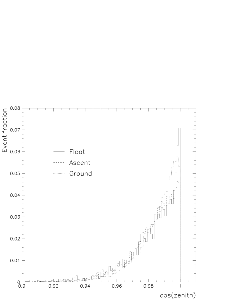
FIG. 2.: Cosine zenith angle distribution normalized to the total number of events for muons of both signs selected between 0.15 and 2 GV/$c$ at ground level (dotted histogram), during the ascent (dashed histogram) and at float (solid histogram).

FIG. 3.: The distribution of $\beta$ from the time-of-flight information as a function of rigidity for float data. The solid line is the lower limit of the muon selection. The distributions corresponding to the various particles are labelled according to the particle’s species. The figure comprises about 379000 events of which about 347000 are protons, 9000 deuterons and 6000 helium nuclei.

FIG. 4.: Total detected energy loss in the calorimeter divided by the rigidity of all particles versus rigidity for float data. A negative sign is assigned to the rigidity of negative particles. The two dense band are due to non-interacting particles. The solid line at 60 indicates the chosen upper limit used to select muons. The figure comprises about 615000 events of which about 16000 are negative particles.

FIG. 5.: Measured RICH Cherenkov angle as a function of rigidity for float data. A negative sign is assigned to the rigidity of negative particles. The figure comprises about 291000 events of which about 8000 are negative particles. The solid lines include the events accepted as muons in the RICH selection.

FIG. 6.: Geometrical factor as a function of deflection for ground and flight analysis. The lines indicate one standard deviation confidence interval.

FIG. 7.: Muon selection efficiencies for float data as a function of rigidity. The hatched area indicates one standard deviation confidence interval of the combined efficiency.

FIG. 8.: The ${\rm\mu^{+}}$ (full circles) and ${\rm\mu^{-}}$ (open circles) fluxes at float (3.9 ${\rm g/cm^{2}}$ of mean residual atmosphere) as a function of momentum.

FIG. 9.: Atmospheric growth curves for a) $\mu^{-}$ in the left panel and b) $\mu^{+}$ in the right panel. From top to bottom are the momentum ranges in GeV/$c$: 0.3–0.53 (scaled by $10^{5}$), 0.53–0.75 ($10^{4}$), 0.75–0.97 ($10^{3}$), 0.97–1.23 ($10^{2}$), 1.23–1.55 (10), 1.55–2 (1), 2–3.2 (1), 3.2–8 (1) and 8–40 (1). The $\mu^{+}$ results are shown up to 2 GeV/$c$. The solid lines are exponential fits according to equation 4.

FIG. 10.: Relative difference between the ${\rm\mu^{-}}$ fluxes obtained in this analysis and the MASS89 [23] and MASS91 [10] experiments as a function of atmospheric depth. The comparison is done for muon momenta below 1 GeV/$c$ in the upper panel (a) and between 1 and 2 GeV/$c$ in the lower panel (b). The average difference between CAPRICE94 and MASS89 is shown as a dashed line and between CAPRICE94 and MASS91 as a solid line.

FIG. 11.: Muon charge ratio as a function of atmospheric depths in two momentum intervals: (a) 0.3–1 GeV/$c$ in the upper panel and 1–2 GeV/$c$ in the lower panel (b), obtained in this analysis and from the CAPRICE98 [25], HEAT95 [26] and MASS91 experiments [10]; the latter data refer to the momentum bins 0.3–0.9 GeV/$c$ and 0.9–1.5 GeV/$c$.

FIG. 12.: Muon charge ratios as a function of momentum. In the upper panel (a) are shown the ratios obtained in this analysis at 3.9 ${\rm g/cm^{2}}$and those measured by the CAPRICE98 experiment [27] at 5.5 ${\rm g/cm^{2}}$and with the MASS91 experiment [28] at 5.7 ${\rm g/cm^{2}}$. In the lower panel (b) are shown the ratios measured at ground by this experiment (at 1000 ${\rm g/cm^{2}}$) and by the CAPRICE97 experiment (at 886 ${\rm g/cm^{2}}$) [12].

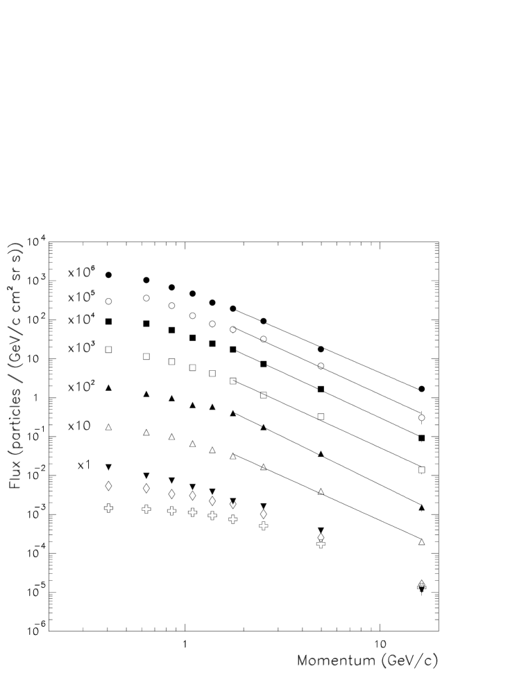
FIG. 13.: Negative muon spectra for several atmospheric depth intervals. From top to bottom are the atmospheric depth ranges in ${\rm g/cm^{2}}$: 3.3–4.6 (scaled by $10^{6}$), 7–25 (scaled by $10^{5}$), 25–70 ($10^{4}$), 70–115 ($10^{3}$), 115–165 ($10^{2}$), 165–250 (10), 250–350 (1), 350–850 (1) and 1000 (1). The solid lines are power law fits.