The tau lepton lifetime is measured with the L3 detector at LEP using the complete data taken at centre-of-mass energies around the Z pole resulting in $\tau_{\tau}\,=\,293.2\,\pm\,2.0~{}\mbox{(stat)}\,\pm\,1.5~{}\mbox{(syst)}~{}\mbox{fs}$. The comparison of this result with the muon lifetime supports lepton universality of the weak charged current at the level of six per mille. Assuming lepton universality, the value of the strong coupling constant, $\alpha_{s}$ is found to be $\alpha_{s}(m_{\tau}^{2})$ = 0.319 $\pm$ 0.015 (exp) $\pm$ 0.014 (theory).

Submitted to Phys. Lett. B

1 Introduction

In the Standard Electroweak Model [1, *GWS2, *GWS3], the couplings of the leptonic charged and neutral currents to the gauge bosons are independent of the lepton generation. Measurements of the lifetime, $\tau_{\tau}$, and the leptonic branching fractions, ${\cal{B}}(\tau\rightarrow\ell\bar{\nu}_{\ell}\nu_{\tau})$, of the tau lepton provide a test of this universality hypothesis for the charged current. The leptonic width of the tau lepton [2, *Marciano88],

$$\Gamma(\tau\rightarrow\ell\bar{\nu}_{\ell}\nu_{\tau}) \equiv \frac{{\cal{B}}(\tau\rightarrow\ell\bar{\nu}_{\ell}\nu_{\tau})}{\tau_{\tau}}$$ (1)

$$= \frac{g_{\tau}^{2}g_{\ell}^{2}}{\mbox{$m_{\mathrm{W}}$}^{4}}\frac{m_{\tau}^{5}}{96(4\pi)^{3}}(1+\epsilon_{P})\,(1+\epsilon_{rad})\,(1+\epsilon_{q^{2}}),$$ (2)

where $\ell=$e,$\mu$, depends on the coupling constants of the tau lepton and the lighter lepton to the W boson, $g_{\tau}$ and $g_{\ell}$, respectively. Here $m_{\tau}$ and $m_{\mathrm{W}}$ are the masses of the tau lepton and the W boson. The quantities $\epsilon_{P}$, $\epsilon_{rad}$ and $\epsilon_{q^{2}}$ are small corrections resulting from phase-space, radiation and the W propagator, respectively. For the decay of the muon, $\mu\rightarrow\mathrm{e}\bar{\nu}_{\mathrm{e}}\nu_{\mu}$, the same formula applies, with the muon mass and coupling, $m_{\mu}$ and $g_{\mu}$, replacing those of the tau. The comparison of the tau lifetime and leptonic branching fractions with the muon lifetime gives a direct measurement of the ratios $g_{\tau}/g_{\mathrm{e}}$ and $g_{\tau}/g_{\mu}$.

Tau decays into hadrons are sensitive to the strong coupling constant, $\alpha_{s}$, at the tau mass scale. Assuming universal coupling constants of the different lepton species to the W boson, the ratio of the hadronic width to the leptonic width, $R_{\tau}$, can be expressed as:

$$R_{\tau}=\left(\frac{m_{\mu}}{m_{\tau}}\right)^{5}\frac{\tau_{\mu}}{\tau_{\tau}}-C,$$ (3)

where $C=1.9726$ contains the same corrections mentioned above.

$R_{\tau}$ is calculated in perturbative QCD  [3, 4, 5]:

$$R_{\tau}=3(|V_{\mathrm{ud}}|^{2}+|V_{\mathrm{us}}|^{2})S_{EW}(1+\frac{\alpha_{s}}{\pi}\,+\,5.2023(\frac{\alpha_{s}}{\pi})^{2}\,+\,26.366(\frac{\alpha_{s}}{\pi})^{3}\,+\,(78+d_{3})(\frac{\alpha_{s}}{\pi})^{4}\,+\,\delta_{NP}).$$ (4)

The quantities $|V_{\mathrm{ud}}|$ and $|V_{\mathrm{us}}|$ are elements of the Cabibbo-Kobayashi-Maskawa (CKM) quark mixing matrix [6, *ckm2], $S_{EW}$ [7] and $\delta_{NP}$ [4, 8] describe electroweak radiative corrections and non-perturbative QCD contributions, respectively. The quantity $d_{3}$ is estimated as $d_{3}$ = 27.5 [5]. The perturbative theoretical uncertainty is taken to be $d_{3}$ = 27.5$\pm$27.5.

This paper presents a measurement of the tau lepton lifetime with the L3 detector at LEP, using data taken in 1995 at the $\Zo$ pole. Furthermore, data from 1994 are re-analysed using an improved calibration and alignment of the central tracker. The lifetime is measured from the decay length in three-prong tau decays and from the impact parameter of one-prong tau decays. The results are combined with our previously published analyses on data collected from 1990 to 1993 [9, *mblife1]. Previous measurements of the tau lepton lifetime have been reported by other experiments [10].

2 L3 Detector

The L3 detector is described in Ref. [11]. This measurement is based primarily on the information obtained from the central tracking system, which is composed of a Silicon Microvertex Detector (SMD) [12, *smd_09], a Time Expansion Chamber (TEC) and a Z-chamber. The SMD is made of two concentric layers of double-sided silicon detectors, placed at about 6 and 8 cm from the beam line. Each layer provides a two-dimensional position measurement, with a resolution of $7~{}\mbox{and}~{}14~{}\mu\mbox{m}$ for normally incident tracks, in the directions perpendicular and parallel to the beam direction, denoted as $(x,y)$ and $z$ coordinates, respectively. The TEC consists of two coaxial cylindrical drift chambers with 12 inner and 24 outer sectors. The sensitive region is between 10 and 45 cm in the radial direction, with 62 anode wires having a spatial resolution of approximately $50~{}\mu\mbox{m}$ in the plane perpendicular to the beam axis. The Z-chamber, which is situated just outside the TEC, provides a coordinate measurement along the beam axis direction.

3 Event Sample

For this measurement data collected in 1994 and 1995 are used, which correspond to an integrated luminosity of 49 pb^-1 and 31 pb^-1, respectively.

For efficiency and background estimates, Monte Carlo events are generated using the programs KORALZ [13] for $\rm e^{+}e^{-}\rightarrow\mu^{+}\mu^{-}(\gamma)$ and e⁺e${}^{-}\rightarrow\tau^{+}\tau^{-}(\gamma)$, BHAGENE [14, *bhagene2] for $\rm e^{+}e^{-}\rightarrow e^{+}e^{-}(\gamma)$, DIAG36 [15] for $\rm e^{+}e^{-}\rightarrow e^{+}e^{-}f\bar{f}$, where $\rm f\bar{f}$ is $\rm e^{+}e^{-}$, $\mu^{+}\mu^{-}$, $\tau^{+}\tau^{-}$ or $\rm q\bar{q}$, and JETSET [16] for $\ee\ra\mathrm{q}\bar{\mathrm{q}}(\gamma)$. The Monte Carlo events are passed through a full detector simulation based on the GEANT program [17], which takes into account the effects of energy loss, multiple scattering, showering and small time dependent detector inefficiencies. These events are reconstructed with the same program used for the data. The number of Monte Carlo events in each process is about ten times larger than the corresponding data sample.

Tau lepton pairs originating from $\Zo$ decays are characterised by two low multiplicity, highly collimated jets in the detector. The selection of e⁺e${}^{-}\rightarrow\tau^{+}\tau^{-}(\gamma)$ events is described in detail in Ref. [18]; here only a general outline is given. In order to have high-quality reconstruction of the tracks, events are accepted within a fiducial volume defined by $|\cos\theta_{t}|<0.72$, where the polar angle $\theta_{t}$ is given by the thrust axis of the event with respect to the electron beam direction. The events must have at least two jets, and the number of tracks in each jet must be less than four. The background from $\mathrm{e^{+}e^{-}}\rightarrow\mathrm{e^{+}e^{-}}~{}(\gamma)$ events is reduced by requiring the total energy deposited in the electromagnetic calorimeter to be less than $75\%$ of the centre-of-mass energy. To reduce background from $\mathrm{e^{+}e^{-}}\rightarrow\mu^{+}\mu^{-}~{}(\gamma)$ the sum of the absolute momenta measured in the muon spectrometer must be less than $70\%$ of the centre-of-mass energy. If muons are not reconstructed in the muon chambers they are identified by an energy deposit in the calorimeters which is characteristic of a minimum ionising particle. If this is the case for one jet, the opposite jet is required to exhibit a hadronic signature. This rejects dimuon as well as cosmic-ray events. The cosmic-ray background is further reduced by requiring a scintillation counter hit within 5 ns of the beam crossing. In addition, the distance of closest approach to the interaction point measured by the muon chambers must be less than two standard deviations of the resolution.

Following this procedure, $29679$ and $13294$ events are selected from the data collected in 1994 and 1995, respectively. The selection efficiency in the fiducial volume is estimated to be 76%. The purity of the tau pair sample is 98%.

4 Tracking

For this measurement a high quality of the track reconstruction is essential. A prerequisite is the control of the alignment between SMD and TEC and the drift time to drift distance calibration for the TEC. These calibrations, alignments and the estimation of resolution functions are performed with a clean sample of Bhabha and dimuon events, where tracks are known to originate from a common vertex. Particular effort is invested in the individual alignment of each sensor of the SMD and in the calibration of the boundaries of the TEC sectors. The procedure is described in detail in Ref. [19]. The performance of the track reconstruction is estimated from the distance between the two tracks at the vertex projected into the $(x,y)$ plane. This quantity, called miss distance, is independent of the size and position of the $\mathrm{e}^{+}\mathrm{e}^{-}$ interaction region. The distributions of miss distance for Bhabha and dimuon events collected during 1994 and 1995 are shown in Figure 1. A Gaussian function is fitted to both distributions, from which an intrinsic resolution $\sigma_{\mbox{\scriptsize int}}=33~{}\mu\mbox{m}$ and $31~{}\mu\mbox{m}$ is estimated for 1994 and 1995, respectively.

To guarantee good tracks for the analysis, the following cuts are made:

• Number of hits in the TEC $\geq 30$. This ensures a good curvature measurement.

• Number of SMD hits in the $(x,y)$ plane $\geq 1$. This criterion selects tracks for which the error in the extrapolation to the vertex is well described by $\sigma_{\mbox{\scriptsize int}}$.

• Transverse momentum, $|p_{t}|\geq 500~{}\mbox{MeV}$. Tracks with lower momenta have a larger uncertainty in the extrapolation to the vertex due to multiple Coulomb scattering in the SMD.

• Probability, $P(\chi^{2})$, of the track fit larger than 1%. This requirement rejects bad fits.

5 Decay Length Method

For three-prong tau decays, the decay vertex of the tau is reconstructed and its distance to the centre of the interaction region is measured. The decay vertex is found from a minimisation with respect to the vertex coordinates $(x_{v},\,y_{v})$ of the following $\chi^{2}$:

$$\chi^{2}\,=\,\sum_{i=1}^{N_{\mbox{\scriptsize track}}}\left(\frac{\delta_{i}(x_{v},\,y_{v})}{\sigma_{\delta_{i}}}\right)^{2}.$$ (5)

In this equation, $\delta_{i}$ is the distance of closest approach of a track to the decay vertex coordinates. The error, $\sigma_{\delta_{i}}$, is the quadratic sum of the intrinsic resolution, $\sigma_{\mbox{\scriptsize int}}$, and the error due to multiple Coulomb scattering, $\sigma_{\mbox{\scriptsize ms}}(p)$. Figure 2 shows the distribution of the confidence level, $P(\chi^{2})$, of the fit. Decay vertices with $P(\chi^{2})<1\%$ contain in most cases tracks with wrongly matched SMD hits and are rejected. The remaining distribution is flat, indicating a good description of the errors.

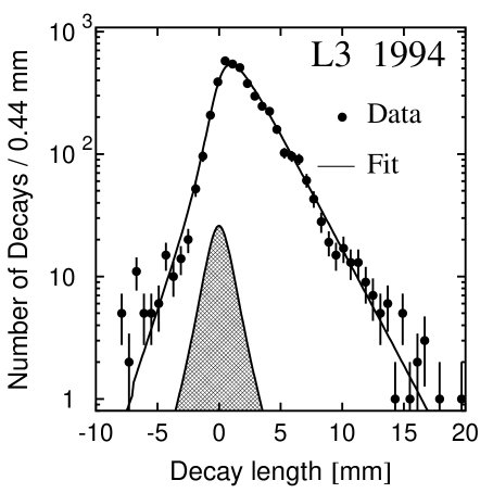
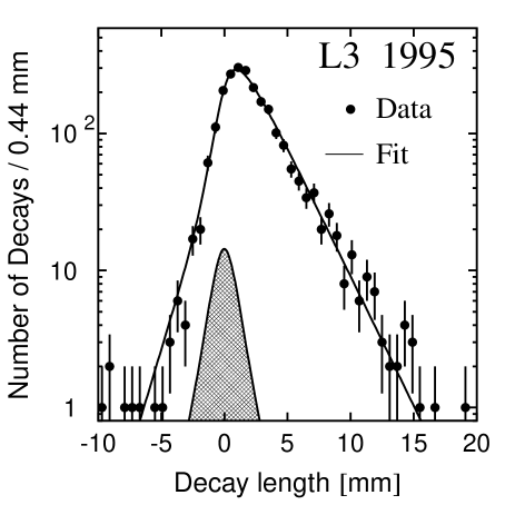
Figure 3: Decay length distributions from 1994 (left) and 1995 (right); Three-prong tau decays are shown in linear scale (upper) and logarithmic scale (lower). The hatched areas represent the distributions of background events carrying no lifetime information.

Figure 3 shows the decay length distribution for the data collected in 1994 and 1995. Only decay length values in the range $[-10,\,20]~{}\mbox{mm}$ with an error better than 5 mm are accepted for the lifetime determination. The number of selected decays is $4306$ and $2314$ for 1994 and 1995 data, respectively.

To obtain the average decay length, an unbinned maximum likelihood fit is applied to the observed decay length distribution. The likelihood function is calculated from a convolution of an exponential $E$, describing the tau decay time using the average decay length $\langle L\rangle$ as a parameter, with a Gaussian resolution function $R$. The likelihood function is written as:

$${\cal{L}}\,=\,\prod_{i=1}^{N_{3p}}(1-f_{B})\cdot E\otimes R+f_{B}\cdot B.$$ (6)

In this equation the product runs over the accepted three-prong tau decays $N_{3p}$. The second term on the right hand side has been added to take into account background carrying no $\tau$ lifetime information. The background fraction, $f_{B}$, is estimated from Monte Carlo and fixed in the fit. The likelihood function $B$ is evaluated from the convolution of a Dirac delta function with the experimental resolution function.

The fit minimises $-\log\cal L$. Average decay lengths of $\langle L\rangle\,=\,(\,2.245\,\pm\,0.037\,)~{}\mbox{mm}$ and $\langle L\rangle\,=\,(\,2.265\,\pm\,0.051\,)~{}\mbox{mm}$ are determined for data from 1994 and 1995, respectively. The results of the fit are represented by the solid lines in Figure 3.

The tau lifetime and average decay length are related through the following expression:

$$\tau_{\tau}\,=\,\frac{\langle L\rangle}{\beta\,\gamma\,c}.$$ (7)

Using this equation and taking into account the effects of radiation, lifetimes of $\tau_{\tau}\,=\,292.5\,\pm\,4.9~{}\mbox{fs}$ and $\tau_{\tau}\,=\,295.2\,\pm\,6.6~{}\mbox{fs}$ are obtained for the two data sets, where the errors are statistical only.

In order to check the decay length method, the analysis is repeated on a sample of Monte Carlo events. The difference between the input tau lifetime and the result of the fit is assigned as a systematic error due to the method. Systematic effects due to the non-ideal description of the resolution function are estimated from a one $\sigma$ variation of its parameters. The deviation of the SMD radius from its nominal value is measured using Bhabha and dimuon events by minimising the track coordinate residuals from overlapping silicon sensors. Deviations of $(-5\pm 5)~{}\mu\mbox{m}$ and $(-3\pm 5)~{}\mu\mbox{m}$ are found in the data of 1994 and 1995, respectively. These results are compatible with zero, and their uncertainties are translated into a systematic error on the lifetime. Uncertainties in the fraction of background events carrying no lifetime information are estimated from a $\pm\,50\%$ variation of the fraction. Finally, the systematic error due to the fit range is estimated from the combined data by a 10% variation of their lower and upper bounds. This error also includes the effect of a variation of the cut on $P(\chi^{2})$ between 0.1 and 1.5%. Table 1 summarises the systematic errors for the decay length method.

The lifetime measurements from the $6620$ three-prong decays from 1994 and 1995 are combined. The systematic error due to the resolution function description is taken to be uncorrelated; for the other errors a 100% correlation is assumed. The result is $\tau_{\tau}\,=\,292.9\,\pm\,3.9~{}\mbox{(stat)}\,\pm\,1.9~{}\mbox{(syst)}~{}\mbox{fs}.$

6 Impact Parameter Method

A second measurement of the tau lifetime is obtained from the impact parameter in the plane perpendicular to the beam axis for one-prong tau decays. The impact parameter is the distance of closest approach, $\delta$, of the track to the tau lepton production point, which is estimated by the beam position. In order to be sensitive to the lifetime, a sign is given to the impact parameter, according to the position of the intersection between the track and the tau direction of flight with respect to the beam position. The uncertainty on the impact parameter, $\sigma_{\mbox{\scriptsize ip}}$, is described as the quadratic sum of the intrinsic detector resolution, $\sigma_{\mbox{\scriptsize int}}$, the size of the interaction region, $(\sigma_{x},\,\sigma_{y})$, and a momentum dependent multiple Coulomb scattering contribution, $\sigma_{\mbox{\scriptsize ms}}(p)$,

$$\sigma_{\mbox{\scriptsize ip}}^{2}\,=\,\sigma_{\mbox{\scriptsize int}}^{2}\,+\,\sigma_{x}^{2}\sin^{2}\phi\,+\,\sigma_{y}^{2}\cos^{2}\phi\,+\,\sigma_{\mbox{\scriptsize ms}}^{2}(p),$$ (8)

where $\phi$ is the azimuthal angle in the plane perpendicular to the beam axis. The average values for the interaction region size are determined from Bhabha and dimuon data and listed in Table 2.

In contrast to the decay length method a more complicated function for the description of the tau decay is expected here, since for a one-prong tau decay the decay vertex is a priori not known. From a Monte Carlo study of the impact parameter distribution at generator level it is found that this function can be described in terms of three exponentials for positive and three exponentials for negative impact parameter values

$$U(\delta)\,=\,(1-W)\sum_{i=1}^{3}\frac{f_{i}^{+}}{\lambda_{i}^{+}}e^{-\frac{\delta}{\lambda_{i}^{+}}}\,+\,W\sum_{i=1}^{3}\frac{f_{i}^{-}}{\lambda_{i}^{-}}e^{\frac{\delta}{\lambda_{i}^{-}}}.$$ (9)

In this equation, $W$ represents the fraction of negative impact parameter values, which originate from an imperfect reconstruction of the tau flight direction. The slopes of the exponentials, $\lambda_{i}$, contain the lifetime dependence of the distribution.

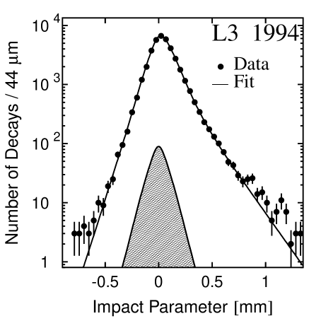
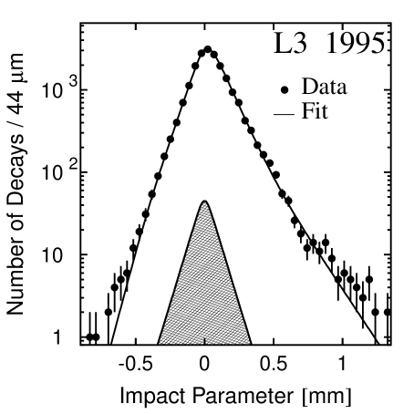
Figure 4: Impact parameter distributions from 1994 (left) and 1995 (right); One-prong tau decays are shown in linear scale (upper) and logarithmic scale (lower). The hatched areas represent the distributions of background events which carry no lifetime information.

As for the decay length method, the lifetime is extracted from an unbinned maximum likelihood fit to the observed distribution. The likelihood is now determined from the convolution of a double Gaussian resolution function, which is obtained from Bhabha and dimuon samples, with the function of Eqn.(9). The fit also accounts for background carrying no lifetime information. Figure 4 shows the impact parameter distributions from tau decays collected in 1994 and 1995. Impact parameters with a value in the range $[-0.9,\,1.35]~{}\mbox{mm}$ and an impact parameter error of less than $250~{}\mu\mbox{m}$ are accepted for the measurement. The fit yields a tau lifetime of $\tau_{\tau}\,=\,292.7\,\pm\,3.3\,\mbox{fs}$ and $\tau_{\tau}\,=\,295.0\,\pm\,4.9~{}\mbox{fs}$ for the two data samples. The errors are statistical only.

The method is checked on a Monte Carlo sample, from which the lifetime is determined in the same way as for the data. The difference between the input tau lifetime and the result of the fit is assigned as a systematic error due to the method. Systematic effects due to the uncertainty of the resolution function are estimated from a variation of its parameters according to their errors, with correlations taken into account. The beam spot size is varied according to its statistical errors. The change in the central value is assigned as a systematic uncertainty. The effect of the average SMD radial position uncertainty is treated in the same way as in the decay length analysis. The systematic effect due to the knowledge of the function $U(\delta)$ is evaluated by taking into account its statistical uncertainty and its dependence on the tau lifetime in the range from 250 to 350 fs. The uncertainty arising from the fraction of background events is estimated from a $\pm\,50\%$ variation of this fraction. The systematic error induced by the choice of the fit ranges is estimated from the combined data sample by a 10% variation of their bounds. Table 3 summarises the systematic errors for the impact parameter method.

The lifetime measurements from the $58656$ one-prong decays from 1994 and 1995 are combined. The systematic error due to the resolution function is taken to be uncorrelated. For the other errors a 100% correlation has been assumed. The result is $\tau_{\tau}\,=\,292.8\,\pm\,2.7~{}\mbox{(stat)}\,\pm\,2.0~{}\mbox{(syst)}~{}\mbox{fs}.$

7 Discussion

The combination of the results obtained by the two methods with our previous ones [9, *mblife1] yields

$$\tau_{\tau}\,=\,293.2\,\pm\,2.0~{}\mbox{(stat)}\,\pm\,1.5~{}\mbox{(syst)}~{}\mbox{fs}.$$ (10)

Correlations within the systematic errors are taken into account. This result supersedes all previous results [9, *mblife1, 18]. This value is in good agreement with the current world average [20].

The measurements of the branching fractions, ${\cal{B}}(\tau\rightarrow\mathrm{e}\bar{\nu}_{\mathrm{e}}\nu_{\tau})=(17.806~{}\pm~{}0.129)\%$ and ${\cal{B}}(\tau\rightarrow\mu\bar{\nu}_{\mu}\nu_{\tau})=(17.341~{}\pm~{}0.129)\%$ [21] together with this lifetime measurement and the muon lifetime [20] yield $g_{\tau}/g_{\mathrm{e}}=0.996~{}\pm~{}0.006$ and $g_{\tau}/g_{\mu}=0.996~{}\pm~{}0.006$ supporting the universality hypothesis.

From the tau lifetime, the tau mass, the muon mass and muon lifetime, $R_{\tau}$ is found to be $R_{\tau}=3.595~{}\pm~{}0.048$. This corresponds to

$$\alpha_{s}(m_{\tau}^{2})=0.319~{}\pm~{}0.015~{}\mbox{(exp)}~{}\pm~{}0.014~{}\mbox{(theory)}.$$ (11)

The first error is due to the errors of the tau lifetime and the CKM matrix elements [20]. The second error is the quadratic sum of the uncertainties resulting from the renormalisation scale, the term fourth order in $\alpha_{s}$, the electroweak corrections $S_{EW}$, and the non-perturbative correction, $\delta_{NP}$. The renormalisation scale uncertainty is estimated following Ref. [22] by a variation between 0.4 $\leq m_{\tau}^{2}/\mu^{2}\leq$ 2.0 and is the dominant contribution to the error. Other contributions to the theory error as discussed in Ref. [23] are not considered. This result is in good agreement with other measurements of $\alpha_{s}$ at the tau mass [24, 20]. The value of $\alpha_{s}(m_{\tau}^{2})$ is extrapolated to the $\Zo$ mass using the renormalisation group equation [25] with the four loop calculation of the QCD $\beta$-functions [26]. The result, $\alpha_{s}(\mbox{$m_{\mathrm{Z}}$}^{2})$ = 0.1185 $\pm$ 0.0019 (exp) $\pm$ 0.0017 (theory), is in good agreement with the current world average value [20].

The L3 Collaboration:

M.Acciarri,²⁶ P.Achard,¹⁹ O.Adriani,¹⁶ M.Aguilar-Benitez,²⁵ J.Alcaraz,²⁵ G.Alemanni,²² J.Allaby,¹⁷ A.Aloisio,²⁸ M.G.Alviggi,²⁸ G.Ambrosi,¹⁹ H.Anderhub,⁴⁸ V.P.Andreev,^6,36 T.Angelescu,¹² F.Anselmo,⁹ A.Arefiev,²⁷ T.Azemoon,³ T.Aziz,¹⁰ P.Bagnaia,³⁵ A.Bajo,²⁵ L.Baksay,⁴³ A.Balandras,⁴ S.Banerjee,¹⁰ Sw.Banerjee,¹⁰ A.Barczyk,^48,46 R.Barillère,¹⁷ L.Barone,³⁵ P.Bartalini,²² M.Basile,⁹ R.Battiston,³² A.Bay,²² F.Becattini,¹⁶ U.Becker,¹⁴ F.Behner,⁴⁸ L.Bellucci,¹⁶ R.Berbeco,³ J.Berdugo,²⁵ P.Berges,¹⁴ B.Bertucci,³² B.L.Betev,⁴⁸ S.Bhattacharya,¹⁰ M.Biasini,³² A.Biland,⁴⁸ J.J.Blaising,⁴ S.C.Blyth,³³ G.J.Bobbink,² A.Böhm,¹ L.Boldizsar,¹³ B.Borgia,³⁵ D.Bourilkov,⁴⁸ M.Bourquin,¹⁹ S.Braccini,¹⁹ J.G.Branson,³⁹ V.Brigljevic,⁴⁸ F.Brochu,⁴ A.Buffini,¹⁶ A.Buijs,⁴⁴ J.D.Burger,¹⁴ W.J.Burger,³² X.D.Cai,¹⁴ M.Campanelli,⁴⁸ M.Capell,¹⁴ G.Cara Romeo,⁹ G.Carlino,²⁸ A.M.Cartacci,¹⁶ J.Casaus,²⁵ G.Castellini,¹⁶ F.Cavallari,³⁵ N.Cavallo,³⁷ C.Cecchi,³² M.Cerrada,²⁵ F.Cesaroni,²³ M.Chamizo,¹⁹ Y.H.Chang,⁵⁰ U.K.Chaturvedi,¹⁸ M.Chemarin,²⁴ A.Chen,⁵⁰ G.Chen,⁷ G.M.Chen,⁷ H.F.Chen,²⁰ H.S.Chen,⁷ G.Chiefari,²⁸ L.Cifarelli,³⁸ F.Cindolo,⁹ C.Civinini,¹⁶ I.Clare,¹⁴ R.Clare,¹⁴ G.Coignet,⁴ A.P.Colijn,² N.Colino,²⁵ S.Costantini,⁵ F.Cotorobai,¹² B.Cozzoni,⁹ B.de la Cruz,²⁵ A.Csilling,¹³ S.Cucciarelli,³² T.S.Dai,¹⁴ J.A.van Dalen,³⁰ R.D’Alessandro,¹⁶ R.de Asmundis,²⁸ P.Déglon,¹⁹ A.Degré,⁴ K.Deiters,⁴⁶ D.della Volpe,²⁸ P.Denes,³⁴ F.DeNotaristefani,³⁵ A.De Salvo,⁴⁸ M.Diemoz,³⁵ D.van Dierendonck,² F.Di Lodovico,⁴⁸ C.Dionisi,³⁵ M.Dittmar,⁴⁸ A.Dominguez,³⁹ A.Doria,²⁸ M.T.Dova,^18,♯ D.Duchesneau,⁴ D.Dufournaud,⁴ P.Duinker,² I.Duran,⁴⁰ H.El Mamouni,²⁴ A.Engler,³³ F.J.Eppling,¹⁴ F.C.Erné,² P.Extermann,¹⁹ M.Fabre,⁴⁶ R.Faccini,³⁵ M.A.Falagan,²⁵ S.Falciano,^35,17 A.Favara,¹⁷ J.Fay,²⁴ O.Fedin,³⁶ M.Felcini,⁴⁸ T.Ferguson,³³ F.Ferroni,³⁵ H.Fesefeldt,¹ E.Fiandrini,³² J.H.Field,¹⁹ F.Filthaut,¹⁷ P.H.Fisher,¹⁴ I.Fisk,³⁹ G.Forconi,¹⁴ L.Fredj,¹⁹ K.Freudenreich,⁴⁸ C.Furetta,²⁶ Yu.Galaktionov,^27,14 S.N.Ganguli,¹⁰ P.Garcia-Abia,⁵ M.Gataullin,³¹ S.S.Gau,¹¹ S.Gentile,^35,17 N.Gheordanescu,¹² S.Giagu,³⁵ Z.F.Gong,²⁰ G.Grenier,²⁴ O.Grimm,⁴⁸ M.W.Gruenewald,⁸ M.Guida,³⁸ R.van Gulik,² V.K.Gupta,³⁴ A.Gurtu,¹⁰ L.J.Gutay,⁴⁵ D.Haas,⁵ A.Hasan,²⁹ D.Hatzifotiadou,⁹ T.Hebbeker,⁸ A.Hervé,¹⁷ P.Hidas,¹³ J.Hirschfelder,³³ H.Hofer,⁴⁸ G. Holzner,⁴⁸ H.Hoorani,³³ S.R.Hou,⁵⁰ Y.Hu,³⁰ I.Iashvili,⁴⁷ B.N.Jin,⁷ L.W.Jones,³ P.de Jong,² I.Josa-Mutuberría,²⁵ R.A.Khan,¹⁸ M.Kaur,^18,♢ M.N.Kienzle-Focacci,¹⁹ D.Kim,³⁵ J.K.Kim,⁴² J.Kirkby,¹⁷ D.Kiss,¹³ W.Kittel,³⁰ A.Klimentov,^14,27 A.C.König,³⁰ A.Kopp,⁴⁷ V.Koutsenko,^14,27 M.Kräber,⁴⁸ R.W.Kraemer,³³ W.Krenz,¹ A.Krüger,⁴⁷ A.Kunin,^14,27 P.Ladron de Guevara,²⁵ I.Laktineh,²⁴ G.Landi,¹⁶ K.Lassila-Perini,⁴⁸ M.Lebeau,¹⁷ A.Lebedev,¹⁴ P.Lebrun,²⁴ P.Lecomte,⁴⁸ P.Lecoq,¹⁷ P.Le Coultre,⁴⁸ H.J.Lee,⁸ J.M.Le Goff,¹⁷ R.Leiste,⁴⁷ E.Leonardi,³⁵ P.Levtchenko,³⁶ C.Li,²⁰ S.Likhoded,⁴⁷ C.H.Lin,⁵⁰ W.T.Lin,⁵⁰ F.L.Linde,² L.Lista,²⁸ Z.A.Liu,⁷ W.Lohmann,⁴⁷ E.Longo,³⁵ Y.S.Lu,⁷ K.Lübelsmeyer,¹ C.Luci,^17,35 D.Luckey,¹⁴ L.Lugnier,²⁴ L.Luminari,³⁵ W.Lustermann,⁴⁸ W.G.Ma,²⁰ M.Maity,¹⁰ L.Malgeri,¹⁷ A.Malinin,¹⁷ C.Maña,²⁵ D.Mangeol,³⁰ J.Mans,³⁴ P.Marchesini,⁴⁸ G.Marian,¹⁵ J.P.Martin,²⁴ F.Marzano,³⁵ G.G.G.Massaro,² K.Mazumdar,¹⁰ R.R.McNeil,⁶ S.Mele,¹⁷ L.Merola,²⁸ M.Meschini,¹⁶ W.J.Metzger,³⁰ M.von der Mey,¹ A.Mihul,¹² H.Milcent,¹⁷ G.Mirabelli,³⁵ J.Mnich,¹⁷ G.B.Mohanty,¹⁰ P.Molnar,⁸ B.Monteleoni,^16,† R.Moore,³ T.Moulik,¹⁰ G.S.Muanza,²⁴ F.Muheim,¹⁹ A.J.M.Muijs,² M.Musy,³⁵ M.Napolitano,²⁸ F.Nessi-Tedaldi,⁴⁸ H.Newman,³¹ T.Niessen,¹ A.Nisati,³⁵ H.Nowak,⁴⁷ G.Organtini,³⁵ A.Oulianov,²⁷ C.Palomares,²⁵ D.Pandoulas,¹ S.Paoletti,^35,17 P.Paolucci,²⁸ R.Paramatti,³⁵ H.K.Park,³³ I.H.Park,⁴² G.Pascale,³⁵ G.Passaleva,¹⁷ S.Patricelli,²⁸ T.Paul,¹¹ M.Pauluzzi,³² C.Paus,¹⁷ F.Pauss,⁴⁸ M.Pedace,³⁵ S.Pensotti,²⁶ D.Perret-Gallix,⁴ B.Petersen,³⁰ D.Piccolo,²⁸ F.Pierella,⁹ M.Pieri,¹⁶ P.A.Piroué,³⁴ E.Pistolesi,²⁶ V.Plyaskin,²⁷ M.Pohl,¹⁹ V.Pojidaev,^27,16 H.Postema,¹⁴ J.Pothier,¹⁷ N.Produit,¹⁹ D.O.Prokofiev,⁴⁵ D.Prokofiev,³⁶ J.Quartieri,³⁸ G.Rahal-Callot,^48,17 M.A.Rahaman,¹⁰ P.Raics,¹⁵ N.Raja,¹⁰ R.Ramelli,⁴⁸ P.G.Rancoita,²⁶ A.Raspereza,⁴⁷ G.Raven,³⁹ P.Razis,²⁹D.Ren,⁴⁸ M.Rescigno,³⁵ S.Reucroft,¹¹ T.van Rhee,⁴⁴ S.Riemann,⁴⁷ K.Riles,³ A.Robohm,⁴⁸ J.Rodin,⁴³ B.P.Roe,³ L.Romero,²⁵ A.Rosca,⁸ S.Rosier-Lees,⁴ J.A.Rubio,¹⁷ D.Ruschmeier,⁸ H.Rykaczewski,⁴⁸ S.Saremi,⁶ S.Sarkar,³⁵ J.Salicio,¹⁷ E.Sanchez,¹⁷ M.P.Sanders,³⁰ M.E.Sarakinos,²¹ C.Schäfer,¹⁷ V.Schegelsky,³⁶ S.Schmidt-Kaerst,¹ D.Schmitz,¹ H.Schopper,⁴⁹ D.J.Schotanus,³⁰ G.Schwering,¹ C.Sciacca,²⁸ D.Sciarrino,¹⁹ A.Seganti,⁹ L.Servoli,³² S.Shevchenko,³¹ N.Shivarov,⁴¹ V.Shoutko,²⁷ E.Shumilov,²⁷ A.Shvorob,³¹ T.Siedenburg,¹ D.Son,⁴² B.Smith,³³ P.Spillantini,¹⁶ M.Steuer,¹⁴ D.P.Stickland,³⁴ A.Stone,⁶ B.Stoyanov,⁴¹ A.Straessner,¹ K.Sudhakar,¹⁰ G.Sultanov,¹⁸ L.Z.Sun,²⁰ H.Suter,⁴⁸ J.D.Swain,¹⁸ Z.Szillasi,^43,¶ T.Sztaricskai,^43,¶ X.W.Tang,⁷ L.Tauscher,⁵ L.Taylor,¹¹ B.Tellili,²⁴ C.Timmermans,³⁰ Samuel C.C.Ting,¹⁴ S.M.Ting,¹⁴ S.C.Tonwar,¹⁰ J.Tóth,¹³ C.Tully,¹⁷ K.L.Tung,⁷Y.Uchida,¹⁴ J.Ulbricht,⁴⁸ E.Valente,³⁵ G.Vesztergombi,¹³ I.Vetlitsky,²⁷ D.Vicinanza,³⁸ G.Viertel,⁴⁸ S.Villa,¹¹ M.Vivargent,⁴ S.Vlachos,⁵ I.Vodopianov,³⁶ H.Vogel,³³ H.Vogt,⁴⁷ I.Vorobiev,²⁷ A.A.Vorobyov,³⁶ A.Vorvolakos,²⁹ M.Wadhwa,⁵ W.Wallraff,¹ M.Wang,¹⁴ X.L.Wang,²⁰ Z.M.Wang,²⁰ A.Weber,¹ M.Weber,¹ P.Wienemann,¹ H.Wilkens,³⁰ S.X.Wu,¹⁴ S.Wynhoff,¹⁷ L.Xia,³¹ Z.Z.Xu,²⁰ J.Yamamoto,³ B.Z.Yang,²⁰ C.G.Yang,⁷ H.J.Yang,⁷ M.Yang,⁷ J.B.Ye,²⁰ S.C.Yeh,⁵¹ An.Zalite,³⁶ Yu.Zalite,³⁶ Z.P.Zhang,²⁰ G.Y.Zhu,⁷ R.Y.Zhu,³¹ A.Zichichi,^9,17,18 F.Ziegler,⁴⁷ G.Zilizi,^43,¶ M.Zöller.¹

• I. Physikalisches Institut, RWTH, D-52056 Aachen, FRG^§
  III. Physikalisches Institut, RWTH, D-52056 Aachen, FRG^§

• National Institute for High Energy Physics, NIKHEF, and University of Amsterdam, NL-1009 DB Amsterdam, The Netherlands

• University of Michigan, Ann Arbor, MI 48109, USA

• Laboratoire d’Annecy-le-Vieux de Physique des Particules, LAPP,IN2P3-CNRS, BP 110, F-74941 Annecy-le-Vieux CEDEX, France

• Institute of Physics, University of Basel, CH-4056 Basel, Switzerland

• Louisiana State University, Baton Rouge, LA 70803, USA

• Institute of High Energy Physics, IHEP, 100039 Beijing, China^△

• Humboldt University, D-10099 Berlin, FRG^§

• University of Bologna and INFN-Sezione di Bologna, I-40126 Bologna, Italy

• Tata Institute of Fundamental Research, Bombay 400 005, India

• Northeastern University, Boston, MA 02115, USA

• Institute of Atomic Physics and University of Bucharest, R-76900 Bucharest, Romania

• Central Research Institute for Physics of the Hungarian Academy of Sciences, H-1525 Budapest 114, Hungary^‡

• Massachusetts Institute of Technology, Cambridge, MA 02139, USA

• KLTE-ATOMKI, H-4010 Debrecen, Hungary^¶

• INFN Sezione di Firenze and University of Florence, I-50125 Florence, Italy

• European Laboratory for Particle Physics, CERN, CH-1211 Geneva 23, Switzerland

• World Laboratory, FBLJA Project, CH-1211 Geneva 23, Switzerland

• University of Geneva, CH-1211 Geneva 4, Switzerland

• Chinese University of Science and Technology, USTC, Hefei, Anhui 230 029, China^△

• SEFT, Research Institute for High Energy Physics, P.O. Box 9, SF-00014 Helsinki, Finland

• University of Lausanne, CH-1015 Lausanne, Switzerland

• INFN-Sezione di Lecce and Universitá Degli Studi di Lecce, I-73100 Lecce, Italy

• Institut de Physique Nucléaire de Lyon, IN2P3-CNRS,Université Claude Bernard, F-69622 Villeurbanne, France

• Centro de Investigaciones Energéticas, Medioambientales y Tecnologícas, CIEMAT, E-28040 Madrid, Spain${\flat}$

• INFN-Sezione di Milano, I-20133 Milan, Italy

• Institute of Theoretical and Experimental Physics, ITEP, Moscow, Russia

• INFN-Sezione di Napoli and University of Naples, I-80125 Naples, Italy

• Department of Natural Sciences, University of Cyprus, Nicosia, Cyprus

• University of Nijmegen and NIKHEF, NL-6525 ED Nijmegen, The Netherlands

• California Institute of Technology, Pasadena, CA 91125, USA

• INFN-Sezione di Perugia and Universitá Degli Studi di Perugia, I-06100 Perugia, Italy

• Carnegie Mellon University, Pittsburgh, PA 15213, USA

• Princeton University, Princeton, NJ 08544, USA

• INFN-Sezione di Roma and University of Rome, “La Sapienza”, I-00185 Rome, Italy

• Nuclear Physics Institute, St. Petersburg, Russia

• INFN-Sezione di Napoli and University of Potenza, I-85100 Potenza, Italy

• University and INFN, Salerno, I-84100 Salerno, Italy

• University of California, San Diego, CA 92093, USA

• Dept. de Fisica de Particulas Elementales, Univ. de Santiago, E-15706 Santiago de Compostela, Spain

• Bulgarian Academy of Sciences, Central Lab. of Mechatronics and Instrumentation, BU-1113 Sofia, Bulgaria

• Laboratory of High Energy Physics, Kyungpook National University, 702-701 Taegu, Republic of Korea

• University of Alabama, Tuscaloosa, AL 35486, USA

• Utrecht University and NIKHEF, NL-3584 CB Utrecht, The Netherlands

• Purdue University, West Lafayette, IN 47907, USA

• Paul Scherrer Institut, PSI, CH-5232 Villigen, Switzerland

• DESY, D-15738 Zeuthen, FRG

• Eidgenössische Technische Hochschule, ETH Zürich, CH-8093 Zürich, Switzerland

• University of Hamburg, D-22761 Hamburg, FRG

• National Central University, Chung-Li, Taiwan, China

• Department of Physics, National Tsing Hua University, Taiwan, China

• Supported by the German Bundesministerium für Bildung, Wissenschaft, Forschung und Technologie

• Supported by the Hungarian OTKA fund under contract numbers T019181, F023259 and T024011.

• Also supported by the Hungarian OTKA fund under contract numbers T22238 and T026178.

• Supported also by the Comisión Interministerial de Ciencia y Tecnología.

• Also supported by CONICET and Universidad Nacional de La Plata, CC 67, 1900 La Plata, Argentina.

• Also supported by Panjab University, Chandigarh-160014, India.

• Supported by the National Natural Science Foundation of China.

• Deceased.

Error Source $(\mbox{fs})$	1994	1995
Method	0.5	0.5
Resolution function	1.5	2.0
SMD radius	0.7	0.7
Background estimate	0.8	0.6
Fit range	1.0

Table 1: Systematic errors for the decay length method

	$\sigma_{x}~{}(\mu\mbox{m})$	$\sigma_{y}~{}(\mu\mbox{m})$
1994	$118\,\pm\,1$	$14\,\pm\,1$
1995	$148\,\pm\,2$	$15\,\pm\,3$

Table 2: The size of the interaction regions

Error Source $(\mbox{fs})$	1994	1995
Method	0.2	0.2
Resolution function	1.1	1.5
Beam spot size	0.5	0.5
SMD radius	0.7	0.7
Function $U(\delta)$	1.3	1.3
Background estimate	0.5	0.5
Fit range	0.5

Table 3: Systematic errors for the impact parameter method

Figure 1: Miss distance distributions from 1994 (left) and 1995 (right); Bhabha and dimuon events are shown in linear scale (upper) and logarithmic scale (lower). Dots are data and the solid line is the result of a fit with a Gaussian.

Figure 2: Confidence level, $P(\chi^{2})$, of the secondary vertex reconstruction.

References

- [1] S. Glashow, Nucl. Phys. 22 (1961) 579; S. Weinberg, Phys. Rev. Lett. 19 (1967) 1264; A. Salam, Elementary Particle Theory, edited by N. Svartholm (Almqvist and Wiksell, Stockholm, 1968), p. 367. (1968).
- [2] A. Sirlin, Nucl. Phys. B71 (1973) 29; W. Marciano and A. Sirlin, Phys. Rev. Lett. 61 (1988) 1815.
- [3] S.G. Gorishny, A.L. Kataev and S.A. Larin, Phys. Lett. B 259 (1991) 144.
- [4] E. Braaten, S. Narison and A. Pich, Nucl. Phys. B 373 (1992) 581.
- [5] A. L. Kataev and V. V. Starshenko, Mod. Phys. Lett. A 10 (1995) 235.
- [6] N. Cabibbo, Phys. Rev. Lett. 10 (1963) 531; M. Kobayashi and T. Maskawa, Prog. Theor. Phys. 49 (1973) 652.
- [7] A. Sirlin, Nucl. Phys. B 196 (1982) 83.
- [8] M. Neubert, Nucl. Phys. B 463 (1996) 511.
- [9] L3 Collab., O. Adriani \etal, Physics Reports 236 (1993) 1; M. Biasini, Proceedings of the Third Workshop on Tau Lepton Physics, Montreux, Switzerland 1994, L. Rolandi edt., Nucl. Phys. B (Proc. Suppl.) 40 (1995) 331.
-
[10]
ALEPH Collab., R. Barate \etal, \PLB 414 (1997) 362;
DELPHI Collab., P. Abreu \etal, \PLB 365 (1996) 448;
OPAL Collab., G. Alexander \etal, \PLB 374 (1996) 341;
CLEO Collab., R. Balest \etal, \PLB 388 (1996) 402;
SLD Collab., K. Abe \etal, \PRD 52 (1995) 4828;
JADE Collab.,C. Kleinwort \etal, \ZfPC 42 (1989) 7;
MARK2 Collab., D. Amidei \etal, \PRD 37 (1988) 1750;
TASSO Collab., W. Braunschweig \etal, \ZfPC 39 (1988) 331;
HRS Collab., S. Abachi \etal, \PRL59 (1987) 2519;
ARGUS Collab., H. Albrecht \etal, \PLB 199 (1987) 580;
MAC Collab., H. Band \etal, \PRL59 (1987) 415. - [11] L3 Collab., B. Adeva \etal, Nucl. Inst. Meth. A 289 (1990) 35.
- [12] A. Adam \etal, Nucl. Inst. Meth. A 348 (1994) 436; A. Adam \etal, Nucl. Inst. Meth. A344 (1994) 521.
- [13] S. Jadach, B. F. L. Ward and Z. Wa̧s, Comp. Phys. Comm. 79 (1994) 503.
- [14] J. H. Field, Phys. Lett. B 323 (1994) 432; J. H. Field and T. Riemann, Comp. Phys. Comm 94 (1996) 53.
- [15] F. A. Berends, P. H. Daverfeldt and R. Kleiss, Nucl. Phys. B 253 (1985) 441.
-
[16]
T. Sjöstrand, \CPC39 (1986) 347;
T. Sjöstrand and M. Bengtsson, \CPC43 (1987) 367. -
[17]
The L3 detector simulation is based on GEANT Version 3.15.
See R. Brun \etal, “GEANT 3”, CERN DD/EE/84-1 (Revised), September 1987.
The GHEISHA program (H. Fesefeldt, RWTH Aachen Report PITHA 85/02 (1985)) is used to simulate hadronic interactions. - [18] L3 Collab., M. Acciarri \etal, Phys. Lett. B 389 (1996) 187.
- [19] A. P. Colijn, Ph. D. Thesis, University of Amsterdam (1999).
- [20] C. Caso \etal, Eur. Phys. J. C3 (1998) 1, and 1999 off-year partial update for the 2000 edition available on the PDG WWW pages(URL:http://pdg.lbl.gov/).
- [21] L3 Collab., Paper in preparation, 2000.
- [22] F. Le Diberder and A. Pich, Phys. Lett. B 286 (1992) 147.
- [23] G. Altarelli, P. Nason and G. Ridolfi, Z. Phys. C68 (1995) 257.
-
[24]
OPAL Collab., G. Abbiendi \etal, \PLB 447 (1999) 134;
OPAL Collab., K. Ackerstaff \etal, \EPJC 7 (1999) 571;
ALEPH Collab., R. Barate \etal, \EPJC 4 (1998) 409;
CLEO Collab., T. Coan \etal, \PLB 356 (1995) 580. - [25] G. Rodrigo, A. Pich and A. Santamaria, Phys. Lett. B 424 (1998) 367.
- [26] T. van Ritbergen, J. A. M. Vermaseren and S. A. Larin, Phys. Lett. B 400 (1997) 379.