Results from the Palo Verde Neutrino Oscillation Experiment

Abstract

The $\bar{\nu}_{\rm e}$ flux and spectrum have been measured at a distance of about 800 m from the reactors of the Palo Verde Nuclear Generating Station using a segmented Gd-loaded liquid scintillator detector. Correlated positron–neutron events from the reaction $\bar{\nu}_{\rm e}$p$\rightarrow$e⁺n were recorded for a period of 200 d including 55 d with one of the three reactors off for refueling. Backgrounds were accounted for by making use of the reactor-on and reactor-off cycles, and also with a novel technique based on the difference between signal and background under reversal of the e⁺ and n portions of the events. A detailed description of the detector calibration, background subtraction, and data analysis is presented here. Results from the experiment show no evidence for neutrino oscillations. $\bar{\nu}_{\rm e}\rightarrow\bar{\nu}_{x}$ oscillations were excluded at 90% CL for $\Delta m^{2}>1.12\times 10^{-3}$ eV² for full mixing, and $\sin^{2}2\theta>0.21$ for large $\Delta m^{2}$. These results support the conclusion that the observed atmospheric neutrino oscillations does not involve $\nu_{\rm e}$.

I Introduction

Results of a long baseline study of $\bar{\nu}_{\rm e}$ oscillations at the Palo Verde Nuclear Generating Station are reported here. The work was motivated by the observation of an anomalous atmospheric neutrino ratio $\nu_{\mu}/\nu_{\rm e}$ reported in several independent experiments [1, 2, 3] that can be interpreted as $\nu_{\mu}$–$\nu_{\rm e}$ oscillations requiring large mixing. The mass parameter suggested by this anomaly is in the range of $10^{-2}<\Delta m^{2}<10^{-3}$ eV² for two flavor neutrino oscillations.

The quantity $\Delta m^{2}$, defined as the difference between the square of the masses of the mass eigenstates, and the mixing parameter $\theta$ are related to the transition probability $P$ for two-flavor $\nu_{a}\rightarrow\nu_{b}$ oscillations (see, for example, [4]) by:

$$P_{\rm osc}(\nu_{a}\rightarrow\nu_{b})=\sin^{2}2\theta\sin^{2}\left(\frac{1.27\Delta m^{2}L}{E_{\nu}}\right),$$ (1)

where $E_{\nu}$ (MeV) is the neutrino energy, $L$ (m) is the source–detector distance, and $\Delta m^{2}$ is measured in eV².

Exploring $\Delta m^{2}$ down to 10^-3 eV² requires that the quantity $L/E_{\nu}$ (m/MeV) has a value of around 200. For reactor neutrinos ($E_{\nu}\sim$5 MeV), a baseline of $L\sim$1 km is adequate. Reactor experiments are generally well suited to study $\bar{\nu}_{\rm e}$ oscillations at small $\Delta m^{2}$; however, they are restricted to the disappearance channel $\bar{\nu}_{\rm e}\rightarrow\bar{\nu}_{x}$.

Reactor antineutrinos have been used for oscillation studies with ever increasing $\Delta m^{2}$ sensitivity since 1981[5, 6]. All of the experiments are based on the large cross section inverse beta decay reaction, $\bar{\nu}_{\rm e}$p$\rightarrow$e⁺n. The correlated signature, a positron followed by a neutron capture, allows significant suppression of backgrounds. As the reactor $\bar{\nu}_{\rm e}$ yield and spectra are well known[5], a “near detector” is not required. It is, however, important to control well the detector efficiency and backgrounds.

The mentioned considerations have led to the design of the Palo Verde and Chooz[7] experiments, which have similar $\Delta m^{2}$ sensitivities. While both experiments have pursued their goal of exploring the unknown region of small $\Delta m^{2}$, recent data from Super-Kamiokande[8] favor the $\nu_{\mu}\rightarrow\nu_{x}$ oscillation channel over $\nu_{\mu}\rightarrow\nu_{\rm e}$. This paper reports in greater detail results presented earlier[9] and describes the detector calibration, background subtraction, and data analysis techniques used to extract results on neutrino oscillations.

II The Experiment

A The detector

The Palo Verde Nuclear Generating Station in Arizona, the largest nuclear power plant in the USA, consists of three identical pressurized water reactors with a total thermal power of 11.63 GW. The detector is located at a distance of 890 m from two of the reactors and 750 m from the third at a shallow underground site. The 32 meter-water-equivalent overburden entirely eliminates any hadronic component of cosmic radiation while reducing the cosmic muon flux to 22 ${\rm m}^{-2}{\rm s}^{-1}$. In order to reduce the ambient $\gamma$-ray flux in the laboratory all materials in and surrounding the detector were selected for low activity. The laboratory walls were built with an aggregate of crushed marble, selected for its low content of natural radioisotopes. Concentrations of 170, 750, and 560 ppb for ⁴⁰K, ²³²Th, and ²³⁸U were measured in the concrete resulting in a tenfold reduction of $\gamma$-ray flux when compared with locally available aggregate. A low ²²²Rn concentration of about 20 Bq/m³ in the lab air was maintained with forced ventilation. Temperature and humidity were controlled to ensure stable detector operation.

The segmented detector, shown in Fig. 1, consists of a 6$\times$11 array of acrylic cells dimensioned at 900 cm$\times$12.7 cm$\times$25.4 cm and filled with a total of 11.34 tons of liquid scintillator. A 0.8 m long oil buffer at the ends of each cell shields the central detector from radioactivity originating in the photomultiplier tubes (PMTs) and laboratory walls. The cells were made by cutting and bonding large 0.62 cm thick acrylic sheets. The total acrylic mass in the detector is 3.48 tons. Each cell is individually wrapped in 0.13 mm thick Cu foil to ensure light-tightness and is viewed by two 5-inch low activity PMTs[10], one at each end, housed in mu-metal boxes. The target cells are suspended on rollers held in place by thin sheet metal hangers. All structural materials were dimensioned as lightly as possible to minimize dead material between cells. Each cell can be individually removed from the mechanical structure for maintenance. The detector is oriented such that the $\bar{\nu}_{\rm e}$ flux is perpendicular to the long axis of the cells.

The liquid scintillator is composed of 36% pseudocumene, 60% mineral oil, and 4% alcohol, and is loaded with 0.1% Gd by weight. This formulation was chosen to yield long light transmission length ($11.5\pm 0.1$ m at 440 nm), good stability, high light output, and long term compatibility with acrylic. Details of the scintillator development have been published elsewhere [11].

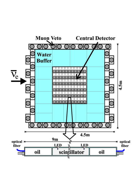
FIG. 1.: The Palo Verde detector. One of the 66 target cells with PMTs, calibration LEDs, and optical fiber flashers is shown lengthwise at the bottom.

The central volume is surrounded on the sides by a 1 m buffer of high purity deionized water (about 105 tons) contained in steel tanks which, together with the oil buffers at the ends of the cells, serve to attenuate gamma radiation from the laboratory walls as well as neutrons produced by cosmic muons passing outside of the detector. The low Z of water minimizes the neutron production by nuclear capture of stopped muons inside the detector and has a high efficiency for neutron thermalization.

The outermost layer of the detector is an active muon veto counter, providing 4$\pi$ coverage. It consists of 32 twelve meter-long PVC tanks (from the MACRO experiment[12]) surrounding the detector longitudinally, and two endcaps. The endcaps are mounted on a rail system to allow access to the central detector. The horizontal tanks are read out by two 5-inch PMTs at each end; the vertical tanks are equipped with one 8-inch PMT at each end while the endcaps use 3-inch PMTs. The liquid scintillator used in the veto is a mixture of 2% pseudocumene and 98% mineral oil, with a light attenuation length at 440 nm in excess of 12 m.

A schematic of the central detector’s front-end electronics is shown in Fig. 2. Each channel can be digitized by either of two identical banks of electronics. The dual bank system allows both parts of the sequential inverse beta decay event to be recorded with no deadtime by switching between banks. Due to the large dynamic range of energy in the data of interest (40 keV to 10 MeV, or 1 to 250 photoelectrons typically), each PMT has both a dynode and anode output connected to ADCs, as well as three discriminator thresholds for the trigger and TDCs. The higher TDC threshold serves to avoid crosstalk from large signals in adjacent channels while the lower threshold allows timing information to still be available at the single photoelectron level. The relative time of arrival from each end of a cell is used to reconstruct longitudinal position. The measured PMT pulse charge at each end, corrected for light attenuation based on the distance traveled in the cell, allows energy reconstruction.

FIG. 2.: Schematic of the front-end electronics. The charge and timing of PMT pulses are read out by two banks of ADCs and TDCs. The timing information is discriminated with two thresholds to avoid crosstalk and retain dynamic range. Trigger discriminator signals from the two PMTs in each cell are or’ed and input to the trigger circuit.

Each cell is connected to the trigger via the or of the discriminated signals from the two PMTs. Signals are tagged according to two thresholds: a high threshold corresponding to $\sim$600 keV for energy deposits in the middle of the cell and a low threshold corresponding to $\sim$40 keV, or one photoelectron at the PMT. The low trigger threshold also serves as the lower TDC threshold. The trigger, which has a decision time for each event of around 40 ns, uses a Field Programmable Gate Array to search for patterns of energy deposits in the central detector, and can be reprogrammed easily to change trigger conditions as needed for calibrations[13].

A veto signal disables the central detector trigger for 10 $\mu$s following the passage of a muon to avoid most related activity. Typical veto rates are $\sim$2 kHz. With each event, the time and hit pattern of the previous muon in the veto counter is recorded along with information as to whether or not the muon passed through the target cells. The veto inefficiency was measured to be (4$\pm$1)% for stopping muons (one hit missed) and (0.07$\pm$0.02)% for through-going muons (two hits missed). We note that the small size of this second quantity with respect to the first is due to correlations between incoming and outgoing muons as confirmed by a simple Monte Carlo model.

B The $\bar{\nu}_{\rm e}$ signal

The $\bar{\nu}_{\rm e}$ signal is detected via the reaction $\bar{\nu}_{\rm e}$p$\rightarrow$ne⁺ as illustrated in Fig. 17 further below along with the dominant backgrounds. Signal events consist of a pair of time-correlated subevents: (1) the positron kinetic energy ionization and two annihilation $\gamma$’s forming the prompt part and (2) the subsequent capture of the thermalized neutron on Gd forming the delayed part. By loading the scintillator with 0.1% Gd, which has a high thermal neutron capture cross section, the neutron capture time is reduced to $\sim$27 $\mu$s from $\sim$170 $\mu$s for the unloaded scintillator. Furthermore, Gd de-excites by releasing an 8 MeV $\gamma$ cascade, whose summed energy gives a robust event tag well above natural radioactivity. In contrast, neutron capture on protons releases only a single 2.2 MeV $\gamma$.

Background is rejected at trigger level using the detector segmentation by looking for coincidences of energy deposits matching the pattern of inverse beta decay. Each of the subevents of a $\bar{\nu}_{\rm e}$ signal is triggered by scanning the detector for a pattern of three simultaneous hits in any 3$\times$5 subset of the cell array. This threefold coincidence, called a triple, must consist of at least one high trigger hit, due to either the positron ionization or neutron capture cascade core, and at least two additional low trigger hits, resulting from either positron annihilation $\gamma$’s or neutron capture shower tails. The use of identical trigger requirements for the two triples is found to give rise to close to an optimal signal to noise ratio. Five $\mu$s after finding an initial triple, the trigger begins searching for a delayed triple. The blank time suppresses possible false signals from PMT afterpulsing. If two triples are found within 450 $\mu$s of each other, the candidate $\bar{\nu}_{\rm e}$ event is digitized for offline analysis.

C Expected $\bar{\nu}_{\rm e}$ interaction rate

In order to calculate the expected $\bar{\nu}_{\rm e}$ interaction rate in the detector, the status of the three reactors is tracked daily, and the fission rates in the cores are calculated based on a simulation code provided by the manufacturer of the reactors. This code uses as input the power level of the reactors, various parameters measured in the primary cooling loop, and the original composition of the core fuel elements.

The output of the core simulation has been checked by measuring isotopic abundances in expended fuel elements in the core; errors in fuel exposure and isotopic abundances are estimated to cause $<0.3$% uncertainty in the $\bar{\nu}_{\rm e}$ flux estimate. Of the four isotopes — ²³⁹Pu, ²⁴¹Pu, ²³⁵U, and ²³⁸U — whose fissions produce virtually all of the thermal power as well as neutrinos, measurements of the neutrino yield per fission and energy spectra exist for the first three[14, 15]. The ²³⁸U yield, which contributes 11% to the final $\bar{\nu}_{\rm e}$ rate, is calculated from theory[16]. When the same theoretical method was used to calculate the spectrum from the other three isotopes, the theory agreed with experimental results within 10%. The contribution of ²³⁸U fission to the overall uncertainty in $\bar{\nu}_{\rm e}$ rate is therefore expected to be $\sim$1%.

FIG. 3.: $\bar{\nu}_{\rm e}$ flux, inverse beta decay cross section, and $\bar{\nu}_{\rm e}$ interaction spectrum at the detector.

This calculated $\bar{\nu}_{\rm e}$ flux is then used to compute the expected rate of $\bar{\nu}_{\rm e}$ candidates $N_{\bar{\nu}_{\rm e}}$ at the detector as a function of the oscillation parameters $\Delta m^{2}$ and $\sin^{2}2\theta$:

$$N_{\bar{\nu}_{\rm e}}=n_{\rm p}\int dE_{\bar{\nu}_{\rm e}}\sigma(E_{\bar{\nu}_{\rm e}})\eta(E_{\bar{\nu}_{\rm e}})\times$$ (3)

$$\sum_{i=1}^{3}\frac{{\mathcal{I}}_{\bar{\nu}_{\rm e},i}(E_{\bar{\nu}_{\rm e}})\left(1-P_{{\rm osc},i}(\Delta{\rm m}^{2},\sin^{2}2\theta,L_{i},E_{\bar{\nu}_{\rm e}})\right)}{4\pi L_{i}^{2}}$$

where $\sigma(E_{\bar{\nu}_{\rm e}})$ is the inverse beta decay cross section[17], $\eta(E_{\bar{\nu}_{\rm e}})$ is the (energy dependent) detector efficiency, $n_{\rm p}$ is the number of target free protons, and ${\mathcal{I}}_{\bar{\nu}_{\rm e},i}$ is the source strength of reactor $i$ at distance $L_{i}$ with oscillation probability $P_{{\rm osc},i}$. In Fig. 3 we show the energy spectrum of the $\bar{\nu}_{\rm e}$’s emitted by a reactor, the $\bar{\nu}_{\rm e}$ (energy) differential cross section in the detector and the actual interaction rate in the detector target before detector efficiency corrections, referred to here as $R_{\bar{\nu}_{\rm e}}$ (obtained by setting $\eta(E_{\bar{\nu}_{\rm e}})$=1). The energy spectrum actually measured in the detector is the energy of the positron created by the inverse beta decay. This spectrum is approximately $E_{\bar{\nu}_{\rm e}}-1.8$ MeV, slightly modified by the kinetic energy carried away by the neutron ($\sim$50 keV).

Previous short baseline experiments which measured the rate of $\bar{\nu}_{\rm e}$ emission by reactors have found good agreement between calculated and observed neutrino flux by using largely the same method of calculation. A high statistics measurement at Bugey[6], in particular, found excellent agreement both in spectral shape ($\chi^{2}/{\rm n.d.f.}$=9.23/11) and in absolute neutrino yield (agreement better than 3%, dominated by systematic errors). These previous generation experiments prove that the reactor antineutrino spectrum, i.e. the $\bar{\nu}_{\rm e}$ flux at the distance $L$=0, is well understood.

The expected $\bar{\nu}_{\rm e}$ interaction rate in the whole target, both scintillator and the acrylic cells, is plotted in Fig. 4 for the case of no oscillations from July 1998 to October 1999. Around 220 interactions per day are expected with all three units at full power. The periods of sharply reduced rate occurred when one of the three reactors was off for refueling, the more distant reactors each contributing approximately 30% of the rate and the closer reactor the remaining 40%. The short spikes of decreased rate are due to short reactor outages, usually less than a day. The gradual decline in rate between refuelings is caused by fuel burnup, which changes the fuel composition in the core and the relative fission rates of the isotopes, thereby affecting slightly the spectral shape of the emitted $\bar{\nu}_{\rm e}$ flux.

FIG. 4.: The calculated $\bar{\nu}_{\rm e}$ interaction rate in the detector target. The two long periods of reduced flux from reactor refuelings were used for background subtraction. The decreasing rate during the full power operation is a result of the changing core composition as the reactor fuel is burned.

III Calibration

In order to maintain constant data quality during running, a program of continuous calibration and monitoring of all central detector cells is followed. Blue LEDs installed inside each cell are used for relative timing and position calibration. Optical fibers at the end of each cell, also illuminated by blue LEDs, provide information about PMT linearity and short term gain changes. LED and fiberoptic scans are performed once a week. Radioactive sources are used to map the light attenuation in each cell, for absolute energy calibration, and to determine detection efficiencies for positrons and neutrons. A complete source scan is undertaken every 2–3 months.

A LED and optical fiber calibrations

As seen in Fig. 1, every cell of the central detector has two LEDs, one at each end at a distance of 90 cm from the PMTs. These blue LEDs, which provide fast light pulses with a rise time comparable to scintillation light, are used for timing calibrations needed for position reconstruction along the cell’s axis.

The difference in pulse arrival time between the two PMTs of a cell $\Delta t$ is described as a function of the position $z$ with an effective speed of light $c_{\rm eff}$, an offset $z_{0}$ and a small nonlinear correction $f(1/Q)$:

$$\Delta t=(z-z_{0})/c_{\rm eff}+f(1/Q_{n},1/Q_{f}).$$ (4)

The correction $f(1/Q_{n},1/Q_{f})$, a function of both near and far PMT pulse charge $Q$, describes the dependence of the pulse height due to time-walk in the leading edge discriminators used in the front-end electronics. To extract these calibration parameters and compensate for the time-walk effect, a third order polynomial is fit to $\Delta t$ versus $1/Q$ (see Fig. 5). The intercepts at $1/Q=0$ for the two LED positions provide $c_{\rm eff}$ and $z_{0}$, while the slopes are used to parameterize the time-walk correction.

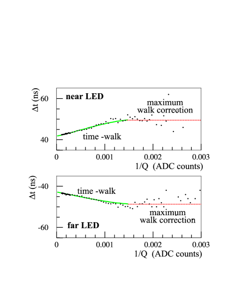
FIG. 5.: Time difference $\Delta t$ as function of $1/Q$ for near- and far-end LEDs of a cell, illustrating the time-walk effect. For values of $Q$ close to the discriminator threshold the time-walk correction is kept at a constant (maximum) level.

In order to check the suitability of longer wavelength 470 nm LED light to measure timing properties of $\sim$425 nm scintillation light, data taken with a ²²⁸Th source at several longitudinal positions were reconstructed with the LED timing calibration parameters. Comparing the reconstructed positions with the actual source positions, the effective speed of light measured with the LED system was found to be on average 3.6% lower than that with the sources. A simulation of the light transport in a cell with various indices of refraction and attenuation lengths of the scintillator suggested that the small discrepancy in $\Delta t$ between LED and scintillation light was due to the difference in attenuation length. The correction factor was found to be constant over several months. Weekly LED scans are therefore used to correct for short term variations in $\Delta t$ and a constant correction factor is applied to the effective speed of light.

The fiberoptic system includes 15 blue LEDs, each illuminating a bundle of 12 fibers. The light output of each LED is measured in two independent reference cells with PMTs checked to be linear over the whole dynamic range of the LEDs. By taking a run which scans through all light intensities and mapping each PMT’s response relative to the reference cells, the nonlinear energy response of the PMTs is calibrated. Low intensities are used to determine the single photoelectron gain of each PMT, which is used to correct for changes from the nominal gain setting of $4\times 10^{7}$.

B Scintillator transparency and energy scale calibration

In addition to weekly LED and fiberoptic calibrations, the energy response of the scintillator is measured every three months using a set of sealed radioactive sources. Eighteen 2.4 mm diameter tubes run along the length of the detector allowing insertion of the sources adjacent to any cell at any longitudinal position. The response of each PMT as a function of longitudinal position is measured by recording the Compton spectrum from the 2.614 MeV $\gamma$ of a ²²⁸Th source at seven different locations along each cell.

Monte Carlo simulation found that the half maximum of a Gaussian function fitted to the Compton spectrum is relatively independent of resolution; this point is therefore used as the benchmark of the cell response. The response versus distance from the PMT, shown in Fig. 6 for one cell, is then fit to the phenomenological function ${\rm exp}(p_{0}+p_{1}z)+{\rm exp}(p_{2}+p_{3}z)/z$, where $z$ is source longitudinal distance from the PMT. The effective attenuation length of the scintillator (including multiple total reflection on the acrylic walls) is generally between 3–4 m and over a year was found to change on average $\sim$1 mm/day, demonstrating that the Gd scintillator was remarkably stable.

FIG. 6.: Effect of aging on Gd loaded scintillator. Top: ²²⁸Th Compton edge position at seven different longitudinal locations along a typical cell. The two curves are from calibrations taken a year apart. The curves are normalized at the location nearest to the PMT. Bottom: Effective attenuation lengths for all 66 cells from the two calibrations.

The overall energy scale was determined from the position of the 1.275 MeV peak of a ²²Na source, and then verified by taking data with several $\gamma$ sources in different energy ranges: ¹³⁷Cs (0.662 MeV), ⁶⁵Zn (1.351 MeV), ²²⁸Th (2.614 MeV), and the capture of neutrons (8 MeV) from an Am-Be source. The gamma cascade from neutron capture was modeled according to measurements of the emitted spectrum[18]. In contrast to homogeneous detectors which measure total absorption energy peaks, 25% of the detector target mass consists of the inert acrylic of the cell walls, which absorbs some energy. The Monte Carlo simulation was therefore used to find the correct final distributions of energy detected from single and multiple scattering of the $\gamma$’s. The total energy reconstructed for data and Monte Carlo for each source is plotted in Fig. 7. The data were matched with Monte Carlo simulation for the ²²Na spectrum in Fig. 12 to find the overall energy scale and to the spectra in Fig. 7 to assure that the scintillator response is linear over the energies of interest. The light yield after PMT quantum efficiency was found to be $\sim$50 photoelectrons per MeV in the center of the cells. The agreement for three of the four sources in Fig. 7 is good, the exception being ²²⁸Th, in which the data has a consistently higher Compton scattering peak than Monte Carlo predicts. This discrepancy is consistent across all the data taken and therefore does not affect the scintillator transparency calibration.

FIG. 7.: The total energy reconstructed for various sources compared for data and Monte Carlo.

C Monte Carlo simulation

The $\bar{\nu}_{\rm e}$ efficiency of the detector is a relatively strong function of event location in the detector and, to a lesser extent, of time due to scintillator aging. A further complication comes from the trigger efficiency being a function of threshold (voltage) while only energy (charge) is measured. For this reason a Monte Carlo model which included a detailed simulation of the detector response, including the PMT pulse shape, is used for an estimate of the overall efficiency for $\bar{\nu}_{\rm e}$ detection. A variety of measurements was performed to crosscheck that the Monte Carlo accurately models the detector response.

The physics simulation program is based on geant 3.21[19]. This code contains the whole detector geometry and simulated the energy, time, and position of energy deposits in the detector. Hadronic interactions are simulated by gfluka[20] and the low energy neutron transport by gcalor[21]. Scintillator light quenching, parameterized as a function of ionization density, is included in the simulation[22].

The event reconstruction program reads the output of this physics simulation and then applies the second step of the Monte Carlo, the simulation of the detector response as PMT pulses which are then converted into time and amplitude digitizations and trigger hits. A logical scheme of this detailed detector simulation is shown in Fig. 8.

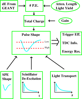
FIG. 8.: Schematic of the Monte Carlo detector simulation program. In order to convert energy deposited into accurate threshold simulation, calibration information from the detector was used to reconstruct PMT pulses.

The calibrations discussed above empirically provide the scintillator light yield (photoelectron/MeV) and attenuation function for each cell, which in turn provide the number of photoelectrons $\overline{N}_{p.e.}$ expected for a simulated energy deposit. The total charge of the pulse then follows from sampling a Poisson distribution with mean $\overline{N}_{p.e.}$ and folding the number of simulated photoelectrons $N_{p.e.}$ with the PMT’s nominal gain, first stage gain variance (10$N_{p.e.}$), and cell-to-cell energy scale calibration uncertainty (10%).

To simulate the pulse shape, an arrival time is assigned to each photoelectron, and individual photoelectron pulses (whose shape is derived from real data) are summed into a final pulse. The calculated arrival time of each photon is a combination of two processes, scintillator de-excitation and propagation along the cell. The latter distribution is parameterized by the distance traveled to the PMT, larger distances giving larger variances, using a light transport simulation of $2\times 10^{7}$ photons. The resulting pulse is then analyzed to extract TDC and trigger hits.

The Monte Carlo threshold simulation, position reconstruction, and positron and neutron efficiency predictions were checked using calibration data. The trigger threshold simulation for each cell was compared to data taken with a ²²Na $\beta^{+}$ source near the center of each cell. The trigger conditions were loosened for these data, a single low hit producing a trigger and the event tagged if a high threshold was crossed. By plotting the reconstructed energy for each event versus the efficiency for a high trigger tag, an effective high trigger threshold in MeV for that location in the cell was determined. The low threshold was measured similarly. The Monte Carlo pulse shape parameters were tuned to these data. A typical cell’s trigger threshold efficiency as a function of energy is shown in Fig. 9 for both data and the Monte Carlo. The trigger threshold, defined as the energy at 50% efficiency, is also plotted for all 66 cells. On average, the thresholds agree to within 1%.

FIG. 9.: A comparison of the trigger thresholds from data and Monte Carlo. The data were taken with a ²²Na source at the center of each cell. The top portion shows the efficiency of the trigger threshold for a typical cell as a function of energy deposited; the bottom shows the energy of the 50% efficiency threshold for all 66 cells.

TDC thresholds were checked by the same algorithm, plotting the threshold hit efficiency versus reconstructed energy. A more direct check of the TDC simulation, however, compares the position reconstruction for data and Monte Carlo simulation. Fig. 10 shows the longitudinal position of the third largest energy deposit in each event for a ²²Na calibration run, representing the position reconstruction of the energy deposited by one of the two positron annihilation $\gamma$’s. Since these energy deposits tend to be small ($\sim$100 keV), some fraction of them have one or both PMT’s responses below the TDC low threshold. These events constitute the tails of the distribution in Fig. 10 since only the relative signal amplitude was used for position reconstruction. The narrower central peak is populated by events with TDC information available. The simulation and data agree well, in both resolution and relative frequency of the two cases.

FIG. 10.: A comparison of the reconstructed $Z$ position of an annihilation gamma energy deposit from a ²²Na run, between data and Monte Carlo. The long tails are due to lower energy deposits which do not have TDC for position reconstruction, in which case relative signal amplitudes are used, resulting in worse resolution. Statistical errors in the plot are negligible.

D $\bar{\nu}_{\rm e}$ detection efficiency

The absolute efficiency of the detector for positron annihilations and neutron captures was verified using ²²Na and Am-Be sources respectively. The ²²Na source emits a 1.275 MeV primary $\gamma$ which is accompanied 90% of the time by a low energy positron which annihilates in the source capsule. The primary $\gamma$ can mimic the positron ionization of a low energy $\bar{\nu}_{\rm e}$ event. This deposit, in conjunction with the positron’s annihilation $\gamma$’s, closely approximates the positron portion of a $\bar{\nu}_{\rm e}$ event near the trigger threshold.

In two rounds of data taking, 10 months apart, the ²²Na source was inserted into the central detector at 35 locations chosen to provide a sampling of various distances from the PMTs and edges of the fiducial volume. The source activity is known to 1.5%, allowing determination of an absolute efficiency. After applying the offline selections used for $\bar{\nu}_{\rm e}$ prompt triples and correcting for detector DAQ deadtime, the measured absolute efficiency was compared with the Monte Carlo prediction; the results are summarized in the top portion of Fig. 11. Good agreement is seen in the average efficiency over all runs, and run by run agreement was 11%.

FIG. 11.: Comparison of data and Monte Carlo detection efficiency for Am-Be and ²²Na source runs at various locations. Locations at the edges of the detector tend to have lower efficiencies.

The energy spectra predicted by the simulation and measured in the data for the ²²Na runs were compared. The total energy seen in all cells and the energy detected in the three most energetic hits are plotted in Fig. 12. The trigger thresholds can be seen in the spectra: the high trigger threshold is the rising edge at around 0.5 MeV in the spectrum of the most energetic hit (E₁), and the low trigger threshold is the rising edge at around 50 keV of the third most energetic hit (E₃).

FIG. 12.: The Monte Carlo simulation and the data compared for the spectra of total energy and first, second, and third most energetic hit ($E_{\rm total}$, $E_{1}$, $E_{2}$, and $E_{3}$) digitized in the ²²Na calibration runs.

A similar procedure was used to check the neutron capture detection efficiency. The Am-Be neutron source is attached to one end of a thin (7.5mm) NaI(Tl)-detector, which tagged the 4.4 MeV $\gamma$ emitted in coincidence with a neutron. The NaI(Tl) tag forces the digitization of the 4.4 MeV $\gamma$ as the prompt part of an event and opens a 450 $\mu$s window for neutron capture; this is the same coincidence window used in the $\bar{\nu}_{\rm e}$ runs.

All neutron cuts used for the $\bar{\nu}_{\rm e}$ data selection were applied, and the resulting detection efficiency was corrected for detector deadtime and a small random coincidence background. On average, the Monte Carlo efficiency predictions agrees well over the 25 locations tested with a run by run agreement of better than 4%, as shown in the bottom of Fig. 11.

As with the ²²Na runs, the energy spectra predicted by the simulation and measured in the data were compared. The total energy seen in all cells and the energy detected in the three most energetic hits is plotted in Fig. 13. Note the small peak in $E_{\rm total}$ at $\sim$2 MeV arising from neutrons being captured on hydrogen. The differences in data versus Monte Carlo spectra for ²²Na and Am-Be were taken into account in estimating systematic errors.

FIG. 13.: The Monte Carlo simulation and the data compared for the spectra of total energy and first, second, and third most energetic hit ($E_{\rm total}$, $E_{1}$, $E_{2}$, and $E_{3}$) digitized in the Am-Be calibration runs.

The Am-Be source emits neutrons with kinetic energies up to 10 MeV, creating proton recoils in the detector scintillator in coincidence with the NaI(Tl) induced trigger. By digitizing any energy deposits seen during the neutron release, the high ionization density of these recoiling protons was used in setting the parameters which control scintillator light quenching in the simulation.

The above crosschecks verify our ability to accurately generate the events, model the detector response, reconstruct the events, and correctly calculate the livetime of the data acquisition (DAQ) system. Taken together these procedures complete the task of estimating our $\bar{\nu}_{\rm e}$ efficiency.

The Monte Carlo simulation for $\bar{\nu}_{\rm e}$ events models the expected interactions throughout the entire target, including the acrylic walls of the cells, since there is significant efficiency for inverse beta decay originating in the acrylic. The Monte Carlo simulation yields an average efficiency over the entire detector as a function of $\bar{\nu}_{\rm e}$ energy. The efficiency from the simulation is folded with the incident $\bar{\nu}_{\rm e}$ spectrum (which may be distorted by oscillations depending on the hypothesis tested), to get the effective efficiency.

E An independent reconstruction and Monte Carlo

A parallel and independent event reconstruction and the simulation of the detector response has been developed. This second version follows the same general outline of detector calibration, event reconstruction, and simulation described above, but differs in the algorithms and parameterizations used. Major differences include:

• The functional form for the scintillator light attenuation is the sum of two exponentials ${\rm exp}(p_{0}+p_{1}z)+{\rm exp}(p_{2}+p_{3}z)$, without $z^{-1}$ in the second term.

• The cell response benchmark is the 70% maximum rather than half maximum of the fitted Compton scattering spectrum.

• A different parameterization is used for the linearity correction of the dynode signals.

• The low threshold parameters are tuned to the TDC hit efficiencies rather than trigger efficiencies as discussed above.

• An alternate algorithm for simulating the PMT pulse shape was developed and tuned to observed PMT pulse characteristics.

These differences manifest themselves as slightly different $\bar{\nu}_{\rm e}$ efficiency predictions and $\bar{\nu}_{\rm e}$ candidate rates in the data. Tests with radioactive sources have been performed to evaluate the quality of the second data reconstruction. The ²²Na and Am-Be efficiency runs shown in Fig. 11 were reconstructed by the second analysis to test its efficiency prediction throughout the detector. The ratio of predicted to observed efficiencies over all the e⁺ and neutron runs for the first reconstruction (1) and the second reconstruction (2) are plotted in Fig. 14. While the results presented in the analyses below come from the first reconstruction code described above, the development of a second simulation and event reconstruction offers a useful crosscheck of the systematic uncertainties of the results. The differences between the two analyses were used to corroborate the estimate of systematic errors.

FIG. 14.: The ratio of predicted to observed efficiency of ²²Na and Am-Be for the two reconstruction codes (1) and (2).

IV $\bar{\nu}_{\rm e}$ selections and backgrounds

A $\bar{\nu}_{\rm e}$ selection

The trigger rate for time-correlated events (two triples occurring within 450 $\mu$s) is $\sim$1 Hz. Most of those events are random coincidences of two uncorrelated triple hits, which occur individually at a rate of $\sim$50 Hz, mostly from natural radioactivity. In order to select neutrino events, the following offline cuts are applied:

• The energy reconstructed in both prompt and delayed triples has at least one hit with $E>$1 MeV and at least two additional hits with $E>$30 keV. No single hit was allowed to be greater than 8 MeV.

• The prompt triple is required to resemble a positron, i.e. annihilation $\gamma$’s each less than 600 keV, and together less than 1.2 MeV. (This cut is the only one which treats the two triples asymmetrically).

• At least one of the two triples in the event has more than 3.5 MeV of reconstructed energy for rejection of $\gamma$ backgrounds.

• The prompt and delayed portions of the event are correlated in space and time (within 3 columns, 2 rows, one meter longitudinally, and 200 $\mu$s).

• The event started at least 150 $\mu$s ($\sim$5 neutron capture times) after the previous veto tagged muon activity.

The trigger and selection efficiencies are summarized in the first two columns of Table I.

	Cumulative		Data
Cut	efficiency		Rate (d-1)
	1998	1999	1998	1999
Trigger	0.271	0.328	69k	106k
Selection Cuts	0.149	0.177	1k	1.2k
Liveμveto	0.102	0.121	$<$50, see
LiveDAQ:	0.075	0.112	Table V

TABLE I.: Summary of efficiency and data rates after trigger, selections, and live time. The entry “Live_μveto” refers to the dead-time induced by the 150 $\mu$s blanking window that accompanies each muon detected in the veto counter.

In addition to corrections for selection cut efficiency and trigger efficiency, detector livetime is a substantial correction to the number of neutrinos seen and deserves some comment. Deadtime comes from two sources, the DAQ and the muon veto. DAQ livetime is the ratio of the number of triples the DAQ was available for digitizing to the total number of triples the trigger saw. These numbers are available from trigger scalers. The trigger livetime was measured to be $>$99.9%. The DAQ live time varies with the triple rate, and for the four data periods was determined to be 73.2%, 74.4%, 92.3%, and 91.8% for 1998 full power, 1998 refueling, 1999 full power, and 1999 refueling, respectively. The higher livetime in 1999 is due to improvements made in the trigger conditions.

The muon deadtime can be further divided into two contributions: 150 $\mu$s of deadtime caused by each muon, which at $R_{\mu}=$ 1990 Hz left the detector live 74.2% of the time; and muons which interrupted a neutrino event between the positron and the neutron capture, which estimated from the fit parameters of the Monte Carlo capture time left 92.5% of events uninterrupted. The total uncertainty in the calculation of detector deadtime is less than 1%

B Backgrounds

Backgrounds can be separated into two types: correlated and uncorrelated. Uncorrelated background events are due to unrelated triple hits which randomly coincided in the time window allowed. Although most of the events collected were random coincidences, almost all of this type of background is removed by requiring at least one subevent to have more than 3.5 MeV of reconstructed energy. These events do not have a time correlation between prompt and delayed subevents (inter-event time) characteristic of neutron capture. They have instead a longer time correlation determined by the probability that the veto detected no muon between the prompt and delayed random triples. At a 2 kHz muon rate, this background is seen as a 500 $\mu$s tail under the normal neutron capture distribution. By looking at the inter-event times of the candidate $\bar{\nu}_{\rm e}$ events at longer time scales, this background can be measured.

The inter-event time distribution after all neutrino selections (except the time correlation cut) is shown in Fig. 15. The Monte Carlo for a pure neutron capture sample is empirically fitted to the sum of two exponentials. There are two time constants due to the inhomogeneity of the target: neutrons which remain in the scintillator have a 27 $\mu$s capture time, whereas those which enter the acrylic have a longer capture time due to the absence of Gd. The data inter-event time distribution is fitted to a function of three exponentials with fixed time constants consisting of the Monte Carlo fit $\tau$’s multiplied by a third time constant of 500 $\mu$s. Integrating the resulting 500 $\mu$s exponential of the uncorrelated background in the signal region gives an estimate of 4.1$\pm$0.2 events per day, or 9% of the $\bar{\nu}_{\rm e}$ candidates being uncorrelated background events.

FIG. 15.: The time elapsed between the prompt and delayed portion of neutrino candidate events for Monte Carlo simulation and data. The Monte Carlo is fit to two exponentials. The data are fit to three exponentials, constrained to have the time structure of the simulation and an additional contribution due to uncorrelated background (dashed line).

To measure the uncorrelated background in smaller parts of the data set, the statistical accuracy of the three exponential fit method becomes unacceptably poor. A simpler method is therefore used in conjunction with the above fit. For inter-event times longer than 200 $\mu$s, the $\bar{\nu}_{\rm e}$ candidates are dominated by uncorrelated backgrounds. The integrated number of candidates from 200–400 $\mu$s is scaled to estimate the number underneath the signal region ($<$200 $\mu$s). Using the scaling from the fit of the entire data set shown in Fig. 15, the uncorrelated background was measured in approximately month-long intervals as shown in Fig. 16. For both the 1998 and 1999 data sets, the rates are found to be stable within statistical errors.

FIG. 16.: The uncorrelated background rate as measured in approximately month-long segments of the data. Overlain is a fit to a constant within each year’s data; the fit quality is consistent with a stable background.

Correlated backgrounds have the neutron capture inter-event time structure of the $\bar{\nu}_{\rm e}$ candidates. These events come mainly from cosmic muon induced fast neutrons from spallation or muon capture, as shown schematically in Fig. 17. These fast neutrons can either (1) induce more neutrons via spallation, two of which can be captured in the detector with one capture mimicking a positron signature; or (2) they can cause proton recoil patterns in the central detector which appear as a positron signature and then get captured. Spallation neutrons originate from muons passing through the walls of the lab without hitting the veto detector or from muons passing through the detector shielding undetected by the veto. Muon capture neutrons mainly originate from muons stopping in the water buffer without registering in the veto.

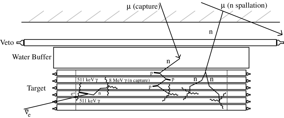
FIG. 17.: A schematic drawing of the detector showing a signal event and two examples of interactions which contribute to the correlated background. Neutrons which cause correlated backgrounds come mainly from muons undetected by the veto and captured in the water buffer (left), and spallation from muons in the lab walls (right). These neutrons in turn can either induce more neutrons via spallation (as shown at right) or cause three coincident proton recoils as they thermalize (as shown at left).

FIG. 18.: The time between the previous muon traversing the veto counter and a neutrino candidate event trigger. The fit is to a sum of three exponentials. The dashed portion denotes events uncorrelated to the previous muon, the rest are correlated background events induced by cosmic muons. The neutron capture time constants, shorter than the simulation prediction for $\bar{\nu}_{\rm e}$ events, imply multiple neutron production.

To illustrate some properties of correlated background, Fig. 18 shows the time elapsed since the previous veto hit for $\bar{\nu}_{\rm e}$ candidates, with all selection cuts applied except that of the previous muon timing. This distribution is fit to a three exponential function analogous to that used for the inter-event time fits. The two time constants for neutron capture are not identical to those for $\bar{\nu}_{\rm e}$ events, but tend to be smaller since after passage of a muon there are often more than one neutron in the detector to be captured. The third exponential time constant is again constrained to 500 $\mu$s as expected in a random sampling of events unrelated to the previous muon. Since at very short times there are other contributions such as muon decay, times less than 15 $\mu$s are excluded from the fit. Muon-induced-neutron backgrounds dominate the candidates in the first 150 $\mu$s after the previous tagged muons, motivating the selection cut on $\mu$ timing.

In order to show that the correlated background was constant in time, the previous muon time cut was disabled and a plot was made of the $\bar{\nu}_{\rm e}$ candidate rate versus time, as shown in Fig. 19. When fit to a constant for each year, a $\chi^{2}$/n.d.f. of 382.7/371 is obtained, which has a 33% likelihood, indicating that the detector efficiency for correlated backgrounds was stable during each year’s data taking.

FIG. 19.: The number of candidates per day in the 373 runs used in this analysis, fit to a constant for each year. All neutrino selections except the previous muon time cut are used, leaving a data set dominated by muon-induced-neutron background. The different rates in 1998 and 1999 are due to trigger and livetime improvements.

Aside from the detector efficiency for background, however, a loss of veto efficiency could also cause a fluctuation in background. (The rates fit in Fig. 19 are with the muon timing selection disabled, and hence do not vary with veto inefficiency.) To track veto efficiency, the veto hit patterns recorded with each event are used. If a muon hit was recorded only on the bottom of the veto, where only exiting muons are seen, then the muon must have entered the veto without recording a hit. By measuring the percentage of these events a one hit missed veto inefficiency of ($4\pm 1$)% is found as mentioned above. The through-going (two hits missed) veto inefficiency is measured to be $0.07\pm 0.02\%$ by looking at the rate of $\mu$ tracks triggered on in the central detector. These inefficiencies were tracked in time to assure their stability.

C Neutron–$\bar{\nu}_{\rm e}$ direction correlation

The neutrons produced in the inverse beta decays will have momenta slightly biased away from the source, whereas no correlation is expected for background. This effect is the consequence of momentum conservation which requires that the neutron should always be emitted in the forward hemisphere with respect to the incoming $\bar{\nu}_{\rm e}$. Such a correlation has been observed already in the Gösgen experiment[23] and again at Chooz[24]. The theoretical treatment of the effect can be found in [17].

The signal to background ratio can be independently verified using this effect. The $\bar{\nu}_{\rm e}$ source is to the left of the detector in Fig. 1. The relative horizontal location (relative column in the target cell array) of neutron capture cascade cores versus positron ionizations for data and the simulation of the $\bar{\nu}_{\rm e}$ signal are plotted in Fig. 20. Defining the asymmetry $A_{\rm data}=\frac{R-L}{R+L}$ in terms of the number of neutrons captured one column away from the source $R$ and one column toward the source $L$, a slight asymmetry $0.050\pm 0.017$ is found in the data, at 2.9 $\sigma$ significance. Using the Monte Carlo simulation which gives $A_{\rm MC}=0.134$ to estimate the portion of the data consisting of $\bar{\nu}_{\rm e}$ signal and assuming the background to be symmetric in this variable, an effective signal to noise ratio

$$\frac{S}{N}=\frac{A_{\rm data}}{A_{\rm MC}-A_{\rm data}}=0.6^{+0.4}_{-0.3}$$ (5)

is found. This value agrees well with the ratio of $0.81\pm 0.03$ found with the swap analysis method described below.

FIG. 20.: The relative horizontal location of the neutron capture and positron ionization in the detector target. The kinematics of the inverse beta decay cause a slight bias in the momentum of the neutron from inverse beta decay, seen here as an asymmetry in the populations of neutrons captured one column away or towards the $\bar{\nu}_{\rm e}$ source. Backgrounds should not exhibit such asymmetry. The Monte Carlo prediction for the pure $\bar{\nu}_{\rm e}$ signal, normalized to unity, is also plotted.

V Analysis

The data set presented here was taken from July 1998 to September 1999 in 373 short runs, each on average about 12 hours long. In 1998, 35.97 days of data were taken with the three reactors at full power and 31.35 days with one of the reactors at a distance of 890 m off for refueling. The detector was then taken offline in Jan/Feb of 1999, when DAQ improvements were made to increase livetime, and the high trigger thresholds were lowered by 30% to increase trigger efficiency. The 1999 data set includes 110.95 days with all three reactors at full power and 23.40 days with the 750 m baseline reactor off for refueling. Thus, the entire data set has four distinctly different periods, with three different baseline combinations and neutrino fluxes.

After all selection cuts there is still substantial background in the remaining data set. The correlated background, coming mainly from muon induced neutrons, is difficult to predict and subtract. The yield and spectrum of neutron spallation is a function of muon flux and energy, which in turn is a function of depth. While some measurements of fast neutron spectra and fluxes have been done in the past, there is no model which can consistently predict the fast neutron production. Below we present three methods used to extract the $\bar{\nu}_{\rm e}$ signal from data.

A Analysis with the on-off method

The conceptually simplest method of subtracting background is to take advantage of periods of reduced power levels of the reactor source. Ideally all three reactors would be down at once allowing for a direct measurement of the background. However, in practice only one of the three Palo Verde reactors was refueled at any given time. These reduced power periods occurred twice annually for about a month. Each year’s data set is treated independently, subtracting 1998 off from 1998 on and 1999 off from 1999 on, since the efficiency of the detector changed between the two years. By subtracting these data taken at reduced flux from the full flux data, a pure neutrino sample is retrieved albeit containing the statistical power of only a small portion of the potential data set: the subtraction is limited by the two months of refueling time and treats the $\bar{\nu}_{\rm e}$ flux from the two reactors still at full power as background.

The primary concern arising from use of this method, aside from the loss of statistics, is guaranteeing that the background rates during the on and off periods were stable. Both correlated and uncorrelated backgrounds were carefully tracked to ensure stability as discussed above.

	1998	1999
$L$ (m)	890	750
ON $N_{\rm cand}$ (day-1)	$38.2\pm 1.0$	$52.9\pm 0.7$
OFF $N_{\rm cand}$ (day-1)	$32.2\pm 1.0$	$43.9\pm 1.4$
ON-OFF $N_{\rm cand}$ (day-1)	$6.0\pm 1.4$	$9.0\pm 1.6$
Total efficiency ON (OFF)	0.0746 (0.0772)	0.112 (0.111)
$R_{\rm obs}$ (day-1)	$95\pm 19$	$77\pm 14$
$R_{\rm calc}$ (day-1)	63	88

TABLE II.: Results for the simple on-off background subtraction analysis, showing candidate rates in the data $N$ and efficiency corrected $\bar{\nu}_{\rm e}$ interaction rates $R$ observed and calculated. The data sets for each year are considered independently here. Uncertainties are statistical only. Systematic errors are estimated to be 10%.

The numerical results of this analysis of the total rate are summarized in Table II. After correcting for efficiency (for the no-oscillations scenario) and livetime, the data sets were subtracted to find observed neutrino interaction rates in the detector. No significant deviation from the expected neutrino interaction rates was found at either baseline distance.

The results from the alternate reconstruction (2) for this analysis are shown in Table III for comparison. This analysis selects about 5% more candidates, but also gives a correspondingly higher efficiency. For this analysis, the uncorrelated background was measured and removed from the data before the subtraction.

	1998	1999
$L$ (m)	890	750
ON $N_{\rm cand}$ (day-1)	$37.3\pm 1.2$	$49.3\pm 0.7$
OFF $N_{\rm cand}$ (day-1)	$31.6\pm 1.2$	$38.6\pm 1.6$
ON-OFF $N_{\rm cand}$ (day-1)	$5.7\pm 1.7$	$10.7\pm 1.8$
Total efficiency ON (OFF)	0.0809 (0.0838)	0.121 (0.121)
$R_{\rm obs}$ (day-1)	$85\pm 20$	$89\pm 15$
$R_{\rm calc}$ (day-1)	63	88

TABLE III.: Results from the alternate reconstruction (2) for the simple on-off background subtraction analysis. Uncorrelated background was accounted for in the the data before subtraction. Uncertainties are statistical only. Systematic errors are estimated to be 10%.

In order to test the results for oscillation hypotheses in the two flavor $\Delta m^{2}-\sin^{2}2\theta$ plane, a $\chi^{2}$ analysis is performed comparing the calculated $R_{{\rm calc},ij}$ and observed $R_{{\rm obs},ij}$ spectra divided into 1 MeV bins $j$ for each year $i$. The spectra used are the prompt energies of the two subtracted data sets. At each point in the oscillation parameter plane, taking into account the changes in detector efficiency due to distortions of the neutrino spectrum, the quantity

$$\chi^{2}=\sum_{i=1}^{2}\sum_{j}^{E_{\rm bins}}\frac{\left(\alpha R_{{\rm calc},ij}-R_{{\rm obs},ij}\right)^{2}}{\sigma_{ij}^{2}}+\frac{(\alpha-1)^{2}}{\sigma_{\rm syst}^{2}}$$ (6)

is computed, where $\alpha$ accounts for possible global normalization effects due to systematic uncertainties (discussed below) across both periods and $\sigma_{ij}$ is the statistical uncertainty in each bin. Systematics which can affect spectral shape, mainly energy scale uncertainty, are negligible relative to the statistical uncertainties in the analysis. The function is minimized with respect to $\alpha$. The point in the physically allowed parameter space with the smallest chi-square $\chi^{2}_{\rm best}$ was found, which represents the oscillation scenario best fit by the data.

The 90% confidence level (CL) acceptance region is defined according to the procedure suggested by Feldman and Cousins[25] by:

$$\Delta\chi^{2}=\chi^{2}(\Delta m^{2},\sin^{2}2\theta)-\chi^{2}_{\rm best}>\\ \Delta\chi^{2}_{\rm crit}(\Delta m^{2},\sin^{2}2\theta)$$ (7)

where $\chi^{2}(\Delta m^{2},\sin^{2}2\theta)$ is the minimized fit quality at the current point in $\Delta m^{2}-\sin^{2}2\theta$ space and $\Delta\chi^{2}_{\rm crit}$ is the CL $\chi^{2}$ cutoff. Due to the sinusoidal dependence of the expected rates on the oscillation parameters and the presence of physically allowed boundaries to those parameters, the cutoff is not simply the $\Delta\chi^{2}$ one would analytically find for a three parameter minimization but has to be calculated for each point in the plane. To find the $\Delta\chi^{2}_{\rm crit}$ for a point, the experiment is simulated $10^{4}$ times under the assumption that the oscillation hypothesis represented by that point is true. For each simulated data set, a $\chi^{2}_{\rm best}$ is extracted and a $\Delta\chi^{2}$ found for the point. These 10⁴ $\Delta\chi^{2}$, the simulations’ fit qualities to the hypothesis, are then ordered. The $\Delta\chi^{2}$ of which 90% of the simulations are a better fit is a 90% CL and therefore that oscillation hypothesis’ $\Delta\chi^{2}_{\rm crit}$.

The region excluded by the analysis is shown in curve (a) of Fig. 21. The results of the $\chi^{2}$ analysis, including the oscillation parameters’ best fit to the data, are summarized in the first column of Table VI further below. For the on-off analysis a best fit preferring the no-oscillation hypothesis was found.

In addition to the analysis of the absolute $\bar{\nu}_{\rm e}$ rates observed, one can analyze the shape of the spectrum of neutrinos seen independently of the absolute normalization, thereby relieving the result of most systematic uncertainties. The $\chi^{2}$ is calculated at each point in the oscillation parameter plane as in Eqn.( 6), with no constraint on normalization ($\sigma_{\rm syst}\rightarrow\infty$). The same procedure as before is followed in defining a 90% CL region in the $\sin^{2}2\theta$–$\Delta m^{2}$ plane. At large $\Delta m^{2}$ where $\bar{\nu}_{\rm e}$ of all energies are oscillating many times within the baseline, the energy spectrum of the incident flux is affected only in magnitude. As a result, the region excluded in the plane does not extend to large $\Delta m^{2}$, as shown in Fig. 21 (b).

FIG. 21.: 90% CL limits of the on-off analysis. (a) on-off subtraction with normalization constraint, and (b) using only the spectral shape.

For the spectrum analysis, when the normalization $\alpha$ is left free, the minimum $\chi^{2}$ is obtained for $\alpha\sim 2$ (see Table VI) and maximum mixing. This is clearly an unphysical result since such large value of $\alpha$ can be excluded to a very high degree of confidence by the independent efficiency calibrations of the detector discussed in previous sections. In addition this result has no effect on the exclusion plot in Fig. 21 because, as shown in Table VI the no-oscillation hypothesis has actually better $\chi^{2}/{\rm n.d.f.}$ than the minimum. Also the exclusion plots based on Eqn. (7) and either $\chi^{2}_{\rm best}$ or $\chi^{2}_{\rm no.osc.}$ are found to be virtually identical. Furthermore, changing the bin size from 1 MeV to 0.5 MeV does not appreciably change the exclusion plot, either.

Since the analyses reported above and in the following sections finds no evidence for neutrino oscillations, the spectra of the two years are added and the summed spectrum is plotted in Fig. 22 along with the Monte Carlo expectation.

FIG. 22.: Total energy of the prompt subevent ($\sim E_{\bar{\nu}_{\rm e}}-1.8$ MeV) in 1 MeV wide energy bins (observed and expected for no oscillation) from the on-off analysis, summed over 1998 and 1999. The spectra are in agreement with each other, with a $\chi^{2}$/n.d.f. = 8.5/8. Uncertainties are statistical only.

B Analysis with the reactor power method

Part of the statistical limitations of the direct subtraction of the preceding analysis is a result of the separation of the data set by year. By correcting the four periods for efficiency and then subtracting the respective reduced flux from full flux periods, the subtraction is forced to treat the $\bar{\nu}_{\rm e}$ flux from two of the reactors as background. A second $\chi^{2}$ analysis was performed which effectively uses the full $\bar{\nu}_{\rm e}$ flux of the refueling periods.

To use the 1998 and 1999 data sets together, the change of both signal and background efficiencies are accounted for. The $\bar{\nu}_{\rm e}$ efficiency difference is found through the detector Monte Carlo simulation. The efficiency change for background from 1998 to 1999, which is not necessarily the same as for $\bar{\nu}_{\rm e}$, is extracted via the high statistics fits of correlated background shown in Fig. 19. The 27% increase in background efficiency observed roughly corresponds to what the Monte Carlo simulation predicts for a background composed mainly of double neutron captures. Uncorrelated background accounts for less than 10% of the candidate set; this background’s efficiency changed by a similar amount within the measurement statistics seen in Fig. 16.

The combined data sets are analyzed for oscillation hypotheses by calculating the $\chi^{2}$ summed over runs $i$ (runs with less than ten candidates are combined with adjacent runs):

$$\chi^{2}=\sum_{i}\frac{\left((\alpha N_{{\rm calc},i}+b)-N_{{\rm cand},i}\right)^{2}}{\sigma_{i}^{2}}+\frac{(\alpha-1)^{2}}{\sigma_{\rm syst}^{2}}.$$ (8)

where $N_{{\rm cand},i}$ is the total $\bar{\nu}_{\rm e}$ candidate rate, $N_{{\rm calc},i}$ is the calculated rate, $\alpha$ is the overall normalization as before, and $b$ is the background rate. The background, $b$, is scaled as appropriate for the year but is otherwise assumed to be constant. The function is minimized at each point with respect to $b$ and $\alpha$. We found no evidence for oscillations and the 90% CL plot, shown in Fig. 23, curve (a), is then constructed around the $\chi^{2}_{\rm best}$ as before by comparing $\Delta\chi^{2}$ with $\Delta\chi^{2}_{\rm crit}$ at each point. The predictions of signal and background from this fit for the no-oscillation hypothesis are shown in Table IV. The no-oscillation likelihood and best fit results of the $\chi^{2}$ analysis with this method are summarized in the third column of Table VI.

Events	1998 ON	1998 OFF	1999 ON	1999 OFF
(day-1)		(890 m)		(750 m)
$N_{{\rm cand}}$	38.2$\pm$1.0	32.2$\pm$1.0	52.9$\pm$0.7	43.9$\pm$1.4
$b$	$19.5\pm 1.7$		$26.3\pm 2.2$
$N_{{\rm detected}}$	18.7$\pm$2.0	12.7$\pm$2.0	26.6$\pm$2.3	17.6$\pm$2.6
$R_{{\rm obs}}$	225$\pm$24	140$\pm$22	216$\pm$19	140$\pm$21
$R_{{\rm calc}}$	218	155	218	130

TABLE IV.: The rate of candidates $N_{{\rm cand}}$, signal $N_{{\rm detected}}$, and background $b$ found by the reactor power analysis, using a $\chi^{2}$ analysis of the data set run by run. The efficiency-corrected total interaction rates $R$ are also listed. Errors are statistical only. The systematic uncertainty is estimated to be 10%.

C Analysis with the swap method

A third analysis is used which has the potential of using the full statistical power of the neutrino data set by subtracting background directly. The method, discussed in more detail elsewhere[26], takes advantage of the asymmetry of the prompt (positron) and delayed (neutron capture) subevents of the neutrino signal. The data selection and trigger treat the two portions of the event identically with the exception of two cuts designed to isolate events with annihilation-like $\gamma$’s in the prompt triple.

The candidates remaining after the selection cuts can be written as:

$$N=B_{\rm unc}+B_{\rm nn}+B_{\rm pn}+S_{\nu}$$ (9)

where $B_{\rm unc}$, $B_{\rm nn}$, and $B_{\rm pn}$ are uncorrelated, two-neutron, and proton-recoil–neutron-capture backgrounds respectively; and $S_{\nu}$ is the neutrino signal. Applying the same neutrino cuts with the positron cuts reversed, or swapped, (such that the positron cuts are now applied to the delayed triple) gives:

$$N^{\prime}=B_{\rm unc}+B_{\rm nn}+\epsilon_{1}B_{\rm pn}+\epsilon_{2}S_{\nu}$$ (10)

Since the uncorrelated background and two neutron capture backgrounds are symmetric under exchange of the prompt and delayed triples, their efficiencies with the reversed cuts remain the same. The parameters $\epsilon_{1}$ and $\epsilon_{2}$ denote the relative efficiency change for proton recoils and neutrino signal under the swap, respectively.

The positron cuts are highly efficient for positron annihilation events but have poor efficiency for neutron captures. The Monte Carlo simulation is used to estimate $\epsilon_{2}=0.159$. Subtracting (9) from (10) leaves the majority of the neutrino candidates and only proton recoil background:

$$N-N^{\prime}=(1-\epsilon_{1})B_{\rm pn}+(1-\epsilon_{2})S_{\nu}.$$ (11)

To estimate $(1-\epsilon_{1})B_{\rm pn}$, it is noted that the proton recoil spectrum extends beyond 10 MeV, well above the positron energies of the neutrino signal and other sources of background. These measured high energy events can be used to normalize the $B_{\rm pn}$ background in the signal using the Monte Carlo ratio:

$$r\equiv\frac{B_{\rm pn}^{\rm MC}({\rm E}_{\rm 1,e^{+}}<8{\rm MeV})}{B_{\rm pn}^{\rm MC}({\rm E}_{\rm 1,e^{+}}>10{\rm MeV})},$$ (12)

where $B_{\rm pn}^{\rm MC}({\rm E}_{\rm 1,e^{+}}<8{\rm MeV})$ is the fraction of simulated $B_{\rm pn}$ events passing the normal $\bar{\nu}_{\rm e}$ selections, and $B_{\rm pn}^{\rm MC}({\rm E}_{\rm 1,e^{+}}>10{\rm MeV})$ are the fraction of simulated events in the high energy background region. Multiplying the ratio $r$ by the measured high energy proton recoil rate gives the $B_{\rm pn}$ background contribution:

$$B_{\rm pn}=rB_{\rm pn}^{\rm data}({\rm E}_{\rm 1,e^{+}}>10{\rm MeV}).$$ (13)

Period	1998 ON	1998 OFF	1999 ON	1999 OFF
		890 m reactor off		750 m reactor off
time (days)	35.97	31.35	110.95	23.40
$\bar{\nu}_{\rm e}$ overall efficiency (%)	7.46	7.72	11.2	11.1
$B_{\rm pn}^{\rm data}({\rm E}_{\rm 1,e^{+}}>10{\rm MeV})$(day-1)	8.79	9.09	13.52	13.29
$(1-\epsilon_{1})B_{\rm pn}$(day-1) $\mu$ spallation	-0.88	-0.91	-1.35	-1.33
$(1-\epsilon_{1})B_{\rm pn}$ (day-1) $\mu$ capture	0.58	0.58	0.86	0.86
$N$ (day-1)	$38.2\pm 1.0$	$32.2\pm 1.0$	$52.9\pm 0.7$	$43.9\pm 1.4$
$N^{\prime}$ (day-1)	$24.6\pm 0.8$	$21.2\pm 0.8$	$32.3\pm 0.5$	$31.7\pm 1.2$
$\mathrm{N}_{\nu}$ (day-1)	$16.5\pm 1.4$	$13.5\pm 1.4$	$25.1\pm 0.9$	$15.0\pm 1.9$
Total background $B_{\rm unc}+B_{\rm nn}+B_{\rm pn}$ (day-1)	$21.7\pm 1.0$	$18.7\pm 1.0$	$27.8\pm 0.6$	$28.8\pm 1.3$
$R_{{\rm obs}}$ (day-1)	$221\pm 19$	$174\pm 17$	$225\pm 8$	$137\pm 17$
$R_{{\rm calc}}$ (day-1)	218	155	218	130

TABLE V.: Results for the swap analysis, including the various background estimates. Uncertainties are statistical only.

The neutrons which cause the proton recoil background are created either by muon capture or spallation in the laboratory walls, or by muons entering the veto counter undetected. The spectrum of the fast neutrons from spallation is not well understood. However, such spectrum can be decoupled somewhat from the resulting proton recoil spectrum. The expected backgrounds were simulated for various possible fast neutron spectra and the resulting $\epsilon_{1}$ and $r$ for neutrons created in the lab walls were calculated. The same calculation was performed for neutrons created in the passive detector shielding by untagged muons; in this case, the expected yield is much smaller, being only a few percent of that from the walls. The simulated spectra of spallation neutrons are chosen to span the wide range of predictions quoted in literature.

A value for $\epsilon_{1}$ of $1.14\pm 0.07$ is found after averaging over spectra, implying that the spallation proton recoil background is essentially symmetric like the other backgrounds. Upon simulating the possible spectra, the quantity $(1-\epsilon_{1})r=0.1\pm 0.05$ is found to vary little.

The yield and spectrum of neutrons from muon capture are reasonably well understood. Since these neutrons tend to be lower in energy, only those created in the vicinity of the detector have any efficiency for creating background. Knowing the veto inefficiency to miss stopping muons ($4\pm 1$)%, the capture rate in water surrounding the detector and its contribution to the background can be estimated using Monte Carlo simulation. Overall this proton recoil background appears to be symmetric as well, $\epsilon_{1}=0.77\pm 0.32$, meaning that the subtraction also strongly rejects this background. The uncertainty of the residual background $(1-\epsilon_{1})B_{\rm pn}$ is conservatively estimated to be about 160%, corresponding to $\sim$4% error on $N_{\bar{\nu}_{\rm e}}$.

The results of this analysis are summarized in Table V. Overall

$$\frac{R_{\rm obs}}{R_{\rm calc}}=1.04\pm 0.03({\rm stat.})\pm 0.08({\rm sys.}).$$ (14)

The background estimates returned by the reactor power analysis in Table IV compare well with the results of the swap analysis. The 90% CL region for this analysis follows the same $\chi^{2}$ formula, Eqn. 8, as for the reactor power analysis but uses the background estimated by the swap method subtraction instead of minimizing the function with respect to background. Again, we find no evidence for neutrino oscillations and the excluded region for this analysis is shown in Fig. 23, curve (b).

FIG. 23.: 90% CL limits of oscillation parameters for (a) the reactor power analysis, which fits for background based on varying power levels, and (b) the swap analysis, which directly subtracts background from the data set. The Kamiokande $\nu_{\rm e}$–$\nu_{\mu}$ atmospheric neutrino 90% CL (dashed line) and best fit (star) are also shown.

Analysis	On-Off	Spectrum	Power	Swap
$\chi^{2}_{\rm best}/{\rm n.d.f.}$	17.9/13	16.9/13	317.6/325	0.9/1
$\alpha_{\rm best}$	1.00	1.99	1.02	1.03
$\chi^{2}_{\rm no.osc}/{\rm n.d.f.}$	17.9/15	17.9/15	317.7/327	0.9/3

TABLE VI.: The best fit to the data for the oscillation parameters of the two flavor model for each of the analyses presented here: on-off, spectral shape, reactor power, and swap. The $\chi^{2}$ of the no-oscillation hypothesis is also tabulated for each analysis. For the reactor power analysis all runs with less than 10 $\bar{\nu}_{\rm e}$ candidates were combined with adjacent runs, leaving 327 d.o.f. See text above for an explanation of the “Spectrum” analysis.

D Systematic uncertainties

The systematic uncertainties have three sources: the prediction of expected $\bar{\nu}_{\rm e}$ interactions, the efficiency estimate, and, for the swap analysis, the $B_{\rm pn}$ estimate. The expected $\bar{\nu}_{\rm e}$ uncertainty is dominated by the conversion of fission rates into neutrino fluxes, which relies on direct empirical measurements of $\beta$ spectra emitted by the isotopes. The Bugey experiment [27], which directly measured the neutrino flux and energy spectrum emitted by a reactor at short baseline, found agreement within 3% using the same methods; the 3% value is used here as the estimated uncertainty.

The efficiency uncertainty can be further subdivided into that arising from direct comparisons of Monte Carlo e⁺ and neutron efficiency from calibration measurements and that arising from the selection cuts themselves. The calibration runs taken with the positron and neutron sources, when compared with Monte Carlo simulations, shows overall agreement across all locations of better than 1% in the efficiency predictions. However, the run-by-run agreement was at a level of 4% for neutrons and 11% for positrons. Since the ²²Na source is similar to the inverse beta decay signal with the e⁺ close to detector threshold, the positron efficiency uncertainty over the entire $\bar{\nu}_{\rm e}$ spectrum was estimated to be closer to 4% in any particular location. These run-by-run variations are then used as our systematic uncertainties in the $\bar{\nu}_{\rm e}$ efficiency.

To test the robustness of the event selection, each cut is varied within a reasonable range and variations of the ratio between data and Monte Carlo are examined. In order to take into account correlations all cuts were varied simultaneously by randomly sampling a multidimensional cut space. The rms of the resulting ratio of observed/expected is given as the selection cut uncertainty.

The swap method analysis has a somewhat smaller uncertainty for the selection cuts variation as the subtraction tends to cancel out systematics. However, the swap analysis uses a Monte Carlo estimate of the proton recoil background. Due to limited Monte-Carlo statistics and the uncertainty in the fast-neutron energy spectrum, a 4% uncertainty is assigned to the neutrino signal. All of the systematic uncertainties are summarized in Table VII. The total systematic uncertainty is obtained by adding the individual errors in quadrature.

Error Source	On Minus Off(%)	Swap(%)
e+ efficiency	4	4
n efficiency	3	3
$\bar{\nu}_{\rm e}$ flux prediction	3	3
$\bar{\nu}_{\rm e}$ selection cuts	8	4
$B_{\rm pn}$ estimate	—	4
Total	10	8

TABLE VII.: Summary of the systematic uncertainties.

The development of a second simulation and event reconstruction proved to be helpful in understanding systematic uncertainties of the analyses due to the algorithms chosen. For comparison the results for the on-off analysis from both reconstructions are shown in Tables II and III. An independent analysis of systematic errors was performed for the second reconstruction, similar to the method described above, giving comparable results.

VI Conclusion

In conclusion, the data taken thus far from the Palo Verde experiment show no evidence for $\bar{\nu}_{\rm e}\rightarrow\bar{\nu}_{x}$ oscillations. This result, along with the results reported by Chooz[7] and Super-Kamiokande[8], excludes two family $\nu_{\mu}$–$\nu_{\rm e}$ mixing as being responsible for the atmospheric neutrino anomaly as originally reported by Kamiokande[1]. Later results of Super-Kamiokande, in particular data on the zenith angle distribution of muons and electrons, suggest that muon neutrinos $\nu_{\mu}$ strongly mix with either $\nu_{\tau}$ or with a fourth flavor of neutrino sterile to weak interaction. Clearly it is becoming important to include at least three neutrino flavors when studying results from oscillations experiments.

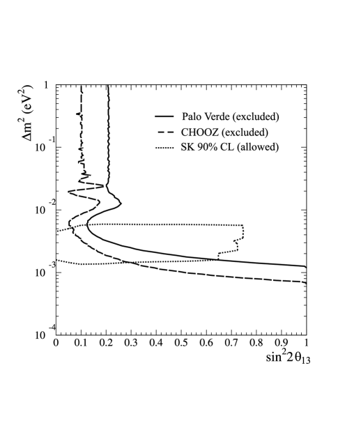
FIG. 24.: Exclusion plot showing the $allowed$ region of $\theta_{13}$ and $\Delta m^{2}$ based on the Super-Kamiokande preliminary analysis (the region $inside$ the dotted curve). The region $excluded$ by the neutrino reactor experiments are to the right of the corresponding dashed and continuous curves.

The most general approach would involve five unknown parameters, three mixing angles and two independent mass differences. However, an intermediate approach consists of a simple generalization of the two flavor scenario, assuming that $m_{3}^{2}\gg m_{1}^{2},m_{2}^{2}$ (i.e. $\Delta m_{13}^{2}=\Delta m_{23}^{2}=\Delta m^{2}$, while $\Delta m_{12}^{2}\simeq 0$). In such a case the mixing angle $\theta_{12}$ becomes irrelevant and one is left with only three unknown quantities: $\Delta m^{2},\theta_{13},{\rm and}~{}\theta_{23}$. With this parameterization the $\bar{\nu}_{e}$ disappearance is governed by

$$P(\bar{\nu}_{e}\rightarrow\bar{\nu}_{x})=\sin^{2}2\theta_{13}\sin^{2}\frac{\Delta m^{2}L}{4E_{\nu}}~{},$$ (15)

while the $\nu_{\mu}\rightarrow\nu_{\tau}$ oscillations in this scenario responsible for the atmospheric neutrino results, are described by

$$P(\nu_{\mu}\rightarrow\nu_{\tau})=\cos^{4}\theta_{13}\sin^{2}2\theta_{23}\sin^{2}\frac{\Delta m^{2}L}{4E_{\nu}}~{}.$$ (16)

A preliminary analysis of the atmospheric neutrino data based on these assumptions has been performed [28] and its results are shown in Fig. 24 for the $\bar{\nu}_{e}$ disappearance channel. One can see that while the relevant region of the mass difference $\Delta m^{2}$ is determined by the atmospheric neutrino data, the mixing angle $\theta_{13}$ is not constrained very much. Here the reactor neutrino results play a decisive role.

We plan to continue taking data through Summer of 2000, which will provide two additional reduced flux refueling periods.

REFERENCES

- [1] Y. Fukuda et al., Phys. Lett. B 335, 237 (1994).
- [2] R. Becker-Szendy et al., Phys. Rev. Lett. 69, 1010 (1992).
- [3] E. Peterson et al., Nucl. Phys. Proc. Suppl. 77, 111 (1999).
- [4] F. Boehm and P. Vogel, Physics of Massive Neutrinos, Cambridge University Press 1992 (2nd ed).
- [5] G. Zacek et al., Phys. Rev. D 34, 2621 (1986).
- [6] Y. Declais et al., Nucl. Phys. B 434, 503 (1995); and references therein.
- [7] M. Apollonio et al., Phys. Lett. B 466, 415 (1999); M. Apollonio et al., Phys. Lett. B 420, 397 (1998).
- [8] Y. Fukuda et al., Phys. Rev. Lett. 81, 1562 (1998)
- [9] F. Boehm et al., hep-ex/9912050, Phys. Rev. Lett., accepted for publication.
- [10] Model 9372 Electron Tubes Inc., Ruislip, UK.
- [11] A. G. Piepke, S. W. Moser and V. M. Novikov, Nucl. Instrum. Meth. A 432, 392 (1999).
- [12] S. P. Ahlen et al., Nucl. Instrum. Meth. A 324, 337 (1993).
- [13] G. Gratta et al., Nucl. Instrum. Meth. A 400, 456 (1997).
- [14] A. A. Hahn et al., Phys. Lett. B 218, 365 (1989).
- [15] K. Schreckenbach et al., Phys. Lett. B 160, 325 (1985).
- [16] P. Vogel et al., Phys. Rev. C 24, 1543 (1981).
- [17] P. Vogel and J. F. Beacom, Phys. Rev. D 60, 053003 (1999).
- [18] L.V. Groshev et al., Nucl. Data Tables A 5, 1. (1968).
- [19] R. Brun et al., “GEANT 3”, CERN DD/EE/84-1 (revised), 1987.
- [20] P.A. Aarnio et al., “FLUKA user’s guide”, TIS-RP-190, CERN, 1990
- [21] T.A. Gabriel et al., ORNL/TM-5619-mc, April 1977.
- [22] R.L. Craun and D.L. Smith, Nucl. Instrum. Meth. 80, 239 (1970).
- [23] G. Zacek, PhD thesis, Technical University Munich, 1984.
- [24] M. Apollonio et al., Phys. Rev. D 61, 012001 (2000).
- [25] G. J. Feldman and R. D. Cousins, Phys. Rev. D 57, 3873 (1998).
- [26] Y.F. Wang et al., hep-ex/0002050, submitted to Phys. Rev. D.
- [27] Y. Declais et al., Phys. Lett. B 338, 383 (1994).
- [28] Preliminary result, SuperKamiokande Collaboration, see also K. Okumura, Ph.D. Thesis, University of Tokyo (1999), unpublished.