Study of the Decays $B^{0}\to D^{(*)+}D^{(*)-}$

Abstract

The decays $B^{0}\to D^{*+}D^{*-}$, $B^{0}\to D^{*\pm}D^{\mp}$ and $B^{0}\to D^{+}D^{-}$ are studied in $9.7\times 10^{6}$ $\mbox{$\Upsilon(4{\rm S})$}\to\mbox{$B\bar{B}$}$ decays accumulated with the CLEO detector. We determine $\mbox{${\cal B}$}(\mbox{$B^{0}\to D^{*+}D^{*-}$})=(\mbox{$9.9{}^{+4.2}_{-3.3}\ {\rm[stat.]}\pm 1.2\ {\rm[syst.]}$})\mbox{$\times 10^{-4}$}$ and limit $\mbox{${\cal B}$}(\mbox{$B^{0}\to D^{*\pm}D^{\mp}$})<\mbox{$6.3$}\mbox{$\times 10^{-4}$}$ and $\mbox{${\cal B}$}(\mbox{$B^{0}\to D^{+}D^{-}$})<\mbox{$9.4$}\mbox{$\times 10^{-4}$}$ at 90% confidence level (CL). We also perform the first angular analysis of the $B^{0}\to D^{*+}D^{*-}$ decay and determine that the $CP$-even fraction of the final state is greater than $0.11$ at 90% CL. Future measurements of the time dependence of these decays may be useful for the investigation of $CP$ violation in neutral $B$ meson decays.

I Introduction

The first observation of $CP$ violation outside the neutral kaon system [1, 2] may well be a non-zero difference in the rates of $B^{0}\to\mbox{$J/\psi\mbox{$K^{0}_{\rm S}$}$}$ and $\bar{B}^{0}\to\mbox{$J/\psi\mbox{$K^{0}_{\rm S}$}$}$ decays [3]. Such a measurement would be an important test of the Standard Model mechanism for $CP$ violation as described by the CKM quark-mixing matrix [4]. In the Standard Model, the CKM matrix is unitary; for three quark generations, this property can be represented as a triangle in the complex plane with internal angles $\alpha$, $\beta$ and $\gamma$ [5]. Asymmetries in the rate of neutral $B$ meson decays to $CP$ eigenstates that occur via the Cabibbo-favored $\bar{b}\to\bar{c}W^{+};W^{+}\to c\bar{s}$ (eg., $B^{0}\to\mbox{$J/\psi\mbox{$K^{0}_{\rm S}$}$}$) process are expected to be proportional to $\sin 2\beta$. In contrast to the decay $B^{0}\to\mbox{$J/\psi\mbox{$K^{0}_{\rm S}$}$}$, for the Cabibbo-suppressed processes  $B^{0}\to D^{(*)+}D^{(*)-}$, the weak phase difference between the tree ($\bar{b}\to\bar{c}c\bar{d}$) and penguin ($\bar{b}\to\bar{d}c\bar{c}$) amplitudes may be appreciable [6, 7]. In the absence of a strong interaction phase difference between the tree and penguin $B^{0}\to D^{(*)+}D^{(*)-}$ amplitudes, the magnitude of the asymmetry would be also proportional to $\sin 2\beta$. The decay rate asymmetry of $B^{0}\to D^{*+}D^{*-}$ decays would also be proportional to $\sin 2\beta$ but may suffer from dilution due to the $P$-wave ($CP$-odd) component of the $D^{*+}$$D^{*-}$ final state [8, 9]. The relative $CP$-even and $CP$-odd components of the $B^{0}\to D^{*+}D^{*-}$ decay can be determined by an angular analysis [10] that removes any such dilution.

Measurements of rate asymmetries in the decays $B^{0}\to D^{(*)+}D^{(*)-}$ may provide a means to resolve the four-fold ambiguity in $\beta$ inherent in a measurement of $\sin 2\beta$ from $B^{0}\to\mbox{$J/\psi\mbox{$K^{0}_{\rm S}$}$}$ decays [8, 11, 12]. Comparison of the measured asymmetries in $B^{0}\to\mbox{$J/\psi\mbox{$K^{0}_{\rm S}$}$}$ and $B^{0}\to D^{+}D^{-}$ decays may allow partial resolution of the ambiguity in the determination of $\beta$ if the sign of the ratio of the tree and penguin amplitudes of $B^{0}\to D^{+}D^{-}$ decays can be ascertained [13]. $B^{0}$ and $\bar{B}^{0}$ mesons decay to the same $D^{*+}D^{-}$ final state with amplitudes of comparable magnitude and significant interference between them is possible [14, 15]. As for $B^{0}\to D^{+}D^{-}$, the asymmetry between the rates of $\mbox{$B^{0}$}\to D^{*+}D^{-}$ and $\mbox{$\bar{B}^{0}$}\to D^{*-}D^{+}$ is directly proportional to $\sin 2\beta$ in the absence of strong phase differences. In the presence of a strong phase difference, the rate asymmetry would depend on both $\sin 2\beta$ and $\cos 2\beta$ and, when combined with a $\sin 2\beta$ measurement from $B^{0}\to\mbox{$J/\psi\mbox{$K^{0}_{\rm S}$}$}$ decays, could aid in the resolution of ambiguities in the determination of $\beta$.

The decay $B^{0}\to D^{*\pm}D^{\mp}$ would also provide a clean test of the factorization ansatz for decays into two charm mesons and provide a measurement of the ratio of $D^{*+}$ and $D^{+}$ decay constants and form factors [9, 14].

The expected branching fractions of the decays $B^{0}\to D^{(*)+}D^{(*)-}$ can be estimated from the measurement of the corresponding Cabibbo-favored processes $B^{0}\to D^{(*)+}_{s}D^{(*)-}$ [5] and the ratio of decay constants [8, 16]. The estimated $B^{0}\to D^{*+}D^{*-}$ branching fraction is $\sim 10\mbox{$\times 10^{-4}$}$, consistent with the measurement of $(6.2{}^{+4.0}_{-2.9}\ {\rm[stat.]}\pm 1.0\ {\rm[syst.]})\mbox{$\times 10^{-4}$}$ [17], and the estimates for $B^{0}\to D^{*\pm}D^{\mp}$ and $B^{0}\to D^{+}D^{-}$ are $\sim 8\mbox{$\times 10^{-4}$}$ and $\sim 5\mbox{$\times 10^{-4}$}$, respectively.

We present an update of the previous CLEO measurement of ${\cal B}$($B^{0}\to D^{*+}D^{*-}$) [17] and improved upper limits on ${\cal B}$($B^{0}\to D^{*\pm}D^{\mp}$) and ${\cal B}$($B^{0}\to D^{+}D^{-}$) [18] based upon a sample of $9.7\times 10^{6}$ $B\bar{B}$ pairs produced in $e^{+}e^{-}$$\to$$\Upsilon(4{\rm S})$ decays accumulated with the CLEO detector at the Cornell Electron Storage Ring (CESR). We also present the first angular analysis of $B^{0}\to D^{*+}D^{*-}$ decays and limit the $CP$-odd content of this reaction. The results presented here supersede the previous CLEO results [17, 18].

II The CLEO detector

The data were accumulated with two configurations of the CLEO detector dubbed CLEO II [19] and CLEO II.V [20]. In the first configuration, a 1.5T solenoidal magnetic field encloses three concentric cylindrical drift chambers that are nested within a cylindrical barrel of time-of-flight (TOF) scintillators and a CsI(Tl) calorimeter. The surrounding iron return yoke is instrumented with proportional wire chambers for muon identification. The large outer drift chamber provides up to 49 measurements of a charged particle’s specific ionization ($dE/dx$) for particle species identification. In the CLEO II.V configuration, the innermost wire chamber was replaced by a three-layer, silicon vertex detector (SVX) capable of providing precision position information in both $r\phi$ and $z$ [21]. The gas in the large outer drift chamber was also changed from argon-ethane to helium-propane, resulting in improved $dE/dx$ and momentum resolution [22].

The Monte Carlo simulation of the CLEO detector response was based upon GEANT [23]. Simulated events for the CLEO II and CLEO II.V configurations were processed in the same manner as the data.

III Charm meson reconstruction

Observation of the relatively small rates expected for $B^{0}\to D^{(*)+}D^{(*)-}$ decays requires an aggressive program of charm meson reconstruction. The $D^{0}$ decay modes considered for reconstruction are ${K^{-}}\pi^{+}$, ${K^{-}}\pi^{+}\pi^{0}$, ${K^{-}}\pi^{+}\pi^{+}\pi^{-}$, ${K}^{0}_{\rm S}\pi^{+}\pi^{-}$ and ${K}^{0}_{\rm S}\pi^{+}\pi^{-}\pi^{0}$; the $D^{+}$ decay modes considered for reconstruction are ${K^{-}}\pi^{+}\pi^{+}$, ${K}^{0}_{\rm S}\pi^{+}$, ${K}^{0}_{\rm S}\pi^{+}\pi^{0}$, ${K}^{0}_{\rm S}\pi^{+}\pi^{+}\pi^{-}$, ${K^{-}}\pi^{+}\pi^{+}\pi^{0}$, ${K^{-}K^{+}}\pi^{+}$ and ${K^{-}K^{+}}\pi^{+}\pi^{0}$. In order to limit background, the decay $\mbox{$D^{+}$}\to\mbox{${K^{-}}\pi^{+}\pi^{+}\pi^{0}$}$ is not considered for the reconstruction of the $B^{0}\to D^{*+}D^{*-}$ mode and the decays $\mbox{$D^{+}$}\to\mbox{${K^{-}K^{+}}\pi^{+}$}$ and $\mbox{$D^{+}$}\to\mbox{${K^{-}K^{+}}\pi^{+}\pi^{0}$}$ are not considered for the reconstruction of the $B^{0}\to D^{+}D^{-}$ mode. The $D^{*+}$ decays to $\mbox{$D^{0}$}\pi^{+}$ and $\mbox{$D^{+}$}\pi^{0}$ are selected for the reconstruction of the $B^{0}\to D^{*+}D^{*-}$ and $B^{0}\to D^{*\pm}D^{\mp}$ modes, although the final state $(D^{+}\pi^{0})(D^{-}\pi^{0})$ is overwhelmed by combinatorial background and is excluded from the $B^{0}\to D^{*+}D^{*-}$ reconstruction. In the following, “$D$” refers to either $D^{+}$ or $D^{0}$ mesons, “$\pi_{\rm s}$” refers to the slow pion daughter of the $D^{*+}$ decay and charge conjugation is implied unless explicitly stated otherwise.

Charged kaon and pion daughters of $D$ meson candidates must be compatible with an origin at the $e^{+}e^{-}$ interaction point. The $dE/dx$ or TOF measurement of a charged track, when available, must be within 2.5 and 3.0 standard deviations ($\sigma$) of expectations for $K^{\pm}$ and $\pi^{\pm}$ candidates, respectively. The $K^{0}_{\rm S}$ meson candidates are reconstructed in the $\pi^{-}\pi^{+}$ decay mode and must be consistent with an origin at the $e^{+}e^{-}$ interaction point. At least one of the $K^{0}_{\rm S}$ daughter pions must be inconsistent with an origin at the $e^{+}e^{-}$ interaction point. Neutral pion candidates are formed from energy deposits in the calorimeter consistent with electromagnetic showers unassociated with a charged track and with an energy exceeding 30 MeV in the barrel ($|\cos\theta|<0.71$) and 50 MeV in the endcap region where $\theta$ is the angle of the shower with respect to the $z$ axis. A requirement on the $\pi^{0}$ minimumn momentum of 100 MeV/$c$ is imposed for $D$ daughter candidates and of 70 MeV/$c$ for $D^{*+}$ daughter candidates. The charged and $K^{0}_{\rm S}$ daughters of all $D$ meson candidates are required to originate from a common vertex.

IV $B^{0}$ meson candidate selection

A number of observables are used to suppress backgrounds. In general, the requirements on these are more stringent for the $B^{0}\to D^{*\pm}D^{\mp}$ and $B^{0}\to D^{+}D^{-}$ modes than for $B^{0}\to D^{*+}D^{*-}$ because the combinatorial backgrounds are larger. In addition, while common selection criteria for all $D^{*+}$ and $D$ decay modes of each $B^{0}$ candidate were satisfactory for the $B^{0}\to D^{*+}D^{*-}$ mode, the $B^{0}\to D^{*\pm}D^{\mp}$ and $B^{0}\to D^{+}D^{-}$ modes require separate criteria for each $B^{0}\to D^{(*)+}D^{-}$ channel  to reduce background. The selection criteria for each channel of the $B^{0}\to D^{*\pm}D^{\mp}$ and $B^{0}\to D^{+}D^{-}$ modes were optimized using simulated signal and background events assuming $\mbox{${\cal B}$}(\mbox{$B^{0}\to D^{*\pm}D^{\mp}$})=8\mbox{$\times 10^{-4}$}$ and $\mbox{${\cal B}$}(\mbox{$B^{0}\to D^{+}D^{-}$})=4.5\mbox{$\times 10^{-4}$}$, respectively.

A $B^{0}$ meson candidate energy and mass

The observable $\mbox{$\Delta E$}\equiv E(D^{(*)+})+E(D^{(*)-})-E_{\rm beam}$ exploits energy conservation for $B^{0}$$\bar{B}^{0}$ meson pairs produced in $\Upsilon(4{\rm S})$ decays and has a resolution $\sigma(\mbox{$\Delta E$})=8\ {\rm MeV}$ after constraining the $B^{0}$ daughter candidates to the $D^{(*)+}$ masses [5]. The beam-constrained $B$ mass is defined as $\mbox{$M(B)$}^{2}\equiv E^{2}_{\rm beam}-{{\bf p}}_{B}^{2}$, where ${{\bf p}}_{B}$ is the measured $B^{0}$ candidate momentum. The $M(B)$ resolution of 2.5 MeV is dominated by the beam energy spread [24]. Signal candidates are selected by requiring both $\Delta E$ and $\mbox{$M(B)$}-M^{\rm n}_{B}$ to be within $2.5\sigma$ of zero for the $B^{0}\to D^{*+}D^{*-}$ mode and within $2.0\sigma$ of zero for the $B^{0}\to D^{*\pm}D^{\mp}$ and $B^{0}\to D^{+}D^{-}$ modes, where $M^{\rm n}_{B}$ is the world-average $B^{0}$ mass [5].

B Candidate mass $\chi^{2}$

The overall deviation of $D^{*+}$ and $D$ candidates from the $D^{*+}$ and $D$ meson masses is quantified by

$$\mbox{$\chi^{2}_{M}$}\equiv\sum_{i}\left(\frac{M_{i}-M_{i}^{\rm n}}{\sigma(M_{i})}\right)^{2}+\left(\frac{\Delta M_{i}-\Delta M_{i}^{\rm n}}{\sigma(\Delta M_{i})}\right)^{2}\ \ \ ,$$ (1)

where $M_{i}$ is the measured $D$ candidate mass, $\Delta M_{i}$ is the mass difference between the $D^{*+}$ and $D$ candidates, and $\sigma(M_{i})$ and $\sigma(\Delta M_{i})$ are the corresponding resolutions. The superscript “n” denotes the world-average mass or mass difference [5]. The sum runs over $i=D^{(*)+},D^{(*)-}$; the second term in Eqn. (1) is not present for $B^{0}\to D^{+}D^{-}$ candidates and is only present for the $i=\mbox{$D^{*+}$}$ term for $B^{0}\to D^{*\pm}D^{\mp}$ candidates. For $B^{0}\to D^{*+}D^{*-}$ candidates, the average resolutions were used; for $B^{0}\to D^{*\pm}D^{\mp}$ and $B^{0}\to D^{+}D^{-}$ decays, the resolution for each $D$ and $D^{*+}$ candidate was determined from the track covariance matrices. If more than one $B^{0}\to D^{(*)+}D^{(*)-}$ candidate was present in a single event after all other selection criteria were applied, the one with the smallest $\chi^{2}_{M}$ was selected. This observable is most effective for $B^{0}\to D^{*+}D^{*-}$ since $\sigma(\Delta M)\approx 500\ {\rm keV}$ and $350\ {\rm keV}$ for the $\mbox{$D^{0}$}\pi^{+}$ final state in CLEO II and CLEO II.V, respectively. We require $\mbox{$\chi^{2}_{M}$}<10$ for $B^{0}\to D^{*+}D^{*-}$ candidates [17]. A typical requirement on $\chi^{2}_{M}$ is $<\!6$ for $B^{0}\to D^{*\pm}D^{\mp}$($\mbox{$D^{*+}$}\to\mbox{$D^{0}$}\pi^{+},\,\mbox{$D^{0}$}\to\mbox{${K^{-}}\pi^{+}\pi^{0}$},\,\mbox{$D^{-}$}\to\mbox{${K^{+}}\pi^{-}\pi^{-}$}$) and $<\!4$ for $B^{0}\to D^{+}D^{-}$($\mbox{$D^{+}$}\to\mbox{${K^{-}}\pi^{+}\pi^{+}$},\,\mbox{$D^{-}$}\to\mbox{${K^{+}}\pi^{-}\pi^{-}$}$).

C Separation between the $D$ and $\bar{D}$ decay vertices

The observable $L/\sigma(L)$ exploits the relatively long decay length of the $D^{+}$ meson ($\gamma\beta c\tau\approx 250\ \mu{\rm m}$) and is defined as

$$L\equiv({{\bf v}}_{D}-{{\bf v}}_{\bar{D}})\cdot\frac{({{\bf p}}_{D}-{{\bf p}}_{\bar{D}})}{|{{\bf p}}_{D}-{{\bf p}}_{\bar{D}}|}\ \ ,$$ (2)

where ${{\bf v}}_{D}$ (${{\bf p}}_{D}$) is the reconstructed $D$ candidate decay vertex (momentum). The resolution $\sigma(L)$ is determined from the $D$ candidates’ covariance matrices; typically, $\sigma(L)=500\ (200)\ \mu{\rm m}$ for CLEO II (CLEO II.V). For CLEO II, only the 2-dimensional $r\phi$ information is precise enough to provide some discrimination so we use only the $r\phi$ projection of $L$; in CLEO II.V, the SVX allows the use of the full 3-dimensional vertex information. We require $\mbox{$L/\sigma(L)$}>0$ for $\mbox{$B^{0}\to D^{*+}D^{*-}$}\to(\mbox{$D^{+}$}\pi^{0})(\bar{D}^{0}\pi^{-})$ candidates in CLEO II.V only [17]. For the CLEO II.V detector configuration, typical requirements on $L/\sigma(L)$ are $>-0.5$ for $B^{0}\to D^{*\pm}D^{\mp}$($\mbox{$D^{*+}$}\to\mbox{$D^{0}$}\pi^{+},\,\mbox{$D^{0}$}\to\mbox{${K^{-}}\pi^{+}\pi^{0}$},\,\mbox{$D^{-}$}\to\mbox{${K^{+}}\pi^{-}\pi^{-}$}$) and $\mbox{$L/\sigma(L)$}>2.5$ for $B^{0}\to D^{+}D^{-}$($\mbox{$D^{+}$}\to\mbox{${K^{-}}\pi^{+}\pi^{+}$},\,\mbox{$D^{-}$}\to\mbox{${K^{+}}\pi^{-}\pi^{-}$}$).

D Thrust and helicity angle

For the $B^{0}\to D^{*\pm}D^{\mp}$ and $B^{0}\to D^{+}D^{-}$ modes, the observable $\cos\mbox{$\theta_{\rm T}$}$ was used to suppress non-$B\bar{B}$ background. The angle between the thrust axis [25] of the $B^{0}$ candidate and the thrust axis of the remainder of the event is $\theta_{\rm T}$. Continuum ($\mbox{$e^{+}e^{-}$}\to\mbox{$q\bar{q}$}$, $q=u,c,s,d$) backgrounds are sharply peaked towards $|\mbox{$\cos\mbox{$\theta_{\rm T}$}$}|=1$ and signal events are uniform in $\cos\mbox{$\theta_{\rm T}$}$. The maximum allowed $|\mbox{$\cos\mbox{$\theta_{\rm T}$}$}|$ ranges from 0.50 to 0.95 for the $B^{0}\to D^{*\pm}D^{\mp}$ channels and from 0.80 to 0.95 for the $B^{0}\to D^{+}D^{-}$ channels.

The ${\rm pseudoscalar}\to{\rm vector},{\rm pseudoscalar}$ decay $B^{0}\to D^{*\pm}D^{\mp}$ produces a $\cos^{2}\mbox{$\theta_{\rm H}$}$ distribution for signal and is uniform for background. The angle $\theta_{\rm H}$ is taken between the $\pi_{\rm s}$ and the $D^{*+}$ in the $D^{*+}$ rest frame. The minimum allowed $|\mbox{$\cos\mbox{$\theta_{\rm H}$}$}|$ for $B^{0}\to D^{*\pm}D^{\mp}$ candidates lies in the range $0.1$ to $0.7$, depending on the decay channel.

E $D^{+}$ decay length

The $B^{0}\to D^{+}D^{-}$ mode suffers from a background that consists of a $D^{+}$ candidate where the majority of daughter candidate tracks are the result of a $D^{+}$ meson decay and a $D^{-}$ candidate composed of a random combination of tracks. The observable $L/\sigma(L)$ (Sec. IV C) does not sufficiently suppress this background due to the decay length of the $D^{+}$ candidate, but a requirement on $S\equiv\min(d_{D}/\sigma(d_{D}),d_{\bar{D}}/\sigma(d_{\bar{D}}))$, the minimum decay length significance of the $B^{0}$ daughters, where $d_{D}\equiv({{\bf v}}_{D}-{{\bf v}}_{B})\cdot{{\bf p}}_{D}/|{{\bf p}}_{D}|$, reduces this background component. The average $B^{0}$ decay length is $\sim 30\ \mu{\rm m}$; therefore, the $B^{0}$ decay vertex ${{\bf v}}_{B}$ can be accurately approximated as the $e^{+}e^{-}$ interaction point. For the ${K^{-}}\pi^{+}\pi^{+}$, ${K^{+}}\pi^{-}\pi^{-}$ final state, we require $S>-0.5$ for the CLEO II.V configuration.

For the $B^{0}\to D^{*\pm}D^{\mp}$ and $B^{0}\to D^{+}D^{-}$ modes, there are channels for which the background could not be reduced to a reasonable level with any combination of selection criteria. Specific $B^{0}\to D^{*\pm}D^{\mp}$ channels were discarded if the background estimated from simulation could not be reduced below $1/6$ of the expected signal rate. Out of 84 possible channels considered, a total of 57 and 67 $B^{0}\to D^{*\pm}D^{\mp}$ channels survive this criterion for the CLEO II and CLEO II.V detector configurations, respectively. Similarly, $B^{0}\to D^{+}D^{-}$ channels for which the background could not be reduced below $1/3$ or $1/7$ of the expected signal rate for the CLEO II or CLEO II.V configuration, respectively, were rejected. These criteria select 8 and 7 out of a total of 15 possible $B^{0}\to D^{+}D^{-}$ channels for the CLEO II and CLEO II.V configurations, respectively.

V Results and interpretation

The $\Delta E$ versus $M(B)$ distributions of $B^{0}\to D^{*+}D^{*-}$, $B^{0}\to D^{*\pm}D^{\mp}$ and $B^{0}\to D^{+}D^{-}$ candidates passing all selection criteria are shown in Figures 1, 2 and 3, respectively. A significant signal is apparent for $B^{0}\to D^{*+}D^{*-}$ decays; the larger backgrounds for the $B^{0}\to D^{*\pm}D^{\mp}$ and $B^{0}\to D^{+}D^{-}$ modes are discussed below.

A Background estimation

For all three modes, the background is estimated with two independent methods based on samples drawn largely from the data [17]. Method 1 uses the grand sideband (GSB) indicated in Figures 1, 2 and 3. The observed number of candidates in the GSB in each channel is scaled to estimate the background in the signal region. The scale factors are $(7.3\pm 2.2)\mbox{$\times 10^{-3}$}$, $(4.7\pm 1.2)\mbox{$\times 10^{-3}$}$, $(4.3\pm 0.7)\mbox{$\times 10^{-3}$}$ and $(4.0\pm 0.9)\mbox{$\times 10^{-3}$}$ for the $B^{0}\to D^{*+}D^{*-}$, $B^{0}\to D^{*\pm}D^{\mp}$(CLEO II), $B^{0}\to D^{*\pm}D^{\mp}$(CLEO II.V) and $B^{0}\to D^{+}D^{-}$ analyses, respectively, and are estimated from the fitted distributions in $M(B)$ and $\Delta E$. The excluded region of the GSB contains fully- or partially-reconstructed $B\to D^{(*)+}D^{(*)-}X$ decays that cannot enter the signal region. The GSB regions are slightly smaller for the $B^{0}\to D^{(*)+}D^{-}$ analyses because they suffer from “reflection” background. “Reflection” backgrounds arise if Cabibbo-favored $B^{0}\to D^{(*)+}_{s}D^{(*)-}$ decays are interpreted as $B^{0}\to D^{(*)+}D^{-}$ when a charged kaon from the $D_{s}^{(*)+}$ is misidentified as a pion. This background has $\mbox{$\Delta E$}\leq-50\ {\rm MeV}$ due to the kinematics of the $D_{s}^{+}$ decay combined with the difficulty in distinguishing $K^{\pm}$ from $\pi^{\pm}$ for $|{{\bf p}}|\geq 800\ {\rm MeV}/c$ with $dE/dx$ or TOF.

For method 2 the contribution of each background component was estimated separately. The dominant contribution to the background consists of combinations of $D^{(*)+}$ and $D^{(*)-}$ in which one or both candidates is fake; that is, the $D^{(*)}$ daughter candidates are not the result of a $D^{(*)}$ meson decay. This combinatorial background can be estimated by forming explicit fake $D^{(*)+}$ candidates drawn from the $D$ candidate mass sidebands by replacing $M_{i}^{\rm n}$ in Eqn. 1 with $M_{i}^{\rm n}+f\sigma(M_{i})$ or $M_{i}^{\rm n}-f\sigma(M_{i})$. We use $f=6$ so that classification of each $D$ meson candidate as fake or standard is unique given the $\chi^{2}_{M}$ selection criteria. The contribution to each channel of the combinatorial background can be derived from the two samples consisting of fake $D^{(*)+}$ and standard $D^{(*)-}$ candidates or fake $D^{(*)+}$ and fake $D^{(*)-}$ candidates.

Two other background components are due to random combinations of real $D^{(*)+}$ and $D^{(*)-}$ mesons that are approximately back-to-back and arise from the processes $\mbox{$e^{+}e^{-}$}\to\mbox{$c\bar{c}$}\to\mbox{$D^{(*)+}$}\mbox{$D^{(*)-}$}\ X$ or $\mbox{$e^{+}e^{-}$}\to\mbox{$\Upsilon(4{\rm S})$}\to\mbox{$B\bar{B}$}\to(\mbox{$D^{(*)+}$}X)(\mbox{$D^{(*)-}$}Y)$. The $\mbox{$e^{+}e^{-}$}\to\mbox{$c\bar{c}$}\to\mbox{$D^{(*)+}$}\mbox{$D^{(*)-}$}\ X$ component was estimated from $4.6\ {\rm fb}^{-1}$ of $e^{+}e^{-}$ data taken 60 MeV below the $\Upsilon(4{\rm S})$ resonance after subtraction of the combinatorial background using the method described above. The $\mbox{$e^{+}e^{-}$}\to\mbox{$\Upsilon(4{\rm S})$}\to\mbox{$B\bar{B}$}\to(\mbox{$D^{(*)+}$}X)(\mbox{$D^{(*)-}$}Y)$ component was estimated from samples of simulated events at least 10 times the data sample size. The estimated total backgrounds are listed in Table I. The estimates from the two methods for each channel are in good agreement and are combined channel-by-channel to produce the overall background estimate.

TABLE I.: Background estimates. The two background estimation methods are described in the text. For method 2, the combinatorial, $c\bar{c}$ and $B\bar{B}$ components of the background are listed separately. The uncertainties in the table are statistical only and do not include the uncertainty due to the background scaling factor derived from the fitted $\Delta E$ and $M(B)$ distributions (Sec. V A).

	Method 1	Method 2
Decay	Total	Total	combinatorial	$c\bar{c}$	$B\bar{B}$
$B^{0}\to D^{*+}D^{*-}$	$0.384\pm 0.053$	$0.469\pm 0.057$	$0.382\pm 0.046$	$0.052\pm 0.034$	$0.035\pm 0.005$
$B^{0}\to D^{*\pm}D^{\mp}$	$1.874\pm 0.102$	$1.795\pm 0.098$	$1.336\pm 0.062$	$0.305\pm 0.078$	$0.064\pm 0.005$
$B^{0}\to D^{+}D^{-}$	$0.498\pm 0.048$	$0.459\pm 0.041$	$0.433\pm 0.039$	$0.014\pm 0.003$	$0.013\pm 0.003$

We assess the probability for the estimated background to produce a more “signal-like” configuration of candidates than the observed $B\to\mbox{$D^{(*)+}$}\mbox{$D^{-}$}$ signal candidates with the likelihood ${\cal L}=\prod_{i}f(b_{i};n_{i})$, where the product runs over all channels selected for either the $B^{0}\to D^{*\pm}D^{\mp}$ or $B^{0}\to D^{+}D^{-}$ analysis, $f(\mu;n)\equiv e^{-\mu}\mu^{n}/n!$, $b_{i}$ is the estimated background in the $i^{\rm th}$ channel and $n_{i}$ is the observed number of signal candidates in the $i^{\rm th}$ channel. We compare the distribution of ${\cal L}$ for many simulated experiments consisting solely of background with the value of ${\cal L}$ obtained for the signal candidates in the data. In the simulation of the background-only experiments, we take into account both the statistical and systematic uncertainty in the per-channel background estimates. For the $B^{0}\to D^{*\pm}D^{\mp}$ and $B^{0}\to D^{+}D^{-}$ mode, a total of $0.3\%$ and $3.8\%$, respectively, of the simulated, background-only experiments had ${\cal L}>{\cal L}_{\rm data}$ and, hence, are more signal-like than the observed candidates. These rates are too large to claim an unambiguous observation of either the $B^{0}\to D^{*\pm}D^{\mp}$ or $B^{0}\to D^{+}D^{-}$mode. For the $B^{0}\to D^{*+}D^{*-}$ mode, fewer than $2\times 10^{-7}$ background-only experiments were more signal-like than the data.

B Branching fraction determination

The $B^{0}\to D^{(*)+}D^{(*)-}$ branching fractions are determined from the likelihood

$${\cal L}(\mbox{${\cal B}$})=\prod_{i}f(\mu_{i};n_{i})\ \ ,$$ (3)

where

• $\mbox{${\cal B}$}\equiv\mbox{${\cal B}$}(\mbox{$B^{0}\to D^{(*)+}D^{(*)-}$})$,

• $\mu_{i}=s_{i}+b_{i}$,

• $s_{i}=2f_{00}N(\mbox{$B\bar{B}$})\epsilon_{i}\mbox{${\cal B}$}_{i}(\mbox{$D^{(*)+}$})\mbox{${\cal B}$}(\mbox{$B^{0}\to D^{(*)+}D^{(*)-}$})$,

• $\epsilon_{i}$ is the reconstruction efficiency of the $i^{\rm th}$ channel,

• $\mbox{${\cal B}$}_{i}(\mbox{$D^{(*)+}$})$ is the product daughter branching fractions of the $i^{\rm th}$ channel and

• $N(\mbox{$B\bar{B}$})$ is the number of $B\bar{B}$ pairs.

We assume $f_{00}/f_{+-}\equiv\mbox{${\cal B}$}(\mbox{$\Upsilon(4{\rm S})$}\to\mbox{$B^{0}$}\bar{B}^{0})/\mbox{${\cal B}$}(\mbox{$\Upsilon(4{\rm S})$}\to B^{+}B^{-})=1$ for the results presented here. The evaluation of ${\cal L}(\mbox{${\cal B}$})$ takes into account the systematic uncertainties due to the background estimate, efficiencies and $D^{(*)+}$ daughter branching fractions [5]. The branching fractions and upper limits at 90% CL for the three $B^{0}$ decay modes are listed in Table II. Since the background estimates of the two methods are combined channel-by-channel, the combination of the total background estimates of methods 1 and 2 (Table I) differs slightly from the total background estimate given in Table II. Furthermore, the evaluation of the $B^{0}\to D^{(*)+}D^{(*)-}$ branching fractions with a likelihood function that takes into account the reconstruction efficiency, daughter branching fractions and backgrounds of each channel (Eqn. (3)) differs from the branching fraction that would be derived from the average efficiency times daughter branching fraction and total backgrounds listed in Table II.

While only the $B^{0}\to D^{*+}D^{*-}$ results provide unambiguous evidence of the Cabibbo-suppressed $\bar{b}\to\bar{c}c\bar{d}$ decay, the expectations based on the corresponding Cabibbo-favored decays are consistent with the upper limits of the other two modes. The results presented here indicate that there may be potential difficulties in the measurement of $\sin 2\beta$ using $B^{0}\to D^{(*)+}D^{(*)-}$ decays. The yields are appreciably lower than that of $B^{0}\to\mbox{$J/\psi\mbox{$K^{0}_{\rm S}$}$}$ for the same integrated luminosity, and background levels are higher, especially for $B^{0}\to D^{*\pm}D^{\mp}$ and $B^{0}\to D^{+}D^{-}$. Measurement of $\sin 2\beta$ via the proper-time dependence of $\mbox{$B^{0}$}\to\mbox{$D^{(*)+}$}\mbox{$D^{-}$}$ decays performed at asymmetric $e^{+}e^{-}$ colliders or at hadron colliders may be able to exploit the $B^{0}$ decay length to reduce backgrounds. In contrast, the $B^{0}\to D^{*+}D^{*-}$ results show that this mode, while also having a yield substantially lower than that of $B^{0}\to\mbox{$J/\psi\mbox{$K^{0}_{\rm S}$}$}$, has very low backgrounds and should provide an independent measure of $\sin 2\beta$. The suppression of background for $B^{0}\to D^{*+}D^{*-}$ is achieved largely through the observable $\chi^{2}_{M}$(Sec. IV B) that relies on accurate reconstruction of the trajectory of the charged slow pion from the $D^{*+}$ decay. Inability to reconstruct efficiently the $\pi_{\rm s}^{+}$ can substantially degrade a potential $\sin 2\beta$ measurement. For example, for the results presented here, the reconstruction efficiency of the $\pi_{\rm s}^{+}$ from $\mbox{$D^{*+}$}\to\mbox{$D^{0}$}\pi_{\rm s}^{+}$ for the CLEO II.V configuration is $(65\pm 6)\%$ of that for the CLEO II configuration because the track-finding algorithm was optimized only for the latter configuration [17].

TABLE II.: The number of observed candidates, estimated total backgrounds, efficiencies, measured branching fractions and branching fraction upper limits at 90% CL for the three $B^{0}\to D^{(*)+}D^{(*)-}$ modes. For the branching fractions and background, the first error is the statistical uncertainty and the second is the systematic uncertainty. $\langle\epsilon\mbox{${\cal B}$}\rangle$ is the product of the reconstruction efficiencies and the $D^{(*)}$ daughter branching fractions summed over all channels; the uncertainty includes both the statistical uncertainty in the estimation of $\epsilon_{i}$ from simulation as well as the uncertainties in the daughter branching fractions [5].

Decay		Total	$\langle\epsilon\mbox{${\cal B}$}\rangle$	Branching	90%CL Upper
mode	Candidates	background	($\times 10^{-4}$)	fraction ($\times 10^{-4}$)	limit ($\times 10^{-4}$)
$B^{0}\to D^{*+}D^{*-}$	8	$0.42\pm 0.04\pm 0.13$	$8.2\pm 2.9$	$9.9{}^{+4.2}_{-3.3}\pm 1.2$	—
$B^{0}\to D^{*\pm}D^{\mp}$	6	$1.68\pm 0.07\pm 0.24$	$11.0\pm 1.7$	$2.1{}^{+2.4}_{-1.7}\pm 0.5$	$6.3$
$B^{0}\to D^{+}D^{-}$	2	$0.46\pm 0.03\pm 0.10$	$5.4\pm 1.0$	$3.0{}^{+3.3+0.8}_{-2.1-0.6}$	$9.4$

C $B^{0}\to D^{*+}D^{*-}$ transversity analysis

A measurement of $\sin 2\beta$ from $B^{0}\to D^{*+}D^{*-}$ decays requires an angular analysis to disentangle the $CP$-odd and $CP$-even components of the decay. In the transversity basis [10], the fraction of the $CP$-even component ($A$) of the decay $B^{0}\to D^{*+}D^{*-}$ can be determined from the $\cos\mbox{$\theta_{tr}$}$ distribution,

$$\frac{1}{\Gamma}\frac{d\Gamma}{d\mbox{$\cos\mbox{$\theta_{tr}$}$}}=\frac{3}{4}A\sin^{2}\mbox{$\theta_{tr}$}+\frac{3}{2}(1-A)\cos^{2}\mbox{$\theta_{tr}$}\ \ \ ,$$ (4)

where $\Gamma\equiv\Gamma(\mbox{$B^{0}\to D^{*+}D^{*-}$})+\Gamma(\mbox{$\bar{B}^{0}\to D^{*+}D^{*-}$})$ and $\theta_{tr}$ is the angle between the $\pi_{\rm s}$ from the $D^{*+}$ and the normal to the plane of the $D^{*-}$ decay in the $D^{*+}$ rest frame as shown in Fig. 4.

We perform an unbinned, maximum likelihood fit to extract $A$ from the $\cos\mbox{$\theta_{tr}$}$ distribution of the eight $B^{0}\to D^{*+}D^{*-}$ candidates, taking into account the background shape and the $\cos\mbox{$\theta_{tr}$}$ resolution and acceptance. The background shape, estimated from GSB candidates, is consistent with being uniform as a function of $\cos\mbox{$\theta_{tr}$}$. The resolution of $\sigma(\mbox{$\cos\mbox{$\theta_{tr}$}$})=0.1$ is determined from simulated events in the observed decay channels. The acceptance varies as a function of $\cos\mbox{$\theta_{tr}$}$ due to the drop in efficiency at low momentum for the charged $\pi_{\rm s}$. For $\pi^{+}_{\rm s}$ emitted perpendicular (parallel) to the $D^{*+}$ direction, $\cos\mbox{$\theta_{tr}$}$ tends towards $\pm 1$ (0). Thus a loss of efficiency for low momentum $\pi^{+}_{\rm s}$ results in a reduction of acceptance at $\cos\mbox{$\theta_{tr}$}$ near zero. This effect is inconsequential for the $\mbox{$D^{*+}$}\to\mbox{$D^{+}$}\pi^{0}$ candidates because the $\pi^{0}_{\rm s}$ efficiency does not vary appreciably. The acceptance is modeled as $\propto 1+\alpha\cos^{2}\mbox{$\theta_{tr}$}$, where $\alpha=0.17\pm 0.17$ is determined from simulated $B^{0}\to D^{*+}D^{*-}$ decays and the uncertainty represents a conservative estimate of the range of $\alpha$.

The observed $\cos\mbox{$\theta_{tr}$}$ distribution of the $B^{0}\to D^{*+}D^{*-}$ candidates is shown in Fig. 5 with the fit result superimposed. Figure 6 shows the dependence of $L(A)\equiv-2\ln({\cal L}(A)/{\cal L}(\tilde{A}))$, assuming $\alpha=0.34$ where $\tilde{A}$ is the value of $A$ that maximizes ${\cal L}(A)$. The conventional evaluation of confidence levels from $L(A)$ is confounded because the statistical resolution on $A$ is comparable to the bounds on $A$ of $[0,1]$. To determine confidence levels, we evaluate $L(A)$ as a function of the input value of $A$ using 10000 simulated experiments at each value of $A_{\rm input}=0.0,0.1,0.2,\ldots,1.0$. Each simulated experiment is analyzed as the data and the distribution of $dN/dL(A_{\rm input})$ is determined ($N$ is the number of simulated experiments). At each value of $A_{\rm input}$, we then determine the 95% CL value, $L_{95}$, as

$${\int_{0}^{L_{95}}dL\,\frac{dN}{dL}}\Big{/}{\int_{0}^{\infty}dL\,\frac{dN}{dL}}=0.95\ \ \ \ .$$ (5)

In Fig. 6 we show the curves resulting from this procedure at the 68.3, 90, 95 and 99% CL for $\alpha=0.34$. The confidence level curves have a concave shape because the $dN/dL$ distributions peak more sharply at $A_{\rm input}$ near 0 and 1 due to the bounds on $A$. We perform this procedure for the central and extreme values of the acceptance, $\alpha=0.00,0.17,0.34$, for both the simulation and the data to take into account the acceptance uncertainty. We conservatively use the regions excluded by all three values of $\alpha$ to set limits. We exclude values of $A<0.11$ at 90% CL, but cannot exclude $A=0$ at 99% CL. Combining the limits $0.15<A<0.90$ at 68.3% CL for the three values of $\alpha$ with the most likely value of $A$ for $\alpha=0.17$ and taking into account the uncertainties in the level and shape of the background, we find $A=\mbox{$0.49{}^{+0.41}_{-0.34}\pm 0.02$}$. Our results are consistent with expectations that $A\approx 0.95$[8, 11, 9], although the statistical precision is poor.

VI Summary and conclusions

We have studied the decays $B^{0}\to D^{*+}D^{*-}$, $B^{0}\to D^{*\pm}D^{\mp}$ and $B^{0}\to D^{+}D^{-}$in $9.7\times 10^{6}$ $\mbox{$\Upsilon(4{\rm S})$}\to\mbox{$B\bar{B}$}$ decays. We determine $\mbox{${\cal B}$}(\mbox{$B^{0}\to D^{*+}D^{*-}$})=(\mbox{$9.9{}^{+4.2}_{-3.3}\ {\rm[stat.]}\pm 1.2\ {\rm[syst.]}$})\mbox{$\times 10^{-4}$}$ and limit $\mbox{${\cal B}$}(\mbox{$B^{0}\to D^{*\pm}D^{\mp}$})<\mbox{$6.3$}\mbox{$\times 10^{-4}$}$ and $\mbox{${\cal B}$}(\mbox{$B^{0}\to D^{+}D^{-}$})<\mbox{$9.4$}\mbox{$\times 10^{-4}$}$ at 90% CL. These results, while consistent with expectations, show that substantially higher luminosities will be needed to make a measurement of $\sin 2\beta$ using $B^{0}\to D^{(*)+}D^{(*)-}$ decays that approaches the statistical precision of a $\sin 2\beta$ measurement using $B^{0}\to\mbox{$J/\psi\mbox{$K^{0}_{\rm S}$}$}$. Asymmetry measurements of lesser precision with $B^{0}\to D^{(*)+}D^{(*)-}$ decays may, however, be adequate for resolving ambiguities in the determination of $\beta$. We have performed the first transversity analysis for $B^{0}\to D^{*+}D^{*-}$ and exclude values of the $CP$-even component of the decay less than $0.11$ at 90% CL.

VII Acknowledgments

We gratefully acknowledge the effort of the CESR staff in providing us with excellent luminosity and running conditions. I.P.J. Shipsey thanks the NYI program of the NSF, M. Selen thanks the PFF program of the NSF, M. Selen and H. Yamamoto thank the OJI program of DOE, M. Selen and V. Sharma thank the A.P. Sloan Foundation, M. Selen and V. Sharma thank the Research Corporation, F. Blanc thanks the Swiss National Science Foundation, and H. Schwarthoff and E. von Toerne thank the Alexander von Humboldt Stiftung for support. This work was supported by the National Science Foundation, the U.S. Department of Energy, and the Natural Sciences and Engineering Research Council of Canada.

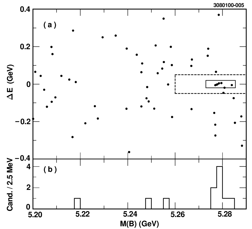
FIG. 1.: (a) The $\Delta E$ vs. $M(B)$ distribution for $B^{0}\to D^{*+}D^{*-}$ candidates for the data taken at the $\Upsilon(4{\rm S})$ resonance. The small rectangle delineates the signal region and the region outside the dashed line is the GSB. (b) The $M(B)$ distribution with the requirement $|\mbox{$\Delta E$}|<20\ {\rm MeV}$.

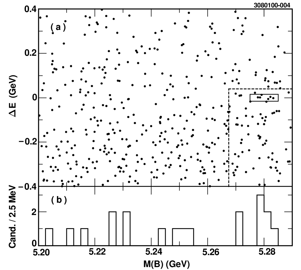
FIG. 2.: (a) The $\Delta E$ vs. $M(B)$ distribution for $B^{0}\to D^{*\pm}D^{\mp}$ candidates for the data taken at the $\Upsilon(4{\rm S})$ resonance. The small rectangle delineates the signal region and the region outside the dashed line is the GSB. (b) The $M(B)$ distribution with the requirement $|\mbox{$\Delta E$}|<16\ {\rm MeV}$.

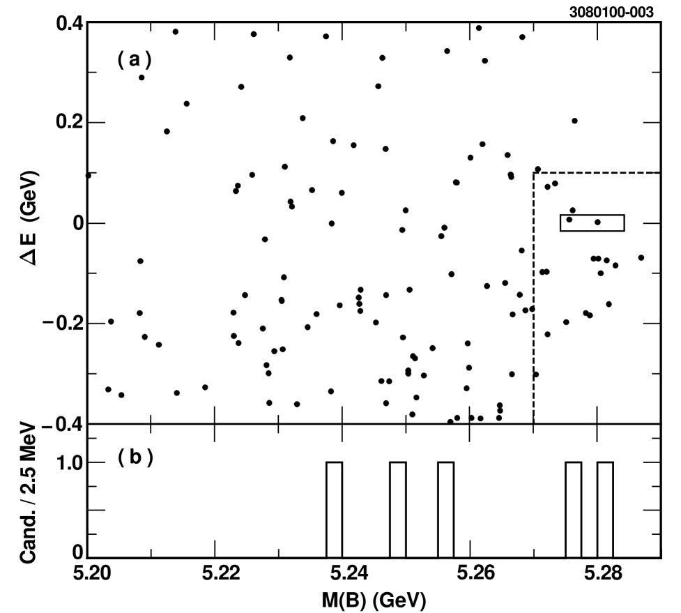
FIG. 3.: (a) The $\Delta E$ vs. $M(B)$ distribution for $B^{0}\to D^{+}D^{-}$ candidates for the data taken at the $\Upsilon(4{\rm S})$ resonance. The small rectangle delineates the signal region and the region outside the dashed line is the GSB. (b) The $M(B)$ distribution with the requirement $|\mbox{$\Delta E$}|<16\ {\rm MeV}$.

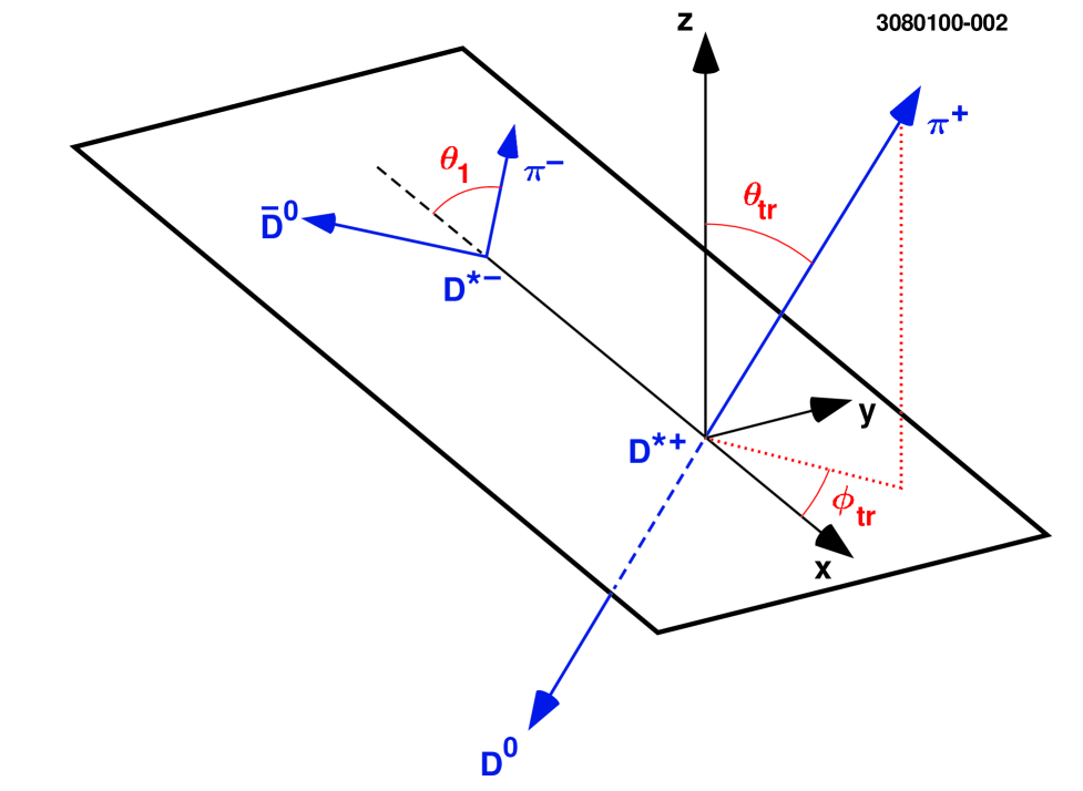
FIG. 4.: The transversity frame for the decay $B^{0}\to D^{*+}D^{*-}$.

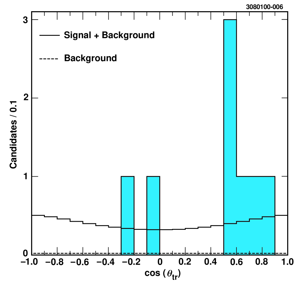
FIG. 5.: The fitted $\cos\mbox{$\theta_{tr}$}$ distribution of the eight $B^{0}\to D^{*+}D^{*-}$ candidates from the signal region. The filled histogram represents the data, the solid line represents the best fit result and the dashed line represents the background component. The fit takes into account the acceptance and resolution in $\cos\mbox{$\theta_{tr}$}$ as described in the text.

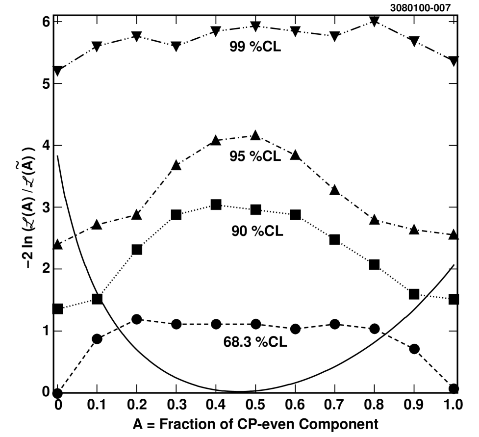
FIG. 6.: $L_{\rm data}(A)\equiv-2\ln({\cal L}(A)/{\cal L}(\tilde{A}))$ for the data (solid curve) compared to $L_{n}$ (Eqn. (5)) for $n=$ 68.3%, 90%, 95% and 99% (broken lines) that correspond to the confidence levels at $n$% for $\alpha=0.34$. See text for details.

REFERENCES

[1]
J.H. Christenson, J.W. Cronin,V.L. Fitch and R. Turlay,
Phys. Rev. Lett. 13, 138 (1964).
[2]
NA31 Collaboration, G.D. Barr et al., Phys. Lett. B 317, 233 (1993);
KTeV Collaboration, A. Alavi-Harati et al., Phys. Rev. Lett 83, 22 (1999);
NA48 Collaboration, V. Fanti et al., Phys. Lett. B 465, 335 (1999).
[3]
OPAL Collaboration, K.Ackerstaff et al., Eur. Phys. J. C 5, 379 (1998);
CDF Collaboration, F. Abe et al., Phys. Rev. Lett. 81, 5513 (1998);
CDF Collaboration, T. Affolder et al., Report no. FERMILAB-PUB-99-225-E,
hep-ex/9909003, submitted to Phys. Rev. D.
[4]
N. Cabibbo, Phys. Rev. Lett. 10, 531 (1963); M. Kobayashi and T. Maskawa, Prog. Theor. Phys. 49, 652 (1973).
[5]
C. Caso et al.,
Particle Data Group, Eur. Phys. J. C3, 1 (1998).
[6]
M. Ciuchini et al.,
Phys. Rev. Lett. 79, 978 (1997).
[7]
A.I. Sanda and Z.-Z. Xing,
Phys. Rev. D 56, 341 (1997).
[8] J.L. Rosner, Phys. Rev. D 42, 3732 (1990).
[9] X.-Y. Pham and Z.-Z. Xing,
Phys. Lett. B 458, 375 (1999).
[10]
I. Dunietz et al.,
Phys. Rev. D 43, 2193 (1991).
[11]
R. Aleksan et al.,
Phys. Lett. B 317, 173 (1993).
[12]The BABAR Physics Book,
P.F. Harrison and H.R. Quinn, Ed., SLAC-R-504.
[13]
Y. Grossman and H.R. Quinn,
Phys. Rev. D 56, 7259 (1997).
[14]
Z.-Z. Xing,
Phys. Lett. B 443, 365 (1998).
[15]
Z.-Z. Xing,
Phys. Rev. D 61, 0140010 (2000).
[16]
R.M. Baxter et al.,
Phys. Rev. D 49, 1594 (1994);
D.S. Hwang and G.-H. Kim,
Phys. Rev. D 53, 3659 (1996);
55, 6944 (1997).
Phys. Rev. D 43, 2193 (1991).
[17]
CLEO Collaboration, M. Artuso et al., Phys. Rev. Lett. 82, 3020 (1999).
[18]
CLEO Collaboration, D.M. Asner et al.,
Phys. Rev. Lett. 79, 799 (1997).
[19]
CLEO Collaboration, Y. Kubota et al.,
Nucl. Instrum. Methods Phys. Res., Sect A 320,
66 (1992).
[20]
T.S. Hill,
Nucl. Instrum. Methods Phys. Res., Sect A 418,
32 (1998).
[21]
In CLEO’s cylindrical coordinate system, the axis coincides
with the direction of the positron beam.
[22] D. Peterson,
Nucl. Phys. B (Proc. Suppl.) 54B, 31 (1997).
[23]
R. Brun et al., GEANT3 Users Guide, CERN DD/EE/84-1.
[24]
CLEO Collaboration, M. Athanas et al.,
Phys. Rev. Lett. 80, 5493 (1998).