We report on measurements of hadronic and leptonic cross sections and leptonic forward-backward asymmetries performed with the L3 detector in the years $1993-95$. A total luminosity of $103\ \mathrm{pb^{-1}}$ was collected at centre-of-mass  energies $\sqrt{s}\approx m_{\mathrm{Z}}$ and $\sqrt{s}\approx m_{\mathrm{Z}}\pm 1.8\ \mathrm{Ge\kern-0.80005ptV}$ which corresponds to 2.5 million hadronic and 245 thousand leptonic events selected. These data lead to a significantly improved determination of $\mathrm{Z}$ parameters. From the total cross sections, combined with our measurements in $1990-92$, we obtain the final results:

$$m_{\mathrm{Z}}=91\,189.8\pm 3.1\ \mathrm{Me\kern-0.80005ptV}\,, \Gamma_{\mathrm{Z}}=2\,502.4\pm 4.2\ \mathrm{Me\kern-0.80005ptV}\,,$$

$$\Gamma_{\mathrm{had}}=1\,751.1\pm 3.8\ \mathrm{Me\kern-0.80005ptV}\,, \Gamma_{\ell}=84.14\pm 0.17\ \mathrm{Me\kern-0.80005ptV}\,.$$

An invisible width of $\Gamma_{\mathrm{inv}}=499.1\pm 2.9\ \mathrm{Me\kern-0.80005ptV}$ is derived which in the Standard Model yields for the number of light neutrino species $N_{\mathrm{\nu}}=2.978\pm 0.014$.

Adding our results on the leptonic forward-backward asymmetries and the tau polarisation, the effective vector and axial-vector coupling constants of the neutral weak current to charged leptons are determined to be $\bar{g}_{\mathrm{V}}^{\mathrm{\ell}}=-0.0397\pm 0.0017$ and $\bar{g}_{\mathrm{A}}^{\mathrm{\ell}}=-0.50153\pm 0.00053$. Including our measurements of the $\mathrm{Z}\rightarrow\mathrm{b\bar{b}}$ forward-backward and quark charge asymmetries a value for the effective electroweak mixing angle of $\sin^{2}\!\overline{\theta}_{\mathrm{W}}=0.23093\pm 0.00066$ is derived.

All these measurements are in good agreement with the Standard Model of electroweak interactions. Using all our measurements of electroweak observables an upper limit on the mass of the Standard Model Higgs boson of $m_{\mathrm{H}}<133\ \mathrm{Ge\kern-0.80005ptV}$ is set at 95% confidence level.

Dedicated to the memory of Prof. Dr. Klaus Schultze

Submitted to The European Physical Journal C

1 Introduction

The Standard Model (SM) of electroweak interactions [1, 2] is tested with great precision by the experiments performed at the LEP and SLC $\mathrm{e^{+}e^{-}}$ colliders running at centre-of-mass energies, $\sqrt{s}$, close to the $\mathrm{Z}$ mass. From measurements of the total cross sections and forward-backward asymmetries in the reactions

$$\mathrm{e^{+}e^{-}}\rightarrow\mathrm{hadrons}(\mathrm{\gamma})\,, \mathrm{e^{+}e^{-}}\rightarrow\mathrm{e^{+}e^{-}}(\mathrm{\gamma})\,,$$

$$\mathrm{e^{+}e^{-}}\rightarrow\mathrm{\mu^{+}\mu^{-}}(\mathrm{\gamma})\,, \mathrm{e^{+}e^{-}}\rightarrow\mathrm{\tau^{+}\tau^{-}}(\mathrm{\gamma})\,,$$ (1)

the mass, total and partial widths of the $\mathrm{Z}$ and other electroweak parameters are obtained by L3 [3, 4] and other experiments [5, 6, 7, 8]. The $(\mathrm{\gamma})$ indicates the presence of radiative photons.

The large luminosity collected in the years $1993-95$ enables a significant improvement on our previous measurements of $\mathrm{Z}$ parameters. An integrated luminosity of $103\ \mathrm{pb^{-1}}$ was collected, corresponding to the selection of $2.5\cdot 10^{6}$ hadronic and $2.5\cdot 10^{5}$ leptonic events. Most of the data were collected at a centre-of-mass energy corresponding to the maximum annihilation cross section.

In 1993 and 1995 scans, of the $\mathrm{Z}$ resonance were performed where runs at the $\mathrm{Z}$ pole alternated with runs at about $1.8\ \mathrm{Ge\kern-1.00006ptV}$ on either side of the peak. Compared to previous measurements, our event samples on the wings of the $\mathrm{Z}$ resonance are increased by more than a factor of five.

The LEP beam energies were precisely calibrated at the three energy points in $1993-95$ using the method of resonant depolarisation [9]. As a result, the contributions to the errors on the $\mathrm{Z}$ mass and total width from the uncertainty on the centre-of-mass energy are reduced by factors of about five and three, respectively, as compared to the data collected before.

The installation of silicon strip detectors in front of the small angle electromagnetic calorimeters allows a much more precise determination of the fiducial volume used for the luminosity measurement [10]. This improvement, together with the reduced theoretical uncertainty on the small angle Bhabha cross section [11, 12], allows more precise measurements of the cross sections, in particular that for $\mathrm{e^{+}e^{-}}\rightarrow\mathrm{hadrons}(\mathrm{\gamma})$. This results in a better determination of the invisible $\mathrm{Z}$ width, from which the number of light neutrino generations is deduced.

In this article measurements of hadronic and leptonic cross sections and leptonic forward-backward asymmetries, obtained from the data collected between 1993 and 1995, are presented. These measurements are combined with our published results from the data collected in $1990-92$ [4]. The complete integrated luminosity collected by L3 at the $\mathrm{Z}$ resonance is $143\ \mathrm{pb^{-1}}$, consisting of about $3.5\cdot 10^{6}$ hadronic and $3.5\cdot 10^{5}$ leptonic events. The results on the properties of the $\mathrm{Z}$ boson and on other electroweak observables presented here are based on the final analyses of the complete data set collected at the $\mathrm{Z}$ resonance.

This article is organised as follows: After a brief description of the L3 detector in Section 2, we summarise in Section 3 features of the $1993-95$ data analysis common to all final states investigated. Section 4 addresses issues related to the LEP centre-of-mass energy. The measurement of luminosity is described in Section 5. The event selection and the analysis of the reactions in (1) are discussed in Sections 6 to 9 and the results on the measurements of total cross sections and forward-backward asymmetries are presented in Section 10. A general description of the fits performed to our data is given in Section 11. Various fits for $\mathrm{Z}$ parameters are performed in Section 12 and the results of the fits in the framework of the SM are given in Section 13. We summarise and conclude in Section 14. The Appendices A and B give details on the treatment of the $t$-channel contributions in $\mathrm{e^{+}e^{-}}\rightarrow\mathrm{e^{+}e^{-}}(\mathrm{\gamma})$ and on technicalities of the fit procedures, respectively.

2 The L3 Detector

The L3 detector [13] consists of a silicon microvertex detector [14], a central tracking chamber, a high resolution electromagnetic calorimeter composed of BGO crystals, a lead-scintillator ring calorimeter at low polar angles [15], a scintillation counter system, a uranium hadron calorimeter with proportional wire chamber readout and an accurate muon spectrometer. Forward-backward muon chambers, completed for the 1995 data taking, extend the polar angle coverage of the muon system down to 24 degrees [16] with respect to the beam line. All detectors are installed in a 12 m diameter magnet which provides a solenoidal field of $0.5\ \mathrm{T}$ in the central region and a toroidal field of $1.2\ \mathrm{T}$ in the forward-backward region. The luminosity is measured using BGO calorimeters preceded by silicon trackers [10] situated on each side of the detector.

In the L3 coordinate system the direction of the $\mathrm{e^{-}}$ beam defines the $z$ direction. The $xy$, or $r\phi$ plane, is the bending plane of the magnetic field, with the $x$ direction pointing to the centre of the LEP ring. The coordinates $\phi$ and $\theta$ denote the azimuthal and polar angles.

3 Data Analysis

The data collected between 1993 and 1995 are split into nine samples according to the year and the centre-of-mass energy. Data samples at $\sqrt{s}\approx m_{\mathrm{Z}}$ are referred to as peak, those at off-peak energies are referred to as peak$-2$ and peak$+2$. The peak samples in 1993 and 1995 are further split into data taken early in the year (pre-scan) and those peak runs interspersed with off-peak data taking (scan) which coincide with the precise LEP energy calibration (see Section 4). Cross sections and leptonic forward-backward asymmetries are determined for each data sample.

Acceptances, background contaminations and trigger efficiencies are studied for all nine data samples separately to take into account their possible dependence on the centre-of-mass energy and the time dependence of the detector status. Systematic errors are determined for the data samples individually. Average values for uncertainties are used if no dependence on the centre-of-mass energy or the data taking period is observed. Correlations of the systematic errors among the data sets are estimated and are taken into account in the analyses to determine electroweak parameters.

Acceptances and background contaminations from $\mathrm{e^{+}e^{-}}$-interactions are determined by Monte Carlo simulations. The following event generator programs are used for the various signal and background processes: JETSET [17] and HERWIG [18] for $\mathrm{e^{+}e^{-}}\rightarrow\mathrm{hadrons}(\mathrm{\gamma})$; KORALZ [19] for $\mathrm{e^{+}e^{-}}\rightarrow\mathrm{\mu^{+}\mu^{-}}(\mathrm{\gamma})$ and $\mathrm{e^{+}e^{-}}\rightarrow\mathrm{\tau^{+}\tau^{-}}(\mathrm{\gamma})$; BHAGENE [20], BHWIDE [21] and BABAMC [22] for large angle $\mathrm{e^{+}e^{-}}\rightarrow\mathrm{e^{+}e^{-}}(\mathrm{\gamma})$; BHLUMI [11] for small angle $\mathrm{e^{+}e^{-}}\rightarrow\mathrm{e^{+}e^{-}}(\mathrm{\gamma})$; GGG [23] for $\mathrm{e^{+}e^{-}}\rightarrow\mathrm{\gamma}\mathrm{\gamma}(\mathrm{\gamma})$; DIAG36 [24] for $\mathrm{e^{+}e^{-}}\rightarrow\mathrm{e^{+}e^{-}}\,\mathrm{\ell^{+}\ell^{-}}$; DIAG36, PHOJET [25] and PYTHIA [17] for $\mathrm{e^{+}e^{-}}\rightarrow\mathrm{e^{+}e^{-}}\,\mathrm{hadrons}$. For the simulation of hadronic final states the fragmentation parameters of JETSET and HERWIG are tuned to describe our data as discussed in Reference [26].

The generated events are passed through a complete detector simulation. The response of the L3 detector is modelled with the GEANT [27] detector simulation program which includes the effects of energy loss, multiple scattering and showering in the detector materials. Hadronic showers are simulated with the GHEISHA [28] program. The performance of the detector, including inefficiencies and their time dependence as observed during data taking, is taken into account in the simulation. With this procedure, experimental systematic errors on cross sections and forward-backward asymmetries are minimized.

4 LEP Energy Calibration

The average centre-of-mass energy of the colliding particles at the L3 interaction point is calculated using the results provided by the Working Group on LEP Energy [9]. Every 15 minutes the average centre-of-mass energy is determined from measured LEP machine parameters, applying the energy model which is based on calibration by resonant depolarisation [29]. This model traces the time variation of the centre-of-mass energy of typically $1\ \mathrm{Me\kern-1.00006ptV}$ per hour. The average centre-of-mass energies are calculated for each data sample individually as luminosity weighted averages. Slightly different values are obtained for different reactions because of small differences in the usable luminosity.

The errors on the centre-of-mass energies and their correlations for the 1994 data and for the two scans performed in 1993 and 1995 are given in form of a $7\times 7$ covariance matrix in Table 1. The uncertainties on the centre-of-mass energy for the data samples not included in this matrix, i.e. the 1993 and 1995 pre-scans, are $18\ \mathrm{Me\kern-1.00006ptV}$ and $10\ \mathrm{Me\kern-1.00006ptV}$, respectively. Details of the treatment of these errors in the fits can be found in Appendix B.

The energy distribution of the particles circulating in an $\mathrm{e^{+}e^{-}}$-storage ring has a finite width due to synchrotron oscillations. An experimentally observed cross section is therefore a convolution of cross sections at energies which are distributed around the average value in a gaussian form. The spread of the centre-of-mass energy for the L3 interaction point as obtained from the observed longitudinal length of the particle bunches in LEP is listed in Table 2 [9]. The time variation of the average energy causes a similar, but smaller, effect which is included in these numbers.

All cross sections and forward-backward asymmetries quoted below are corrected for the energy spread to the average value of the centre-of-mass energy. The relative corrections on the measured hadronic cross sections amount to $+1.7$ per mill () at the $\mathrm{Z}$ pole and to $-1.1$ and $-0.6$ at the peak$-2$ and peak$+2$ energy, respectively. The absolute corrections on the forward-backward asymmetries are very small. The largest correction is $-0.0002$ for the muon and tau peak$-2$ data sets. The error on the energy spread is propagated into the fits, resulting in very small contributions to the errors of the fitted parameters (see Appendix B). The largest effect is on the total width of the $\mathrm{Z}$, contributing approximately $0.3\ \mathrm{Me\kern-1.00006ptV}$ to its error.

During the operation of LEP, no evidence for an average longitudinal polarisation of the electrons or positrons has been observed. Stringent limits on residual polarisation during luminosity runs are set such that the uncertainties on the determination of electroweak observables are negligible compared to their experimental errors [30].

The determination of the LEP centre-of-mass energy in $1990-92$ is described in References [31]. From these results the LEP energy error matrix given in Table 3 is derived.

5 Luminosity Measurement

The integrated luminosity ${\cal L}$ is determined by measuring the number of small-angle Bhabha interactions $\mathrm{e^{+}e^{-}}\rightarrow\mathrm{e^{+}e^{-}}(\mathrm{\gamma})$. For this purpose two cylindrical calorimeters consisting of arrays of BGO crystals are located on either side of the interaction point. Both detectors are divided into two half-rings in the vertical plane to allow the opening of the detectors during filling of LEP. A silicon strip detector, consisting of two layers measuring the polar angle, $\theta$, and one layer measuring the azimuthal angle, $\phi$, is situated in front of each calorimeter to precisely define the fiducial volume. A detailed description of the luminosity monitor and the luminosity determination can be found in Reference [10].

The selection of small-angle Bhabha events is based on the energy depositions in adjacent crystals of the BGO calorimeters which are grouped to form clusters. The highest-energy cluster on each side is considered for the luminosity analysis. For about 98% of the cases a hit in the silicon detectors is matched with a cluster and its coordinate is used; otherwise the BGO coordinate is retained.

The event selection criteria are:

1. The energy of the most energetic cluster is required to exceed $0.8E_{\mathrm{b}}$ and the energy on the opposite side must be greater than $0.4E_{\mathrm{b}}$, where $E_{\mathrm{b}}$ is the beam energy. If the energy of the most energetic cluster is within $\pm 5\%$ of $E_{\mathrm{b}}$ the minimum energy requirement on the opposite side is reduced to $0.2E_{\mathrm{b}}$ in order to recover events with energy lost in the gaps between crystals. The distributions of the energy of the most energetic cluster and the cluster on the opposite side as measured in the luminosity monitors are shown in Figure 1 for the 1993 data. All selection cuts except the one under study are applied.

2. The cluster on one side must be confined to a tight fiducial volume:

   • 32 mrad $<\theta<$ 54 mrad; $|\phi-90^{\circ}|>11.25^{\circ}$ and $|\phi-270^{\circ}|>11.25^{\circ}$.

   The requirements on the azimuthal angle remove the regions where the half-rings of the detector meet. The cluster on the opposite side is required to be within a larger fiducial volume:

   • 27 mrad $<\pi-\theta<$ 65 mrad; $|\phi-90^{\circ}|>3.75^{\circ}$ and $|\phi-270^{\circ}|>3.75^{\circ}$.

   This ensures that the event is fully contained in the detectors and edge effects in the reconstruction are avoided.

3. The coplanarity angle $\Delta\phi=\phi(z<0)-\phi(z>0)$ between the two clusters must satisfy $|\Delta\phi-180^{\circ}|<10^{\circ}$.

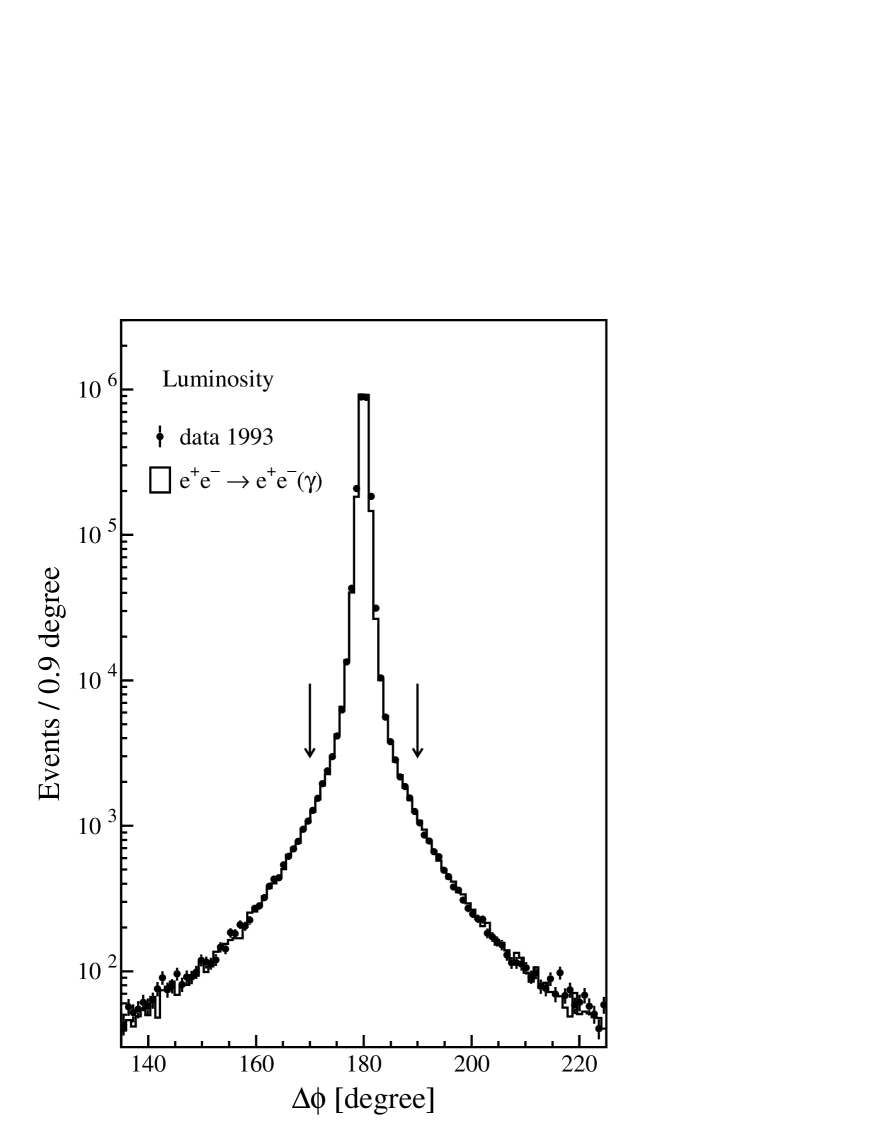
Figure 2: The distribution of the coplanarity angle $\Delta\phi$ for small angle Bhabha candidates.

The distribution of the coplanarity angle is shown in Figure 2. Very good agreement with the Monte Carlo simulation is observed.

Four samples of Bhabha events are defined by applying the tight fiducial volume cut to one of the $\theta$-measuring silicon layers. Taking the average of the luminosities obtained from these samples minimizes the effects of relative offsets between the interaction point and the detectors. The energy and coplanarity cuts reduce the background from random beam-gas coincidences. The remaining contamination is very small: $(3.4\pm 2.2)\cdot 10^{-5}$. This number is estimated using the sidebands of the coplanarity distribution, $10^{\circ}<|\Delta\phi-180^{\circ}|<30^{\circ}$, after requiring that neither of the two clusters have an energy within $\pm 5\%$ of $E_{\mathrm{b}}$.

The accepted cross section is determined from Monte Carlo $\mathrm{e^{+}e^{-}}\rightarrow\mathrm{e^{+}e^{-}}(\mathrm{\gamma})$ samples generated with the BHLUMI event generator at a fixed centre-of-mass energy of $\sqrt{s}=91.25\ \mathrm{Ge\kern-1.00006ptV}$. The dependence on the centre-of-mass energy, as well as the contributions of $\mathrm{Z}$-exchange and $\mathrm{\gamma}\mathrm{Z}$ interference, are calculated with the BHLUMI program. At $\sqrt{s}=91.25\ \mathrm{Ge\kern-1.00006ptV}$ the accepted cross section is determined to be $69.62\ \mathrm{nb}$. The statistical error on the Monte Carlo sample contributes $0.35$ to the uncertainty of the luminosity measurement. The theoretical uncertainty on the Bhabha cross section in our fiducial volume is estimated to be $0.61$ [12].

The experimental errors of the luminosity measurement are small. Important sources of systematic errors are: geometrical uncertainties due to the internal alignment of the silicon detectors ($0.15$ to $0.27$), temperature expansion effects ($0.14$) and the knowledge on the longitudinal position of the silicon detectors ($0.16$ to $0.60$). The precision depends on the accuracy of the detector surveys and on the stability of the detector and wafer positions during the different years.

The polar angle distribution of Bhabha scattering events used for the luminosity measurement is shown in Figure 3. The structure seen in the central part of the $+z$ side is due to the flare in the beam pipe on this side. The imperfect description in the Monte Carlo does not pose any problem as it is far away from the edges of the fiducial volume.

The overall agreement between the data and Monte Carlo distributions of the selection quantities is good. Small discrepancies in the energy distributions at high energies are due to contamination of Bhabha events with beam-gas interactions and, at low energies, due to an imperfect description of the cracks between crystals. The selection uncertainty is estimated by varying the selection criteria over reasonable ranges and summing in quadrature the resulting contributions. This procedure yields errors between $0.42$ and $0.48$ for different years. The luminosities determined from the four samples described above agree within these errors. The trigger inefficiency is measured using a sample of events triggered by only requiring an energy deposit exceeding $30\ \mathrm{Ge\kern-1.00006ptV}$ on one side. It is found to be negligible.

The various sources of uncertainties are summarized in Table 4. Combining them in quadrature yields total experimental errors on the luminosity of $0.86$, $0.64$ and $0.68$ in 1993, 1994 and 1995. Correlations of the total experimental systematic errors between different years are studied and the correlation matrix is given in Table 5. The error from the theory is fully correlated.

Because of the $1/s$ dependence of the small angle Bhabha cross section, the uncertainty on the centre-of-mass energies causes a small additional uncertainty on the luminosity measurement. For instance, this amounts to $0.1$ for the high statistics data sample of 1994. This effect is included in the fits performed in Section 12 and 13, see Appendix B.

The statistical error on the luminosity measurement from the number of observed small angle Bhabha events is also included in those fits. Table 6 lists the number of observed Bhabha events for the nine data samples and the corresponding errors on cross section measurements. Combining all data sets taken in $1993-95$ at $\sqrt{s}\approx m_{\mathrm{Z}}$ the statistical error on the luminosity contributes 0.45 to the uncertainty on the pole cross section measurements.

Higher order corrections from photon radiation to the small angle Bhabha cross section are studied with the photon spectrum of luminosity events. For this analysis events with two distinct energy clusters exceeding $0.1E_{\mathrm{b}}$ in one of the calorimeters are selected. The photon is identified as the lower energy cluster. The fraction of radiative events with $E_{\gamma}>0.1E_{\mathrm{b}}$ in the total low-angle Bhabha sample is 2% and the measured cross section, normalised to the expectation, is found to be $0.993\pm 0.16$. The observed spectrum from 1993 is shown in Figure 4 and good agreement is found with the Monte Carlo expectation.

6 $\mathrm{e^{+}e^{-}}\rightarrow\mathrm{hadrons}(\mathrm{\gamma})$

Event Selection

Hadronic $\mathrm{Z}$ decays are identified by their large energy deposition and high multiplicity in the electromagnetic and hadron calorimeters. The selection criteria are similar to those applied in our previous analysis [4]:

1. The total energy observed in the detector, $E_{\mathrm{vis}}$, normalised to the centre-of-mass energy must satisfy $0.5<E_{\mathrm{vis}}/\sqrt{s}<2.0$;

2. The energy imbalance along the beam direction, $E_{\parallel}$, must satisfy $|E_{\parallel}|/E_{\mathrm{vis}}<0.6$;

3. The transverse energy imbalance, $E_{\perp}$, must satisfy $E_{\perp}/E_{\mathrm{vis}}<0.6$;

4. The number of clusters, $N_{\mathrm{cl}}$, formed from energy depositions in the calorimeters is required to be:
   a) $N_{\mathrm{cl}}\geq 13$ for $|\cos\theta_{t}|\leq 0.74$ (barrel region),
   b) $N_{\mathrm{cl}}\geq 17$ for $|\cos\theta_{t}|>0.74$ (end-cap region),
   where $\theta_{t}$ is the polar angle of the event thrust axis.

Detailed analyses of the large data samples collected have been used to improve the Monte Carlo simulation of the detector response. Figures 5 to 9 show the distributions of the quantities used to select hadronic $\mathrm{Z}$ decays and the comparisons to the Monte Carlo predictions. In these plots all selection cuts are applied, except the one under study. Good agreement is observed between our data and the Monte Carlo simulations.

Total Cross Section

The acceptance for $\mathrm{e^{+}e^{-}}\rightarrow\mathrm{hadrons}(\mathrm{\gamma})$ events is determined from large samples of Monte Carlo events generated with the JETSET program. Applying the selection cuts, between $99.30\%$ and $99.42\%$ of the events are accepted depending on the year of the data taking and on differences in initial-state photon radiation at the various centre-of-mass energies. Monte Carlo events are generated with $\sqrt{s^{\prime}}>0.1\sqrt{s}$ where $\sqrt{s^{\prime}}$ is the effective centre-of-mass energy after initial state photon radiation. The acceptance for events in the data with $\sqrt{s^{\prime}}\leq 0.1\sqrt{s}$ is estimated to be negligible. They are not considered as part of the signal and hence not corrected for.

The interference between initial and final state photon radiation is not accounted for in the event generator. This effect modifies the angular distribution of the events in particular at very low polar angles where the detector inefficiencies are largest. However, the error from the imperfect simulation on the measured cross section, which includes initial-final state interference as part of the signal, is estimated to be very small ($\ll 0.1\ \mathrm{pb}$) in the centre-of-mass energy range considered here. Quark pairs originating from pair production from initial state radiation are considered as part of the signal if their invariant mass exceeds 50% of $\sqrt{s}$.

To estimate the uncertainty on the acceptance on the modelling of the quark fragmentation, the determination of the acceptance is repeated using the HERWIG program. The detector simulations of both Monte Carlo programs are tuned in the same way to describe as closely as possible our data, e.g. in terms of energy resolution and cluster multiplicity. The remaining difference in acceptance is $0.42$ and we assign half of it as an estimate of the uncertainty on the acceptance of $\mathrm{e^{+}e^{-}}\rightarrow\mathrm{hadrons}(\mathrm{\gamma})$ events due to the modelling of quark fragmentation. Differences of the implementation of QED effects in both programs are studied and found to have negligible impact on the acceptance.

Hadronic $\mathrm{Z}$ decays are triggered by the energy, central track, muon or scintillation counter multiplicity triggers. The combined trigger efficiency is obtained from the fraction of events with one of these triggers missing as a function of the polar angle of the event thrust axis. This takes into account most of the correlations among triggers. A sizeable inefficiency is only observed for events in the very forward region of the detector, where hadrons can escape through the beam pipe. Trigger efficiencies, including all steps of the trigger system, between $99.829\%$ and $99.918\%$ are obtained for the various data sets. Trigger inefficiencies determined for data sets taken in the same year are statistically compatible. Combining those data sets results in statistical errors of at most $0.12$ which is assigned as systematic error to all data sets.

The background from other $\mathrm{Z}$ decays is found to be small: $2.9$ essentially only from $\mathrm{e^{+}e^{-}}\rightarrow\mathrm{\tau^{+}\tau^{-}}(\mathrm{\gamma})$. The uncertainty on this number is negligible compared to the total systematic error.

The determination of the non-resonant background, mainly $\mathrm{e^{+}e^{-}}\rightarrow\mathrm{e^{+}e^{-}}\,\mathrm{hadrons}$, is based on the measured distribution of the visible energy shown in Figure 5. The Monte Carlo program PHOJET is used to simulate two-photon collision processes. The absolute cross section is derived by scaling the Monte Carlo to obtain the best agreement with our data in the low end of the $E_{\mathrm{vis}}$ spectrum: $0.32\leq E_{\mathrm{vis}}/\sqrt{s}\leq 0.44$. Consistently for all data sets, scale factors of $1.1$ are necessary. In the signal region contaminations from $\mathrm{e^{+}e^{-}}\rightarrow\mathrm{e^{+}e^{-}}\,\mathrm{hadrons}$ between $11.6\ \mathrm{pb}$ and $13.0\ \mathrm{pb}$ are obtained for the different data sets. No dependence on $\sqrt{s}$ is observed. This is in agreement with results of a similar calculation performed with the DIAG36 program.

Beam related background (beam-gas and beam-wall interactions) is small. To the extent that the $E_{\mathrm{vis}}$ spectrum is similar to that of $\mathrm{e^{+}e^{-}}\rightarrow\mathrm{e^{+}e^{-}}\,\mathrm{hadrons}$, it is accounted for by determining the absolute normalisation from the data.

As a check, the non-resonant background is estimated by extrapolating an exponential dependence of the $E_{\mathrm{vis}}$ spectrum from the low energy part into the signal region. This method yields consistent results. Based on these studies we assign an error on the measured hadron cross section of $3\ \mathrm{pb}$ due to the understanding of the non-resonant background. This error assignment is supported by our measurements of the hadronic cross section at high energies ($130\ \mathrm{Ge\kern-1.00006ptV}\leq\sqrt{s}\leq 172\ \mathrm{Ge\kern-1.00006ptV}$) where the relative contribution of two-photon processes is much larger [32, 33]. The extrapolation of these studies back to the $\mathrm{Z}$ peak yields a similar result for the uncertainty.

The contribution of random uranium noise and electronic noise in the detector faking a signal event is determined from a subsample of the event candidates. This subsample is obtained requiring that most of the observed energy stems either from the electromagnetic or the hadron calorimeter and that there be little matching between individual energy deposits and tracks. The $E_{\perp}/E_{\mathrm{vis}}$ distribution of this subsample shows an $\mathrm{e^{+}e^{-}}\rightarrow\mathrm{hadrons}(\mathrm{\gamma})$ signal over a flat background (see Figure 10 for the 1994 data). This background is consistent with a constant noise rate, from which a background correction of $7.4\ \mathrm{pb}$ is derived. An uncertainty of $1\ \mathrm{pb}$ on the hadron cross section is assigned to all data sets from this correction. The absolute normalisation of the $\mathrm{e^{+}e^{-}}\rightarrow\mathrm{hadrons}(\mathrm{\gamma})$ signal in Figure 10 is not expected to be perfectly reproduced by the Monte Carlo simulation. However, this does not pose a serious problem as the noise rate is determined from the tail of the spectrum.

The systematic error from event selection on the measured cross sections is estimated by varying the selection cuts. All cross section results are stable within $\pm 0.3$. The systematic errors to the cross section measurements $\mathrm{e^{+}e^{-}}\rightarrow\mathrm{hadrons}(\mathrm{\gamma})$ are summarised in Table 7. Uncertainties which scale with the cross section and absolute uncertainties are separated because they translate in a different way into errors on $\mathrm{Z}$ parameters, in particular on the total width. The scale error is further split into a part uncorrelated among the data samples, in this case consisting of the contribution of Monte Carlo statistics, and the rest which is taken to be fully correlated and amounts to $0.39$.

The results of the $\mathrm{e^{+}e^{-}}\rightarrow\mathrm{hadrons}(\mathrm{\gamma})$ cross section measurements are discussed in Section 10.

7 $\mathrm{e^{+}e^{-}}\rightarrow\mathrm{\mu^{+}\mu^{-}}(\mathrm{\gamma})$

Event Selection

The selection of $\mathrm{e^{+}e^{-}}\rightarrow\mathrm{\mu^{+}\mu^{-}}(\mathrm{\gamma})$ in the 1993 and 1994 data is similar to the selection applied in previous years described in Reference [4]. Two muons in the polar angular region $|\cos\theta|<0.8$ are required. Most of the muons, 88%, are identified by a reconstructed track in the muon spectrometer. Muons are also identified by their minimum ionising particle (MIP) signature in the inner sub-detectors, if less than two muon chamber layers are hit. A muon candidate is denoted as a MIP, if at least one of the following conditions is fulfilled:

1. A track in the central tracking chamber must point within $5^{\circ}$ in azimuth to a cluster in the electromagnetic calorimeter with an energy less than 2 $\mathrm{Ge\kern-1.00006ptV}$.

2. On a road from the vertex through the barrel hadron calorimeter, at least five out of a maximum of 32 cells must be hit, with an average energy of less than 0.4 $\mathrm{Ge\kern-1.00006ptV}$ per cell.

3. A track in the central chamber or a low energy electromagnetic cluster must point within $10^{\circ}$ in azimuth to a muon chamber hit.

In addition, both the electromagnetic and the hadronic energy in a cone of $12^{\circ}$ half-opening angle around the MIP candidate, corrected for the energy loss of the particle, must be less than 5 $\mathrm{Ge\kern-1.00006ptV}$.

Events of the reaction $\mathrm{e^{+}e^{-}}\rightarrow\mathrm{\mu^{+}\mu^{-}}(\mathrm{\gamma})$ are selected by the following criteria:

1. The event must have a low multiplicity in the calorimeters $N_{\mathrm{cl}}\leq 15$.

2. If at least one muon is reconstructed in the muon chambers, the maximum muon momentum must satisfy $p_{\mathrm{max}}>0.6\,E_{\mathrm{b}}$. If both muons are identified by their MIP signature there must be two tracks in the central tracking chamber with at least one with a transverse momentum larger than $3\ \mathrm{Ge\kern-1.00006ptV}$.

3. The acollinearity angle $\xi$ must be less than $90^{\circ}$, $40^{\circ}$ or $5^{\circ}$ if two, one or no muons are reconstructed in the muon chambers.

4. The event must be consistent with an origin of an $\mathrm{e^{+}e^{-}}$-interaction requiring at least one time measurement of a scintillation counter, associated to a muon candidate, to coincide within $\pm 3\ \mathrm{ns}$ with the beam crossing. Also, there must be a track in the central tracking chamber  with a distance of closest approach to the beam axis of less than $5\ \mathrm{mm}$.

As an example, Figure 11 shows the distribution of the maximum measured muon momentum for candidates in the $1993-94$ data compared to the expectation for signal and background processes. The acollinearity angle distribution of the selected muon pairs is shown in Figure 12. The experimental angular resolution and radiation effects are well reproduced by the Monte Carlo simulation.

The analysis of the 1995 data in addition uses the newly installed forward-backward muon chambers. The fiducial volume is extended to $|\cos\theta|<$ 0.9. Each event must have at least one track in the central tracking chamber with a distance of closest approach in the transverse plane of less than $1\ \mathrm{mm}$ and a scintillation counter time coinciding within $\pm 5\ \mathrm{ns}$ with the beam crossing. The rejection of cosmic ray muons in the 1995 data is illustrated in Figure 13.

For events with muons reconstructed in the muon chambers the maximum muon momentum must be larger than $\frac{2}{3}\,E_{\mathrm{b}}$. Every muon without a reconstructed track in the muon chambers must have a transverse momentum larger than $3\ \mathrm{Ge\kern-1.00006ptV}$ as measured in the central tracking chamber. The polar angle distribution of muon pairs collected in 1995 is shown in Figure 14.

Total Cross Section

The acceptance for the process $\mathrm{e^{+}e^{-}}\rightarrow\mathrm{\mu^{+}\mu^{-}}(\mathrm{\gamma})$ in the fiducial volume $|\cos\theta|<0.8$ (0.9 for 1995 data) and for $\xi<90^{\circ}$ is determined with events generated with the KORALZ program. We obtain acceptances between $92.25\%$ and $93.04\%$, mainly depending on the centre-of-mass energy. The systematic error on the cross section from imperfect description of detector inefficiencies is estimated to be $2.7$ (3.2 for the 1995 data). This number is calculated from a comparison with results obtained by removing events at the detector edges from the analysis and using different descriptions of time dependent detector inefficiencies. Smaller contributions to the systematic error arise from the statistical precision of the Monte Carlo simulations performed for the different data samples.

Muon pairs are mainly triggered by the muon and the central track trigger. The trigger efficiencies are studied as a function of the azimuthal angle as inefficiencies are expected close to chamber boundaries. For the 1995 data also the polar angular dependence of the trigger efficiency is determined to account for effects in the forward region. Events with both muons reconstructed in the muon chambers are triggered with full efficiency. The efficiency of the central track trigger is independently determined using Bhabha events. The overall trigger efficiency varies between $99.62\%$ and $99.90\%$ for the different years of data taking. Systematic errors on the measured cross sections of less than $1$ are estimated from comparing a simulation of the central track trigger efficiency and its measurement with Bhabha events.

A background of $(1.35\pm 0.03)\%$ remains in the sample arising from $\mathrm{e^{+}e^{-}}\rightarrow\mathrm{\tau^{+}\tau^{-}}(\mathrm{\gamma})$ events with both tau leptons decaying into muons. The error reflects Monte Carlo statistics and the uncertainty of the branching ratio $\mathrm{\tau^{-}\rightarrow\mu^{-}\bar{\nu}_{\mu}\nu_{\tau}}$ [34]. Other backgrounds from $\mathrm{Z}$ decays are smaller than $0.1$. The contamination from the non-resonant two-photon process $\mathrm{e^{+}e^{-}}\rightarrow\mathrm{e^{+}e^{-}}\,\mathrm{\mu^{+}\mu^{-}}$ is $0.11\ \mathrm{pb}$, i.e. between $0.1$ and $0.3$ of the signal cross section, as determined using the DIAG36 Monte Carlo program.

The residual contamination from cosmic ray muons in the event sample is determined from the sideband in the distribution of distance of closest approach to the beam axis after all other selection cuts are applied (Figure 13). Cosmic ray muons enter into the event sample at a rate of $(9.7\pm 0.8)\cdot 10^{-4}$ per minute of data taking which translates to background contaminations between $1.9$ and $6.8$ for the different data sets depending on their average instantaneous luminosity and the signal cross section. The statistical precision of the determination of the cosmic contamination causes a systematic error of $0.3\ \mathrm{pb}$ on the total muon pair cross section.

By varying the selection cuts we determine systematic errors on the total cross section between $1.3$ and $2.2$. The systematic errors on the cross section measurements $\mathrm{e^{+}e^{-}}\rightarrow\mathrm{\mu^{+}\mu^{-}}(\mathrm{\gamma})$ are summarised in Table 8.

Resonant four-fermion final states with a high-mass muon pair and a low-mass fermion pair are accepted. These events are considered as part of the signal if the invariant mass of the muon pair exceeds $0.5\sqrt{s}$. This inclusive selection minimizes errors due to higher order radiative corrections. Especially no cut is applied on additional tracks from low-mass fermion pairs in the final state [35].

Forward-Backward Asymmetry

The forward-backward asymmetry, $A_{\mathrm{FB}}$, is defined as:

$$A_{\mathrm{FB}}=\frac{\sigma_{\mathrm{F}}-\sigma_{\mathrm{B}}}{\sigma_{\mathrm{F}}+\sigma_{\mathrm{B}}}\,,$$ (2)

where $\sigma_{\mathrm{F}}$ is the cross section for events with the fermion scattered into the hemisphere which is forward with respect to the $\mathrm{e^{-}}$ beam direction. The cross section in the backward hemisphere is denoted by $\sigma_{\mathrm{B}}$. Events with hard photon bremsstrahlung are removed from the sample by requiring that the acollinearity angle of the event be less than $15^{\circ}$. The differential cross section in the angular region $|\cos\theta|<0.9$ can then be approximated by the lowest order angular dependence to sufficient precision:

$$\frac{\mathrm{d}\sigma}{\mathrm{d}\!\cos\theta}\propto\frac{3}{8}\left(1+\cos^{2}\theta\right)+A_{\mathrm{FB}}\cos\theta\,,$$ (3)

with $\theta$ being the polar angle of the final state fermion with respect to the $\mathrm{e^{-}}$ beam direction.

For each data set the forward-backward asymmetry is determined from a maximum likelihood fit to our data where the likelihood function is defined as the product over the selected events labelled $i$ of the differential cross section evaluated at their respective scattering angle $\theta_{i}$:

$$L=\prod_{i}\left(\frac{3}{8}\left(1+\cos^{2}\theta_{i}\right)+\left(1-2\kappa_{i}\right)A_{\mathrm{FB}}\cos\theta_{i}\right).$$ (4)

The probability of charge confusion for a specific event, $\kappa_{i}$, is included in the fit. Only events with opposite charge assignment to the two muons are used for this measurement. The bias on the asymmetry measurement introduced by the use of the lowest order angular dependence (Equation 3) does not exceed 0.0003.

This method does not require an exact knowledge of the acceptance as a function of the polar angle provided that the acceptance is independent of the muon charge. Events without a reconstructed muon in the muon chambers are included with the charge assignment obtained from the central tracking chamber in a similar way as for $\mathrm{e^{+}e^{-}}$ final states [4]. This largely reduces effects of charge dependent acceptance in the muon chambers. The remaining asymmetry is estimated by artificially symmetrising the detector. For each known, inefficient detector element, the element opposite with respect to the centre of the detector is removed from the data reconstruction. The event selection is applied again and, for the large 1994 data set, the measured forward-backward asymmetry changes by $0.0011\pm 0.0006$. Half of this difference, $0.0006$, is assigned to all data sets as a systematic error on $A_{\mathrm{FB}}$ from a possible detector asymmetry. In 1995 the forward-backward muon chambers did not contribute significantly to the detector asymmetry.

The values of $\kappa_{i}$ are obtained from the fraction of events with identical charges assigned to both muons. Besides its dependence on the transverse momentum, the charge measurement strongly depends on the number of muon chamber layers used in the reconstruction. The charge confusion is determined for each event class individually. The average charge confusion probability, almost entirely caused by muons only measured in the central tracking chamber, is $(3.2\pm 0.3)$, $(0.8\pm 0.1)$ and $(1.0\pm 0.3)$ for the years 1993, 1994 and 1995, respectively, where the errors are statistical. The improvement in the charge determination for 1994 and 1995 reflects the use of the silicon microvertex detector.

The correction for charge confusion is proportional to the forward-backward asymmetry and it is less than $0.001$ for all data sets. To estimate a possible bias from a preferred orientation of events with the two muons measured to have the same charge we determine the forward-backward asymmetry of these events using the track with a measured momentum closer to the beam energy. The asymmetry of this subsample is statistically consistent with the standard measurement. Including these like-sign events in the 1994 sample would change the measured asymmetry by $0.0008$. Half of this number is taken as an estimate of a possible bias of the asymmetry measurement from charge confusion in the $1993-94$ data. The same procedure is applied to the 1995 data and the statistical precision limits a possible bias to $0.0010$.

Differences of the momentum reconstruction in forward and backward events would cause a bias of the asymmetry measurement because of the requirement on the maximum measured muon momentum. We determine the loss of efficiency due to this cut separately for forward and backward events by selecting muon pairs without cuts on the reconstructed momentum. No significant difference is observed and the statistical error of this comparison limits the possible effect on the forward-backward asymmetry to be less than $0.0004$ and $0.0009$ for the $1993-94$ and 1995 data, respectively.

Other possible biases from the selection cuts on the measurement of the forward-backward asymmetry are negligible. This is verified by a Monte Carlo study which shows that events not selected for the asymmetry measurement, but inside the fiducial volume and with $\xi<15^{\circ}$, do not have a different $A_{\mathrm{FB}}$ value.

The background from $\mathrm{e^{+}e^{-}}\rightarrow\mathrm{\tau^{+}\tau^{-}}(\mathrm{\gamma})$ events is found to have the same asymmetry as the signal and thus neither necessitates a correction nor causes a systematic uncertainty. The effect of the contribution from the two-photon process $\mathrm{\mathrm{e^{+}e^{-}}\rightarrow\mathrm{e^{+}e^{-}}\,\mathrm{\mu^{+}\mu^{-}}}$, further reduced by the tighter acollinearity cut on the measured muon pair asymmetry, can be neglected. The forward-backward asymmetry of the cosmic ray muon background is measured to be $-0.02\pm 0.13$ using the events in the sideband of the distribution of closest approach to the interaction point. Weighted by the relative contribution to the data set this leads to corrections of $-0.0007$ and $+0.0003$ to the peak$-2$ and peak$+2$ asymmetries, respectively. On the peak this correction is negligible. The statistical uncertainty of the measurement of the cosmic ray asymmetry causes a systematic error of $0.0001$ on the peak and between $0.0003$ and $0.0005$ for the peak$-2$ and peak$+2$ data sets.

The systematic uncertainties on the measurement of the muon forward-backward asymmetry are summarised in Table 9. In $1993-94$ the total systematic error amounts to $0.0008$ at the peak points and to $0.0009$ at the off-peak points due to the larger contamination of cosmic ray muons. For the 1995 data the determination of systematic errors is limited by the number of events taken with the new detector configuration and the total error is estimated to be $0.0015$.

In Figure 15 the differential cross sections $\mathrm{d}\sigma/\mathrm{d}\!\cos\theta$ measured from the $1993-95$ data sets are shown for three different centre-of-mass energies. The data are corrected for detector acceptance and charge confusion. Data sets with a centre-of-mass energy close to $m_{\mathrm{Z}}$, as well as the data at peak$-2$ and the data at peak$+2$, are combined. The data are compared to the differential cross section shape given in Equation 3.

The results of the total cross section and forward-backward asymmetry measurements in $\mathrm{e^{+}e^{-}}\rightarrow\mathrm{\mu^{+}\mu^{-}}(\mathrm{\gamma})$ are presented in Section 10.

8 $\mathrm{e^{+}e^{-}}\rightarrow\mathrm{\tau^{+}\tau^{-}}(\mathrm{\gamma})$

Event Selection

The selection of $\mathrm{e^{+}e^{-}}\rightarrow\mathrm{\tau^{+}\tau^{-}}(\mathrm{\gamma})$ events aims to select all hadronic and leptonic decay modes of the tau. $\mathrm{Z}$ decays into tau leptons are distinguished from other $\mathrm{Z}$ decays by the lower visible energy due to the presence of neutrinos and the lower particle multiplicity as compared to hadronic $\mathrm{Z}$ decays. Compared to our previous analysis [4] the selection of $\mathrm{e^{+}e^{-}}\rightarrow\mathrm{\tau^{+}\tau^{-}}(\mathrm{\gamma})$ events is extended to a larger polar angular range, $|\cos\theta_{t}|\leq 0.92$, where $\theta_{t}$ is defined by the thrust axis of the event.

Event candidates are required to have a jet, constructed from calorimetric energy deposits [36] and muon tracks, with an energy of at least $8\ \mathrm{Ge\kern-1.00006ptV}$. Energy deposits in the hemisphere opposite to the direction of this most energetic jet are combined to form a second jet. The two jets must have an acollinearity angle $\xi<10^{\circ}$. There is no energy requirement on the second jet.

High multiplicity hadronic $\mathrm{Z}$ decays are rejected by allowing at most three tracks matched to any of the two jets. In each of the two event hemispheres there should be no track with an angle larger than $18^{\circ}$ with respect to the jet axis. Resonant four-fermion final states with a high mass tau pair and a low mass fermion pair are mostly kept in the sample. The multiplicity cut affects only tau decays into three charged particles with the soft fermion close in space leading to corrections of less than $1$.

If the energy in the electromagnetic calorimeter of the first jet exceeds $85\%$, or the energy of the second jet exceeds $80\%$, of the beam energy with a shape compatible with an electromagnetic shower the event is classified as $\mathrm{e^{+}e^{-}}\rightarrow\mathrm{e^{+}e^{-}}(\mathrm{\gamma})$ background and hence rejected.

Background from $\mathrm{e^{+}e^{-}}\rightarrow\mathrm{\mu^{+}\mu^{-}}(\mathrm{\gamma})$ is removed by requiring that there be no isolated muon with a momentum larger than 80% of the beam energy and that the sum of all muon momenta does not exceed $1.5E_{\mathrm{b}}$. Events are rejected if they are consistent with the signature of two MIPs.

To suppress background from cosmic ray events the time of scintillation counter hits associated to muon candidates must be within $\pm 5\ \mathrm{ns}$ of the beam crossing. In addition, the track in the muon chambers must be consistent with originating from the interaction point.

In Figures 16 to 19 the energy in the most energetic jet, the number of tracks associated to both jets, the acollinearity between the two jets and the distribution of $|\cos\theta_{t}|$ are shown for the 1994 data. Data and Monte Carlo expectations are compared after all cuts are applied, except the one under study. Good agreement between data and Monte Carlo is observed. Small discrepancies seen in Figure 17 are due to the imperfect description of the track reconstruction efficiency in the central chamber. Their impact on the total cross section measurement is small and is included in the systematic error given below.

Tighter selection cuts must be applied in the region between barrel and end-cap part of the BGO calorimeter and in the end-cap itself, reducing the selection efficiency (see Figure 19). This is due to the increasing background from Bhabha scattering. Most importantly the shower shape in the hadron calorimeter is also used to identify candidate electrons and the cuts on the energy of the first and second jet in the electromagnetic end-cap calorimeter are tightened to 75% of the beam energy.

Total Cross Section

Between $70.21\%$ and $70.91\%$ of the signal events are accepted inside the fiducial volume defined by $|\cos\theta_{t}|\leq 0.92$. The acceptance for $\mathrm{e^{+}e^{-}}\rightarrow\mathrm{\tau^{+}\tau^{-}}(\mathrm{\gamma})$ events depends on the tau decay products. The experimental knowledge of tau branching fractions [34] translates to an uncertainty on the average acceptance of $\mathrm{e^{+}e^{-}}\rightarrow\mathrm{\tau^{+}\tau^{-}}(\mathrm{\gamma})$ events which contributes with $2$ to the systematic error on the cross section measurement. From the data the efficiency of the trigger system for selected $\mathrm{e^{+}e^{-}}\rightarrow\mathrm{\tau^{+}\tau^{-}}(\mathrm{\gamma})$ events is determined to be $(99.71\pm 0.02)\%$.

The largest remaining background consists of Bhabha events, $1.3\%$ to $3.7\%$, depending on the centre-of-mass energy, entering into the sample predominantly at low polar angles. Background from $\mathrm{Z}$ decays into hadrons is determined to be between $1.3$ and $2.7$, depending on the data taking period, and $7.5$ from $\mathrm{Z}$ decays into muons. The statistical precision of the background determination by Monte Carlo simulations causes systematic errors between $1.0$ and $3.3$. Contaminations from non-resonant background are small: $1$ to $2$ from two-photon collisions and $2$ to $3$ from cosmic ray muons, depending on the centre-of-mass energy. The systematic error from the subtraction of non-resonant background is estimated to be $1.2\ \mathrm{pb}$.

From variations of the above selection cuts contributions to the systematic error on the total cross section between $5.3$ and $8.0$ are estimated for different years, largely independent of the centre-of-mass energy. The main contribution arises from the definition of the fiducial volume by $|\cos\theta_{t}|\leq 0.92$, see Figure 19. The systematic errors on the $\mathrm{e^{+}e^{-}}\rightarrow\mathrm{\tau^{+}\tau^{-}}(\mathrm{\gamma})$ cross section measurements are summarised in Table 10.

Forward-Backward Asymmetry

The forward-backward asymmetry of $\mathrm{e^{+}e^{-}}\rightarrow\mathrm{\tau^{+}\tau^{-}}(\mathrm{\gamma})$ events is determined in the same way as described for muon pairs (Equation 4). The charge of a tau is derived from the sum of the charges of its decay products as measured in the central tracking and the muon chambers. The event sample selected for the cross section measurement is used requiring opposite and unit charge for the two tau jets.

The average probability for a mis-assignment of both charges as determined from the ratio of like and unlike sign events is $(7.4\pm 0.4)$ in 1993. The use of the silicon microvertex detector reduced this mis-assignment to $(2.5\pm 0.1)$ and $(1.3\pm 0.1)$ in 1994 and 1995. Because the charge confusion probability is approximately independent of the polar angle this average value is used in the fit for $A_{\mathrm{FB}}$. The systematic error on the forward-backward asymmetry from the uncertainty in the determination and the treatment of the charge confusion probability is estimated to be less than $0.0001$ for all data sets.

The effect of a possible detector asymmetry, in particular at the edges of the fiducial volume, is estimated from variation of the $\cos\theta_{t}$ cut. The statistical accuracy of this test limits this uncertainty to $0.003$ which is taken as a systematic error. The measured asymmetries are corrected for background contributions. The uncertainty on the background contamination, in particular from $\mathrm{e^{+}e^{-}}\rightarrow\mathrm{e^{+}e^{-}}(\mathrm{\gamma})$, translates into an error of $0.001$ on the tau pair asymmetry.

Large Monte Carlo samples are used to study a possible bias on the measured asymmetry from the fit method and from the selection cuts. In particular, energy and momentum requirements might preferentially select certain helicity configurations leading to a bias in the determination of $A_{\mathrm{FB}}$. The Monte Carlo simulation does not show evidence for such a bias and its statistical precision, $0.0004$, is taken as the systematic error.

During the 1995 data taking, large shifts of the longitudinal position of the $\mathrm{e^{+}e^{-}}$-interaction point were observed caused by the reconfiguration of the LEP radio frequency system [9]. However, they are found to have no sizeable effect on the measurement of the forward-backward asymmetry. The total systematic error assigned to the forward-backward asymmetry measurement of tau pairs is $0.0032$ (Table 11). It is fully correlated between the data sets.

The measured differential cross sections, combining the data into three centre-of-mass energy points, are shown in Figure 20. The lines show the results of fits to the data using the functional form of Equation 3.

Section 10 presents the measurements of the total cross section and the forward-backward asymmetry in $\mathrm{e^{+}e^{-}}\rightarrow\mathrm{\tau^{+}\tau^{-}}(\mathrm{\gamma})$.

9 $\mathrm{e^{+}e^{-}}\rightarrow\mathrm{e^{+}e^{-}}(\mathrm{\gamma})$

Event Selection

The analysis of the reaction $\mathrm{e^{+}e^{-}}\rightarrow\mathrm{e^{+}e^{-}}(\mathrm{\gamma})$ is restricted to the polar angular range $44^{\circ}<\theta<136^{\circ}$ to increase the relative contribution of $\mathrm{Z}$ exchange to the measured cross section. The signature of $\mathrm{e^{+}e^{-}}$ final states is the low multiplicity high energy deposition in the electromagnetic calorimeter with associated tracks in the central tracking chamber.

Most of the events are selected by requiring at least two clusters in the fiducial volume of the electromagnetic calorimeter, one with an energy greater than $0.9\,E_{\mathrm{b}}$ and the other with more than $2\ \mathrm{Ge\kern-1.00006ptV}$. The polar angles are determined form the centre-of-gravity of the clusters in the calorimeter and the interaction point. Figure 21 shows the distribution of the highest energy cluster, $E_{1}$, normalised to the beam energy for events which pass all cuts except the requirement on the most energetic cluster.

Electrons are discriminated from photons by requiring five out of 62 anodes of the central tracking chamber with a hit matching in azimuthal angle within $\pm 3^{\circ}$ with the cluster in the calorimeter. Two electron candidates are required inside the fiducial volume and with an acollinearity angle $\xi<25^{\circ}$. Figure 22 shows the distribution of the acollinearity angle. All other cuts except the one under study are applied.

The event selection depends on the exact knowledge of imperfections of the electromagnetic calorimeter. The impact of the discrepancies seen in Figure 21 around the cut value is significantly reduced by accepting also events without a second cluster in the fiducial volume of the electromagnetic calorimeter. In this case a cluster in the hadron calorimeter is required consistent with an electromagnetic shower shape and at least $7.5\ \mathrm{Ge\kern-1.00006ptV}$ opposite to the leading BGO cluster. This recovers events, up to $4$ of the total sample, with electrons leaking through the BGO support structure. Events failing the requirement on the most energetic cluster in the electromagnetic calorimeter are accepted if the sum of the energies of the four highest energy clusters anywhere in the electromagnetic calorimeter is larger than $70\%$ of the centre-of-mass energy. In addition this partially recovers radiative events.

For all event candidates the total number of energy deposits, $N_{\mathrm{cl}}$, must be less than $15$ ($12$ for 1995 data).

Total Cross Section

The selection efficiency is determined using Monte Carlo events generated with the program BHAGENE, which generates up to three photons. Efficiencies between 97.37% and 98.53% are obtained for the different samples, where the differences originate from time dependent detector inefficiencies. The use of high multiplicity hadron events allows to monitor the status of each individual BGO crystal in short time intervals. Inefficient crystals, typically 100 out of 8000 in the barrel part, are identified and taken into account in the Monte Carlo simulation. This method, together with the redundancy of the selection cuts, reduces the systematic error on the selection efficiency. Limited Monte Carlo statistics causes systematic errors between $0.4$ and $1.0$.

The calculation of the selection efficiency is checked using events generated with the programs BABAMC and BHWIDE. The efficiencies calculated with the different event generators agree within $\pm 1$ which is taken as an estimate of the systematic error.

The efficiency of the electron and photon discrimination in the central tracking chamber is determined using a subsample of data events selected by a tight acollinearity cut ($\xi<1^{\circ}$) and requiring two high energy clusters in the electromagnetic calorimeter ($E>30\ \mathrm{Ge\kern-1.00006ptV}$). Here the contamination of $\mathrm{e^{+}e^{-}}\rightarrow\mathrm{e^{+}e^{-}}\mathrm{\gamma}$ events with one electron and the photon inside, and the other electron outside the fiducial volume is expected to be very small. In this sample, events with only one identified electron originate from mis-identified Bhabha events or from photon conversion of $\mathrm{e^{+}e^{-}}\rightarrow\mathrm{\gamma}\mathrm{\gamma}$ events. The contamination of the latter in this sample is $0.4$ to $0.9$ as calculated from Monte Carlo. After correction for this contamination, the probability that one of the electrons in $\mathrm{e^{+}e^{-}}$ final states fails the electron-photon discrimination is measured to be $(0.7\pm 0.3)$ and $(1.0\pm 0.1)$ for the 1993 and 1994 data, respectively. We correct for this effect.

The method to determine this probability from the data is checked on fully simulated $\mathrm{e^{+}e^{-}}\rightarrow\mathrm{e^{+}e^{-}}(\mathrm{\gamma})$ Monte Carlo events. Firstly by not applying the electron-photon discrimination, the contamination of events in the data used for the cross section measurement with one photon and only one electron in the fiducial volume is determined to be $(2.6\pm 0.5)$. This is in reasonable agreement with the Monte Carlo prediction of $1.4$. Then we apply the above method to determine the probability that an electron fails the electron-photon discrimination on the fully simulated events and compare it to the value obtained using the generator information. The result is consistent within $0.6$ which is assigned as a systematic error to the total cross section due to the simulation and determination of the electron-photon discrimination.

In 1995 the quality criteria on the status of the central tracking chamber are relaxed to increase the data sample at the expense of a smaller efficiency on the electron identification and a larger systematic error. Between 1.9 and 2.8 of the electrons fail the electron-photon discrimination cuts as determined from Monte Carlo simulation. We correct for this effect and a systematic error of 1.5 is assigned to the total cross section measurement.

Large angle Bhabha scattering events are triggered by the energy and the central track triggers. The overall trigger inefficiency is found to be $\leq 0.1$ and has a negligible effect on the cross section measurement.

In the 1993 and 1994 data the longitudinal position of the $\mathrm{e^{+}e^{-}}$ interaction point is stable within $\pm 2\ \mathrm{mm}$. The corresponding uncertainty on the definition of the fiducial volume translates to a systematic error of $0.5$ on the cross section measurement. Imperfections of the description of the BGO geometry and the shower shape of electrons lead to a possible difference of the definition of the polar angle between data and Monte Carlo simulation. This difference is found to be less than $0.1^{\circ}$, translating to a systematic error of $0.5$ on the cross section measurement.

The large movements of the interaction point in 1995 are determined from our $\mathrm{e^{+}e^{-}}\rightarrow\mathrm{hadrons}(\mathrm{\gamma})$ data and the positions are used to calculate the scattering angle in $\mathrm{e^{+}e^{-}}\rightarrow\mathrm{e^{+}e^{-}}(\mathrm{\gamma})$ events. The remaining systematic uncertainty on the definition of the fiducial volume, including the description of the BGO geometry, is estimated from a variation of the cut on the polar angle to be $1.5$.

The selected sample contains about $1\%$ background from the process $\mathrm{e^{+}e^{-}}\rightarrow\mathrm{\tau^{+}\tau^{-}}(\mathrm{\gamma})$, only slightly depending on the centre-of-mass energy. Contaminations from hadronic Z decays and the process $\mathrm{e^{+}e^{-}}\rightarrow\mathrm{e^{+}e^{-}}\,\mathrm{e^{+}e^{-}}$ are below $1$ and the remaining background from $\mathrm{e^{+}e^{-}}\rightarrow\mathrm{\gamma}\mathrm{\gamma}$ is negligible. The error on the total cross section from background subtraction is $0.4$ to $1.0$ originating from limited Monte Carlo statistics.

The systematic uncertainty of the event selection, estimated from variations of the selection cuts around their nominal values, varies between $0.8$ and $2.7$ for the various data sets. The systematic uncertainties contributing to the measurement of the cross section $\mathrm{e^{+}e^{-}}\rightarrow\mathrm{e^{+}e^{-}}(\mathrm{\gamma})$ are summarised in Table 12.

Forward-Backward Asymmetry

The data sample for the forward-backward asymmetry measurement is obtained from the sample used for the measurement of the total cross section requiring in addition that each of the two electron candidates match with a track within 25 mrad in azimuth.

The charge determination of the electrons is described in detail in reference [4]. The charge confusion is measured with the $\mathrm{e^{+}e^{-}}\rightarrow\mathrm{\mu^{+}\mu^{-}}(\mathrm{\gamma})$ data sample which has an independent charge measurement from the muon spectrometer. We obtain for the probability of a wrong event orientation values between 0.5% and 4.6%. Lower values are due to the exploitation of the silicon microvertex detector in 1994 and 1995. We determine the asymmetry of a subsample with much lower charge confusion by excluding events with tracks close to the cathode and anode planes of the central tracking chamber. Comparing these results to those obtained from the full sample we derive a systematic error on $A_{\mathrm{FB}}$ of 0.002 from the uncertainty of the charge determination.

In the event sample used for the asymmetry measurement the main background from $\mathrm{e^{+}e^{-}}\rightarrow\mathrm{\tau^{+}\tau^{-}}(\mathrm{\gamma})$ is reduced to about $4$ because the tight requirement on the matching between tracks and clusters in the electromagnetic calorimeter removes $\tau^{-}\rightarrow\rho^{-}\nu_{\tau}$ decays present in the cross section sample. It induces a correction of $0.002$ on the asymmetry for the peak$-2$ and of less than $0.0005$ for the other data sets. The effect is largest at peak$-2$ because of the difference of the $\mathrm{e^{+}e^{-}}\rightarrow\mathrm{e^{+}e^{-}}(\mathrm{\gamma})$ and $\mathrm{e^{+}e^{-}}\rightarrow\mathrm{\tau^{+}\tau^{-}}(\mathrm{\gamma})$ asymmetries. The uncertainty on the asymmetry measurement from background subtraction is estimated to be $0.0005$.

The asymmetry is determined from the number of events observed in the forward and backward hemispheres, correcting for polar angle dependent efficiencies and background. The scattering angle is defined by the polar angle of the electron, $\theta_{\mathrm{e^{-}}}$. The determination of the asymmetry is repeated defining the angle by the positron, $\theta_{\mathrm{e^{+}}}$, and taking the average of the two $A_{\mathrm{FB}}$ values. This reduces the sensitivity of the result to the size of the interaction region and its longitudinal offset.

Alternatively, we determine the forward-backward asymmetry using the scattering angle in the rest system of the final state electron and positron:

$$\cos\theta^{\star}=\frac{\sin(\theta_{\mathrm{e^{+}}}-\theta_{\mathrm{e^{-}}})}{\sin\theta_{\mathrm{e^{-}}}+\sin\theta_{\mathrm{e^{+}}}}\,.$$ (5)

This definition minimises the sensitivity to photon emission. A Monte Carlo study shows that it differs by less than $0.0005$ from the above definition of $A_{\mathrm{FB}}$ due to different radiative corrections. After correcting for this difference in the data the two approaches yield forward-backward asymmetries consistent within $0.0015$ which is taken as an estimate of the remaining uncertainty of the scattering angle from the knowledge of the interaction point. The contributions of the systematic error on the asymmetry measurement are summarised in Table 13.

The differential cross sections of the process $\mathrm{e^{+}e^{-}}\rightarrow\mathrm{e^{+}e^{-}}(\mathrm{\gamma})$ at three different centre-of-mass energy points are shown in Figure 23 together with the prediction of the ALIBABA program.

10 Results on Total Cross Sections and Forward-Backward Asymmetries

The results of the measurements of the total cross section performed between 1993 and 1995 in the four reactions $\mathrm{e^{+}e^{-}}\rightarrow\mathrm{hadrons}(\mathrm{\gamma})$, $\mathrm{e^{+}e^{-}}\rightarrow\mathrm{\mu^{+}\mu^{-}}(\mathrm{\gamma})$, $\mathrm{e^{+}e^{-}}\rightarrow\mathrm{\tau^{+}\tau^{-}}(\mathrm{\gamma})$ and $\mathrm{e^{+}e^{-}}\rightarrow\mathrm{e^{+}e^{-}}(\mathrm{\gamma})$ are listed in Tables 14 to 17. The measured cross sections for $\mathrm{e^{+}e^{-}}\rightarrow\mathrm{hadrons}(\mathrm{\gamma})$ are corrected to the full solid angle for acceptance and efficiencies, keeping a lower cut on the effective centre-of-mass energy of $\sqrt{s^{\prime}}>0.1\sqrt{s}$. The measured cross sections for muon and tau pairs are extrapolated to the full solid angle and the full phase space using ZFITTER. The quoted Bhabha cross sections are for both final state leptons inside the polar angular range $44^{\circ}<\theta<136^{\circ}$, with an acollinearity angle $\xi<25^{\circ}$ and for a minimum energy of $1\ \mathrm{Ge\kern-1.00006ptV}$ of the final state fermions. In Table 17 the $s$-channel contributions to the cross section extrapolated to the full phase space are also given. Their calculation is described in Appendix A and they can be compared to the measurements of the other leptonic final states (Tables 15 and 16). Results of the measurements performed between 1990 and 1992 are presented in Reference [4].

Figures 24 to 27 compare the measurements of the total cross sections performed in $1990-95$ at the $\mathrm{Z}$ pole to the result of the fit to all cross section measurements imposing lepton universality described in section 12.1. For Bhabha scattering the contributions from the $s$- and $t$-channels and their interference are displayed separately. Good agreement between measurements in different years is observed.

The measurements of the forward-backward asymmetry performed between 1993 and 1995 in the leptonic reactions $\mathrm{e^{+}e^{-}}\rightarrow\mathrm{\mu^{+}\mu^{-}}(\mathrm{\gamma})$, $\mathrm{e^{+}e^{-}}\rightarrow\mathrm{\tau^{+}\tau^{-}}(\mathrm{\gamma})$ and $\mathrm{e^{+}e^{-}}\rightarrow\mathrm{e^{+}e^{-}}(\mathrm{\gamma})$ are listed in Tables 18 to 20. For muon and tau pairs the results are extrapolated to the full solid angle keeping a cut on the acollinearity of $\xi<15^{\circ}$ and $\xi<10^{\circ}$, respectively. The measurements for the process $\mathrm{e^{+}e^{-}}\rightarrow\mathrm{e^{+}e^{-}}(\mathrm{\gamma})$ apply to the same polar angular range and cuts as the total cross section. Table 20 contains also the $s$-channel contributions to the asymmetry (see Appendix A) to be compared to the measurements for muon and tau pairs.

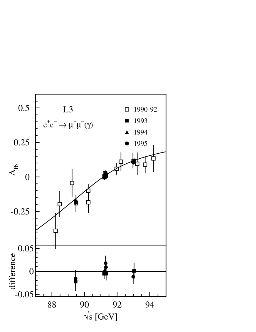
Figure 28: The measured forward-backward asymmetry in $\mathrm{e^{+}e^{-}}\rightarrow\mathrm{\mu^{+}\mu^{-}}(\mathrm{\gamma})$ as function of the centre-of-mass energy. The solid line shows the result of the fit. At the bottom the difference of the measured asymmetry and the fit result for the data collected in $1993-95$ is shown. The errors are statistical only.

Figures 28 to 30 compare these measurements to the results of the fit to all hadronic and leptonic cross section and forward-backward asymmetry measurements imposing lepton universality. For the Bhabha scattering the difference of the forward and backward cross sections in the $s$- and $t$-channels and in the interference, all normalised to the total cross section, are displayed separately. Good agreement between measurements in different years is observed.

For the fits presented in the following sections we include the cross section and forward-backward asymmetry measurements from $1990-92$ [4]. All our measurements at the Z resonance performed in the period $1990-95$ are self-consistent. Qualitatively this can be seen from Figure 31 where for all 175 measurements the absolute difference between the measurements and the expectations, divided by the statistical error of the measurements, is shown. The expected cross sections and forward-backward asymmetries are calculated from the result of the five parameter fit presented in Section 12.3. The scattering of our measurements is compared with the one expected from a perfect Gaussian distribution. The agreement is satisfactory considering that due to their complicated correlations, systematic errors cannot be taken into account in this comparison.

11 Fits for Electroweak Parameters

Different analyses are used to extract electroweak parameters from the measured total cross sections and forward-backward asymmetries.

Firstly, we determine the electroweak parameters making a minimum of assumptions about any underlying theory, for example the SM. The first analysis uses only the total cross section data to determine the parameters of the $\mathrm{Z}$ boson, its mass, the total and partial decay widths to fermion pairs. The second analysis also includes the asymmetry data, which allows the determination of the coupling constants of the neutral weak current. In a third analysis we fit the cross section and forward-backward asymmetry measurements in the S-Matrix ansatz [37] where all contributions from $\mathrm{\gamma}/\mathrm{Z}$-interference are determined from the data. Finally, all our measurements on electroweak observables are interpreted in the framework of the SM in order to determine its free parameters.

Lowest Order Formulae

In all analyses, a Breit-Wigner ansatz is used to describe the $\mathrm{Z}$ boson. The mass, $m_{\mathrm{Z}}$, and the total width, $\Gamma_{\mathrm{Z}}$, of the Z boson are defined by the functional form of the Breit-Wigner denominator, which explicitly takes into account the energy dependence of the total width [38]. The total $s$-channel cross section to lowest order, $\sigma^{\circ}$, for the process $\mathrm{e^{+}e^{-}}\rightarrow\mathrm{f\bar{f}}$, is given by the sum of three terms, the $\mathrm{Z}$ exchange, $\sigma^{\circ}_{\mathrm{Z}}$, the photon exchange, $\sigma^{\circ}_{\gamma}$, and the $\mathrm{\gamma}/\mathrm{Z}$-interference, $\sigma^{\circ}_{\mathrm{int}}$:

$$\sigma^{\circ} = \sigma^{\circ}_{\mathrm{Z}}+\sigma^{\circ}_{\gamma}+\sigma^{\circ}_{\mathrm{int}}$$

$$\sigma^{\circ}_{\mathrm{Z}} = \frac{12\pi}{m_{\mathrm{Z}}^{2}}\frac{\Gamma_{\mathrm{e}}\Gamma_{\mathrm{f}}}{\Gamma_{\mathrm{Z}}^{2}}\frac{s\Gamma_{\mathrm{Z}}^{2}}{(s-m_{\mathrm{Z}}^{2})^{2}+s^{2}\Gamma_{\mathrm{Z}}^{2}/m_{\mathrm{Z}}^{2}}$$

$$\sigma^{\circ}_{\gamma} = \frac{4\pi\alpha^{2}}{3s}q_{\mathrm{e}}^{2}q_{\mathrm{f}}^{2}N_{\mathrm{C}}^{\mathrm{f}}$$

$$\sigma^{\circ}_{\mathrm{int}} = \frac{4\pi\alpha^{2}}{3}J_{\mathrm{f}}\frac{s-m_{\mathrm{Z}}^{2}}{(s-m_{\mathrm{Z}}^{2})^{2}+s^{2}\Gamma_{\mathrm{Z}}^{2}/m_{\mathrm{Z}}^{2}},\qquad\mathrm{f}=\mathrm{e},\,\mu,\,\tau,\,\mathrm{q}$$ (6)

where $q_{\mathrm{f}}$ is the electric charge of the final-state fermion, $N_{\mathrm{C}}^{\mathrm{f}}$ its colour factor, and $\alpha$ the electromagnetic coupling constant. The pure photon exchange is determined by QED.

The first analysis treats the mass and the total and partial widths of the $\mathrm{Z}$ boson as free and independent parameters. The interference of the Z exchange with the photon exchange adds another parameter, the $\mathrm{\gamma}/\mathrm{Z}$-interference term, $J_{\mathrm{f}}$, besides those corresponding to mass and widths of the $\mathrm{Z}$. Since in the SM $|\sigma^{\circ}_{\mathrm{int}}(s)|\ll\sigma^{\circ}(s)$ for centre-of-mass energies close to $m_{\mathrm{Z}}$, it is difficult to measure $J_{\mathrm{f}}$ accurately using data at the $\mathrm{Z}$ only. The $\mathrm{\gamma}/\mathrm{Z}$-interference term is usually taken from the SM [3, 4, 39], thus making assumptions about the form of the electroweak unification.

The second analysis determines the vector and axial-vector coupling constants of the neutral weak current to charged leptons, $g_{\mathrm{V}}^{\ell}$ and $g_{\mathrm{A}}^{\ell}$, by using the forward-backward asymmetries in addition to the total cross sections. In lowest order, for $\sqrt{s}=m_{\mathrm{Z}}$ and neglecting the photon exchange, the $s$-channel forward-backward asymmetry for the process $\mathrm{e^{+}e^{-}}\rightarrow\mathrm{\ell^{+}\ell^{-}}(\mathrm{\gamma})$ is given by:

$$A_{\mathrm{FB}}^{\mathrm{0,\ell}} = \frac{3}{4}A_{\mathrm{e}}A_{\ell}\quad\mathrm{with\ }$$

$$A_{\ell} = \frac{2\,g_{\mathrm{V}}^{\ell}g_{\mathrm{A}}^{\ell}}{(g_{\mathrm{V}}^{\ell})^{2}+(g_{\mathrm{A}}^{\ell})^{2}}\,.$$ (7)

The energy dependence of the asymmetry distinguishes $g_{\mathrm{V}}^{\ell}$ and $g_{\mathrm{A}}^{\ell}$ [40]. The experimental precision on the coupling constants is improved by also including information from tau-polarisation measurements which determine $A_{\mathrm{e}}$ and $A_{\mathrm{\tau}}$ independently.

In Equation 6, the leptonic partial width, $\Gamma_{\ell}$, and the leptonic $\mathrm{\gamma}/\mathrm{Z}$-interference term, $J_{\ell}$, are now expressed in terms of $g_{\mathrm{V}}^{\ell}$ and $g_{\mathrm{A}}^{\ell}$:

$$\Gamma_{\ell} = \frac{G_{\mathrm{F}}m_{\mathrm{Z}}^{3}}{6\sqrt{2}\pi}\left[(g_{\mathrm{V}}^{\ell})^{2}+(g_{\mathrm{A}}^{\ell})^{2}\right]$$

$$J_{\ell} = \frac{G_{\mathrm{F}}m_{\mathrm{Z}}^{2}}{\sqrt{2}\pi\alpha}\,q_{\mathrm{e}}q_{\ell}\,g_{\mathrm{V}}^{\mathrm{e}}g_{\mathrm{V}}^{\ell},$$ (8)

where $G_{\mathrm{F}}$ is the Fermi coupling constant. The hadronic cross section is given by the sum over the five kinematically allowed flavours and their colour states. Because no separation of quark flavours is attempted, this approach cannot be applied to the hadronic final state. Therefore, the parameterisation of the first analysis is used to express the hadronic cross section in terms of $\Gamma_{\mathrm{had}}$ and $J_{\mathrm{had}}$.

Our data are also interpreted in the framework of the S-Matrix ansatz [37], which makes a minimum of theoretical assumptions. This ansatz describes the hard scattering process of fermion-pair production in $\mathrm{e^{+}e^{-}}$-annihilations by the $s$-channel exchange of two spin-1 bosons, a massless photon and a massive $\mathrm{Z}$ boson. The lowest-order total cross section, $\sigma_{\mathrm{tot}}^{0}$, and forward-backward asymmetry, $A^{0}_{\mathrm{FB}}$, for $\mathrm{e^{+}e^{-}}\rightarrow\mathrm{f\bar{f}}$ are given as:

$$\sigma_{\mathrm{a}}^{0}(s) = \frac{4}{3}\pi\alpha^{2}\left[\frac{g_{\mathrm{f}}^{\mathrm{a}}}{s}+\frac{s\,r_{\mathrm{f}}^{\mathrm{a}}+\left(s-\overline{m}_{\mathrm{Z}}^{2}\right)j_{\mathrm{f}}^{\mathrm{a}}}{\left(s-\overline{m}_{\mathrm{Z}}^{2}\right)^{2}+\overline{m}_{\mathrm{Z}}^{2}\overline{\Gamma}_{\mathrm{Z}}^{2}}\right]\qquad\qquad\mathrm{for\ a=tot,FB}$$

$$A^{0}_{\mathrm{FB}}(s) = \frac{3}{4}\frac{\sigma_{\mathrm{FB}}^{0}(s)}{\sigma_{\mathrm{tot}}^{0}(s)}\,.$$ (9)

The S-Matrix parameters $r_{\mathrm{f}}^{\mathrm{a}}$, $j_{\mathrm{f}}^{\mathrm{a}}$ and $g_{\mathrm{f}}^{\mathrm{a}}$ are real numbers which express the size of the $\mathrm{Z}$ exchange, $\mathrm{\gamma}/\mathrm{Z}$-interference  and photon exchange contributions. Here, $r_{\mathrm{f}}^{\mathrm{a}}$ and $j_{\mathrm{f}}^{\mathrm{a}}$ are treated as free parameters while the photon exchange contribution, $g_{\mathrm{f}}^{\mathrm{a}}$, is fixed to its QED prediction. Each final state is thus described by four free parameters: two for cross sections, $r_{\mathrm{f}}^{\mathrm{tot}}$ and $j_{\mathrm{f}}^{\mathrm{tot}}$, and two for forward-backward asymmetries, $r_{\mathrm{f}}^{\mathrm{FB}}$ and $j_{\mathrm{f}}^{\mathrm{FB}}$. In models with only vector and axial-vector couplings of the $\mathrm{Z}$ boson, these four S-Matrix parameters are not independent of each other:

$$r_{\mathrm{f}}^{\mathrm{tot}} \propto \left[(g_{\mathrm{V}}^{\mathrm{e}})^{2}+(g_{\mathrm{A}}^{\mathrm{e}})^{2}\right]\,\left[(g_{\mathrm{V}}^{\mathrm{f}})^{2}+(g_{\mathrm{A}}^{\mathrm{f}})^{2}\right]\,,$$

$$j_{\mathrm{f}}^{\mathrm{tot}} \propto g_{\mathrm{V}}^{\mathrm{e}}g_{\mathrm{V}}^{\mathrm{f}}\,,$$

$$r_{\mathrm{f}}^{\mathrm{FB}} \propto g_{\mathrm{A}}^{\mathrm{e}}g_{\mathrm{V}}^{\mathrm{e}}\,g_{\mathrm{A}}^{\mathrm{f}}g_{\mathrm{V}}^{\mathrm{f}}\,,$$

$$j_{\mathrm{f}}^{\mathrm{FB}} \propto g_{\mathrm{A}}^{\mathrm{e}}g_{\mathrm{A}}^{\mathrm{f}}\,.$$ (10)

Under the assumption that only vector- and axial-vector couplings exist, the S-Matrix ansatz corresponds to the second analysis discussed above without fixing $J_{\mathrm{had}}$ to the SM.

The S-Matrix ansatz is defined using a Breit-Wigner denominator with $s$-independent width for the $\mathrm{Z}$ resonance. To derive the mass and width of the $\mathrm{Z}$ boson for a Breit-Wigner with $s$-dependent width, the following transformations are applied [37]: $m_{\mathrm{Z}}=\overline{m}_{\mathrm{Z}}+34.1\ \mathrm{Me\kern-1.00006ptV}$ and $\Gamma_{\mathrm{Z}}=\overline{\Gamma}_{\mathrm{Z}}+0.9\ \mathrm{Me\kern-1.00006ptV}$.

Radiative Corrections

The QED radiative corrections to the total cross sections and forward-backward asymmetries are included by convolution and by the replacement $\alpha\rightarrow\alpha(s)=\alpha/(1-\Delta\alpha)$ to account for the running of the electromagnetic coupling constant [41, 40].

Weak radiative corrections are calculated assuming the validity of the SM and as a function of the unknown mass of the Higgs boson. The coupling constants which are real to lowest order are modified by absorbing weak corrections and become complex quantities [42]. Effective couplings, $\bar{g}_{\mathrm{V}}^{\mathrm{\ell}}$ and $\bar{g}_{\mathrm{A}}^{\mathrm{\ell}}$, are defined which correspond to the real parts. When extracting $\bar{g}_{\mathrm{V}}^{\mathrm{\ell}}$ and $\bar{g}_{\mathrm{A}}^{\mathrm{\ell}}$ from the measurements, the small imaginary parts are taken from the SM. Observables such as the leptonic partial widths (Equation 8) and the leptonic pole asymmetry (Equation 7) are redefined by replacing the vector and axial-vector coupling constants by these effective couplings.

The effective couplings of fermions are expressed in terms of the effective electroweak mixing angle, $\sin^{2}\!\overline{\theta}_{\mathrm{W}}$, and the effective ratio of the neutral to charged weak current couplings, $\bar{\rho}=1/(1-\Delta\bar{\rho})$ [42]:

$$\bar{g}_{\mathrm{V}}^{\mathrm{f}} = \sqrt{\bar{\rho}}\,(I^{\mathrm{f}}_{3}-2\,q_{\mathrm{f}}\sin^{2}\!\overline{\theta}_{\mathrm{W}})$$

$$\bar{g}_{\mathrm{A}}^{\mathrm{f}} = \sqrt{\bar{\rho}}\,I^{\mathrm{f}}_{3}\,,$$ (11)

where $I^{\mathrm{f}}_{3}$ is the third component of the weak isospin of the fermion f. Due to weak vertex corrections, the definitions of $\bar{\rho}$ and $\sin^{2}\!\overline{\theta}_{\mathrm{W}}$ depend on the fermion. However, except for the b-quark, these differences are small compared to the experimental precision. Therefore, we define $\sin^{2}\!\overline{\theta}_{\mathrm{W}}$ as the effective weak mixing angle for a massless charged lepton. It is related to the on-shell definition of the weak mixing angle, $\sin^{2}\!\theta_{\mathrm{W}}$ by the factor $\kappa$:

$$\kappa=\frac{\sin^{2}\!\overline{\theta}_{\mathrm{W}}}{\sin^{2}\!\theta_{\mathrm{W}}}\qquad\mathrm{with\ }\sin^{2}\!\theta_{\mathrm{W}}=1-\frac{m_{\mathrm{W}}^{2}}{m_{\mathrm{Z}}^{2}}\,.$$ (12)

Fits in the SM

The fourth analysis to determine electroweak parameters uses the framework of the SM. By comparing its predictions with the set of experimental measurements, it is possible to test the consistency of the SM and to constrain the mass of the Higgs boson.

The input parameters of the SM are $\alpha$, the fermion masses, $m_{\mathrm{H}}$, $m_{\mathrm{Z}}$ and the mass of the W boson, $m_{\mathrm{W}}$. QCD adds one more parameter, the strong coupling constant, $\alpha_{\mathrm{s}}$, which is relevant for hadronic final states. The Cabbibo-Kobayashi-Maskawa matrix, relating electroweak and mass eigenstates of quarks, is not important for total hadronic cross sections in neutral current interactions considered here. Concerning the fermion masses, only the mass of the top quark is important for SM calculations performed below. All other masses are too small to play a significant role or are known to sufficient precision.

Generally, in SM calculations for observables at the $\mathrm{Z}$ resonance, the mass of the W is replaced by the Fermi coupling constant, $G_{\mathrm{F}}$, which is measured precisely in muon decay [43]. These two parameters are related by

$$\frac{G_{\mathrm{F}}}{\sqrt{2}}=\frac{\pi\alpha}{2}\,\frac{1}{m_{\mathrm{Z}}^{2}\sin^{2}\!\theta_{\mathrm{W}}\cos^{2}\!\theta_{\mathrm{W}}}\,\\ \frac{1}{1-\Delta r}\,,$$

where $\Delta r$ takes into account the electroweak radiative corrections. These corrections can be split into QED corrections due to the running of the QED coupling constant, $\Delta\alpha$, and pure weak corrections, $\Delta r_{\mathrm{w}}$ [44, 45]:

$$\Delta r = \Delta\alpha+\Delta r_{\mathrm{w}}$$

$$\Delta r_{\mathrm{w}} = -\cot^{2}\!\theta_{\mathrm{W}}\,\Delta\bar{\rho}\,+\Delta r_{\mathrm{rem}}\,.$$ (13)

The corrections $\Delta r_{\mathrm{rem}}$, not absorbed in the $\rho$-parameter, are smaller than the main contributions discussed below but are nevertheless numerically important [46, 45] and included in the calculations.

Weak radiative corrections originate mainly from loop corrections to the W propagator due to the large mass splitting in the top-bottom iso-spin doublet and Higgs boson loop corrections to the propagators of the heavy gauge bosons [47]. To leading order they depend quadratically on $m_{\mathrm{t}}$ and logarithmically on $m_{\mathrm{H}}$. The $\mathrm{Z}\mathrm{b\bar{b}}$ vertex receives additional weak radiative corrections which depend on the top mass. Through the measurements of weak radiative corrections our results at the $\mathrm{Z}$ are sensitive to the mass of the top quark and the Higgs boson. This allows to test the SM at the one-loop level by comparing the top mass derived from our data with the direct measurement and to estimate the mass of the yet undiscovered Higgs boson which is one of the fundamental parameters of the SM. With this procedure the relevant parameters in SM fits are $m_{\mathrm{Z}}$, $m_{\mathrm{t}}$, $m_{\mathrm{H}}$, $\alpha$($m_{\mathrm{Z}}$) and $\alpha_{\mathrm{s}}$.

Fitting Programs and Methods

The programs ZFITTER [48] and TOPAZ0 [49] are used to calculate radiative corrections and SM predictions. For computational reasons the fits are performed using ZFITTER.

Both programs include complete ${\cal O}(\alpha^{2})$ and leading ${\cal O}(\alpha^{3}\ln^{3}(s/m^{2}_{\mathrm{e}}))$ QED calculations of initial state radiation [50]. Final state corrections are calculated in ${\cal O}(\alpha)$ for QED and ${\cal O}(\alpha_{\mathrm{s}}^{3})$ [51] for QCD including also mixed terms ${\cal O}(\alpha\hbox{$\alpha_{\mathrm{s}}$})$. Interference of initial and final state radiation is included up to ${\cal O}(\alpha)$ corrections. Pair production by initial state radiation is implemented [52].

Electroweak radiative corrections are complete at the one-loop level and are supplemented by leading ${\cal O}(G_{\mathrm{F}}^{2}m_{\mathrm{t}}^{4})$ and sub-leading ${\cal O}(G_{\mathrm{F}}^{2}m_{\mathrm{t}}^{2}m_{\mathrm{Z}}^{2})$ [53] two-loop corrections. Complete mixed QCD-electroweak corrections of ${\cal O}(\alpha\hbox{$\alpha_{\mathrm{s}}$})$ with leading ${\cal O}(G_{\mathrm{F}}m_{\mathrm{t}}^{2}\alpha_{s}^{2})$ terms are included [54] together with a non-factorizable part [55].

For the reaction $\mathrm{e^{+}e^{-}}\rightarrow\mathrm{e^{+}e^{-}}(\mathrm{\gamma})$ the contributions from the $t$-channel photon and Z boson exchange and the $s/t$-interference are calculated with the programs ALIBABA [56] and TOPAZ0 (see Appendix A).

Electroweak parameters are determined in $\chi^{2}$ fits using the MINUIT [57] program. The $\chi^{2}$ is constructed from the theoretical expectations, our measurements and their errors, including the correlations. Apart from experimental statistical and systematic errors, and theoretical errors, we take into account uncertainties on the LEP centre-of-mass energy. Technical details of the fit procedure are described in Appendix B.

Theoretical uncertainties on SM predictions of cross sections, asymmetries, Z decay widths and effective coupling constants are studied in detail in Reference [58, 59]. Errors on the theoretical calculations of cross section and forward-backward asymmetries based on total and partial $\mathrm{Z}$ widths, effective couplings or S-Matrix parameters, as used in the fits of Section 12, arise mainly from the finite precision of the QED convolution. They are found to be small compared to the experimental precision and do not introduce sizeable uncertainties in the fit for $\mathrm{Z}$ parameters. Residual SM uncertainties in the imaginary part of the effective couplings are even smaller.

The only exceptions are the theoretical uncertainty on the luminosity determination, discussed in Section 5, and the treatment of $t$-channel and $s/t$-interference contributions to the $\mathrm{e^{+}e^{-}}$ final state due to missing higher order terms and the precision of the ALIBABA program [60]. Uncertainties on the Bhabha cross section and forward-backward asymmetry from calculations of the $t$-channel and $s/t$-interference contributions are discussed in Appendix A.

Additional uncertainties arise in the calculation of SM parameters from the application of different re-normalisation schemes, momentum transfer scales for vertex corrections and factorisations schemes [58]. By comparing different calculations as implemented in ZFITTER and TOPAZ0, we find that the impact of these theoretical uncertainties on the fit results for SM parameters presented in Section 13 is negligible compared to the experimental errors.

ZFITTER and TOPAZ0 calculations in the SM framework are performed based on five input parameters: the masses of the Z and Higgs bosons, the top quark mass, the strong coupling constant $\alpha_{\mathrm{s}}$ at $m_{\mathrm{Z}}$ and the contribution of the five light quark flavours, $\Delta\alpha^{(5)}_{\mathrm{had}}$, to the running of the QED coupling constant to $m_{\mathrm{Z}}$. For comparison to the SM we use the following set of values and uncertainties [61, 62, 63, 64, 34]:

$$\begin{array}[]{r@{$\,=\,$}lr@{$\,=\,$}ll}m_{\mathrm{Z}}&91\,189.8\pm 3.1\ \mathrm{Me\kern-1.00006ptV}\,,&m_{\mathrm{t}}&173.8\pm 5.2\ \mathrm{Ge\kern-1.00006ptV}\,,&95.3\ \mathrm{Ge\kern-1.00006ptV}\leq m_{\mathrm{H}}\leq 1\ \mathrm{Te\kern-1.00006ptV}\,,\\ \Delta\alpha^{(5)}_{\mathrm{had}}&0.02804\pm 0.00065\,,&\hbox{$\alpha_{\mathrm{s}}$}&0.119\pm 0.002\,.\end{array}$$ (14)

The central values are calculated for $m_{\mathrm{H}}=300\ \mathrm{Ge\kern-1.00006ptV}$. This arbitrary choice is motivated by the logarithmic dependence of electroweak observables on $m_{\mathrm{H}}$ and it leads to approximately symmetric theoretical errors.

We use the default settings of ZFITTER which provide the most accurate calculations. Exceptions are that in all calculations we allow for the variation of the contribution of the five light quarks to the running of the QED coupling constant, $\Delta\alpha^{(5)}_{\mathrm{had}}$. Secondly, as recommended by the authors of ZFITTER, the corrections of Reference [55] are explicitly calculated for SM expectations and in fits in the SM framework (Section 13). In all other cases they are absorbed in the definitions of the parameters.

12 Determination of $\mathrm{Z}$  Parameters

12.1 Mass, Total and Partial Widths of the $\mathrm{Z}$

We determine the mass, the total width and the partial decay widths of the $\mathrm{Z}$ into hadrons, electrons, muons and taus in a fit to the measured total cross sections. These parameters describe the contribution of the $\mathrm{Z}$ exchange to the total cross section. The photon exchange and $\mathrm{\gamma}/\mathrm{Z}$-interference contributions are fixed to their SM expectations. Two fits are performed: one assuming and one not assuming lepton universality, where in the first one a common leptonic width is defined as the decay width of the $\mathrm{Z}$ into a pair of massless charged leptons. The results of both fits are summarised in Table 21 and the correlation coefficients for the parameters determined in the two fits are given in Tables 22 and 23, respectively. The partial decay widths into the three charged lepton species are found to be consistent within errors. It should be noted that due to the mass of the tau lepton, $\Gamma_{\tau}$ is expected to be $0.19\ \mathrm{Me\kern-1.00006ptV}$ smaller than $\Gamma_{\ell}$.

Our new results with significantly reduced errors are in agreement with the SM expectations and our previous measurements [4]. For the mass $m_{\mathrm{Z}}$ and the total width $\Gamma_{\mathrm{Z}}$ we obtain:

$$m_{\mathrm{Z}} = 91\,189.8\pm 3.1\ \mathrm{Me\kern-1.00006ptV}\,,$$

$$\Gamma_{\mathrm{Z}} = 2\,502.4\pm 4.2\ \mathrm{Me\kern-1.00006ptV}\,.$$ (15)

These are measurements of the mass of the $\mathrm{Z}$ boson with an accuracy of $3.4\cdot 10^{-5}$ and of its total decay width of $1.7\cdot 10^{-3}$. The contribution to the total errors on $m_{\mathrm{Z}}$ and $\Gamma_{\mathrm{Z}}$ from the LEP energy is estimated by performing fits to the $1993-95$ data with and without taking into account LEP energy errors. From a quadratic subtraction of the errors of the fitted parameters we find $\Delta m_{\mathrm{Z}}(\mathrm{LEP})=1.8\ \mathrm{Me\kern-1.00006ptV}$ and $\Delta\Gamma_{\mathrm{Z}}(\mathrm{LEP})=1.3\ \mathrm{Me\kern-1.00006ptV}$, in agreement with the estimates given in Reference [9].

The impact of the uncertainties on SM parameters on the fit results is negligible. The largest effect is an uncertainty on the $\mathrm{Z}$ mass of $\pm 0.2\ \mathrm{Me\kern-1.00006ptV}$ caused by the calculation of the $\mathrm{\gamma}/\mathrm{Z}$-interference contribution when varying the Higgs and top masses and $\Delta\alpha^{(5)}_{\mathrm{had}}$ in the ranges given in Equation 14.

Motivated by the different methods used to obtain the absolute scale of the LEP energy in the years $1990-92$, $1993-94$ and 1995, resulting in different uncertainties, we determine the mass of the $\mathrm{Z}$ for these three periods independently. The mass values obtained are consistent within their statistical errors.

To check our results on $m_{\mathrm{Z}}$ and $\Gamma_{\mathrm{Z}}$ the fit assuming lepton universality is repeated twice: i) using only the leptonic cross sections and ii) using only the $\mathrm{e^{+}e^{-}}\rightarrow\mathrm{e^{+}e^{-}}(\mathrm{\gamma})$ data. The results for the mass and total width obtained this way are $m_{\mathrm{Z}}=91\,198.7\pm 8.2\ \mathrm{Me\kern-1.00006ptV}$, $\Gamma_{\mathrm{Z}}=2\,508.1\pm 13.4\ \mathrm{Me\kern-1.00006ptV}$ using all three lepton species and $m_{\mathrm{Z}}=91\,177\pm 16\ \mathrm{Me\kern-1.00006ptV}$, $\Gamma_{\mathrm{Z}}=2\,497\pm 26\ \mathrm{Me\kern-1.00006ptV}$ when using only Bhabha scattering data. Within the errors, dominated by the statistical errors of the measurements, these values are in agreement with those given in Table 21 where the $\mathrm{e^{+}e^{-}}\rightarrow\mathrm{hadrons}(\mathrm{\gamma})$ cross section measurements contribute most. Also, we conclude that there is no significant bias introduced in the determination of the mass and the total width of the Z boson by the treatment of the $t$-channel in Bhabha scattering.

From the difference of the total width and the partial widths into hadrons and charged leptons, including their correlations, the decay width of the $\mathrm{Z}$ into invisible particles is derived to be

$$\Gamma_{\mathrm{inv}}=499.1\pm 2.9\ \mathrm{Me\kern-1.00006ptV}\,.$$ (16)

This number is determined in the fit assuming lepton universality and it is in agreement with our direct determination of $\Gamma_{\mathrm{inv}}$ from cross section measurements of the reaction $\mathrm{e^{+}e^{-}}\rightarrow\mathrm{\nu\bar{\nu}}\mathrm{\gamma}(\mathrm{\gamma})$ [65] which yields $\Gamma_{\mathrm{inv}}=498\pm 12\mathrm{(stat)}\pm 12\mathrm{(sys)}\ \mathrm{Me\kern-1.00006ptV}$.

In the SM, the invisible width is exclusively given by the $\mathrm{Z}$ decays into neutrinos and the result can be interpreted as the number of neutrino generations $N_{\mathrm{\nu}}$. Using the SM prediction $\Gamma_{\ell}/\Gamma_{\nu}=0.5021\pm 0.0002$ for the ratio of the $\mathrm{Z}$ decay width into charged leptons and neutrinos we obtain:

$$N_{\mathrm{\nu}}=\frac{\Gamma_{\mathrm{inv}}}{\Gamma_{\ell}}\,\left(\frac{\Gamma_{\ell}}{\Gamma_{\nu}}\right)^{\mathrm{SM}}=2.978\pm 0.014\,.$$ (17)

This formula is used because the experimental precision on the ratio $\Gamma_{\mathrm{inv}}/\Gamma_{\ell}$ is better than that on $\Gamma_{\mathrm{inv}}$.

12.2 Limits on Non-Standard Decays of the $\mathrm{Z}$

From the measurements of total and partial $\mathrm{Z}$ decay widths presented in the previous section we derive experimental limits on additional $\mathrm{Z}$ decay widths not accounted for in the SM. These limits take into account experimental and theoretical errors added in quadrature. The latter are derived from adding in quadrature the changes in the theoretical predictions when varying the SM input parameters by their errors as given in Equation 14. This is motivated by the fact that these parameters are determined in independent experiments with the exception of the mass of the Higgs boson. A value of $m_{\mathrm{H}}=1\ \mathrm{Te\kern-1.00006ptV}$ is used here to calculate the Z widths which results in the lowest SM predictions and therefore in conservative limits.

The 95% confidence level (C.L.) limits on non-standard decay widths, $\Gamma^{\mathrm{NP}}_{\mathrm{95}}$, are calculated using the formula [66]:

$$1-0.95 = \frac{\int_{-\infty}^{\Gamma^{\mathrm{exp}}}\mathrm{d}\Gamma\,G(\Gamma;\Gamma^{\mathrm{SM}}+\Gamma^{\mathrm{NP}}_{\mathrm{95}},\Delta)}{\int_{-\infty}^{\Gamma^{\mathrm{exp}}}\mathrm{d}\Gamma\,G(\Gamma;\Gamma^{\mathrm{SM}},\Delta)}$$

$$\mathrm{with\ }G(\Gamma;\mu,\Delta) = \frac{1}{\sqrt{2\pi}\Delta}\exp{\left[-\frac{(\Gamma-\mu)^{2}}{2\Delta^{2}}\right]}\,,$$ (18)

where $\Gamma^{\mathrm{exp}}$ is our experimental result, $\Gamma^{\mathrm{SM}}$ the SM expectation for $m_{\mathrm{H}}=1\ \mathrm{Te\kern-1.00006ptV}$ and $\Delta$ the combined experimental and theoretical error.

The limits obtained for the total, hadronic, leptonic and invisible widths, as well as for the three lepton species, are summarised in Table 24. Also listed are the differences of our measurements and the SM expectations together with their experimental and theoretical 68% C.L. errors. It should be noted that the results on the total and partial widths are correlated; hence the limits derived in this section cannot be applied simultaneously.

12.3 Fits to Total Cross Sections and Forward-Backward Asymmetries

The measured leptonic forward-backward asymmetries are included in the fits. Besides $m_{\mathrm{Z}}$ and $\Gamma_{\mathrm{Z}}$ the measurements are fitted to the hadronic pole cross section, $\sigma^{0}_{\mathrm{had}}$, the ratios of hadronic to leptonic widths, $R_{\mathrm{\ell}}$, and the leptonic pole asymmetries, $A_{\mathrm{FB}}^{\mathrm{0,\ell}}$, which are defined as:

$$\sigma^{0}_{\mathrm{had}}=\frac{12\pi}{m_{\mathrm{Z}}^{2}}\,\frac{\Gamma_{\mathrm{e}}\Gamma_{\mathrm{had}}}{\Gamma_{\mathrm{Z}}^{2}}\,,\quad R_{\mathrm{\ell}}=\frac{\Gamma_{\mathrm{had}}}{\Gamma_{\ell}}\,,\quad A_{\mathrm{FB}}^{\mathrm{0,\ell}}=\frac{3}{4}\,A_{\mathrm{e}}\,A_{\mathrm{\ell}}\\ \qquad(\ell=\mathrm{e},\,\mu\,,\tau)\,.$$ (19)

The advantage of this parameter set is that the parameters are less correlated than the partial widths. Two fits are performed, one with and one without assuming lepton universality. The results are listed in Table 25 and the correlation matrices are given in Tables 26 and 27.

The 68% C.L. contours in the $A_{\mathrm{FB}}^{\mathrm{0,\ell}}-R_{\mathrm{\ell}}$ plane are derived from these fits for the three lepton species separately and for all leptons combined (Figure 32). In this plot the contour of $A_{\mathrm{FB}}^{\mathrm{0,\tau}}-R_{\mathrm{\tau}}$ is shifted by the difference in expectation for $R_{\mathrm{\tau}}$ due to the tau mass to facilitate the comparison with the other leptons. Also for the forward-backward asymmetries good agreement among the lepton species is observed. Our results are in agreement with the SM expectations.

From the measurements of the forward-backward pole asymmetries the polarisation parameter, $A_{\ell}$, can be derived for the three individual lepton types as well as the average value. The results are listed in Table 28. Because of their relation to the measured pole asymmetry (Equation 7) the results for $A_{\mathrm{e}}$, $A_{\mu}$ and $A_{\tau}$ are highly correlated. They are compared to $A_{\mathrm{e}}$ and $A_{\tau}$ derived from our measurements of the average and the forward-backward tau-polarisation [67]. All measurements are in good agreement and yield an average value of

$$A_{\ell}=0.1575\pm 0.0067\,.$$ (20)

12.4 Vector- and Axial-Vector Coupling Constants of Charged Leptons

The effective coupling constants, $\bar{g}_{\mathrm{V}}^{\mathrm{\ell}}$ and $\bar{g}_{\mathrm{A}}^{\mathrm{\ell}}$, are obtained from a fit to cross section and forward-backward asymmetry measurements, and including our results from tau-polarisation. We use the results from tau-polarisation on $A_{\mathrm{e}}$ and $A_{\tau}$ as given in Table 28 together with a 8% correlation of the errors. The inclusion of tau-polarisation results significantly improves the determination of the effective coupling constants.

Fits with and without assuming lepton universality are performed and the vector and axial-vector coupling constants so obtained are listed Table 29. The axial-vector coupling constant of the electron is taken to be negative, in agreement with the combination of results from neutrino-electron scattering and low energy $A_{\mathrm{FB}}$ measurements [68]. All other signs are unambiguously determined by our measurements.

The 68% C.L. contours in the $\bar{g}_{\mathrm{V}}$-$\bar{g}_{\mathrm{A}}$ plane are shown in Figure 33, revealing good agreement among the three lepton species and thus supporting lepton universality in neutral currents. This is quantified by calculating the ratio of muon and tau to electron coupling constants, taking into account their correlations (see Table 30).

The average vector and axial-vector coupling constants of charged leptons are found to be

$$\bar{g}_{\mathrm{V}}^{\mathrm{\ell}}=-0.0397\pm 0.0017\,,\qquad\bar{g}_{\mathrm{A}}^{\mathrm{\ell}}=-0.50153\pm 0.00053\,.$$ (21)

The resulting axial-vector coupling constant $\bar{g}_{\mathrm{A}}^{\mathrm{\ell}}$ is significantly different from its lowest order SM expectation $-1/2$. This is interpreted as proof for the existence of weak radiative corrections from higher order processes and corresponds to a measurement of the $\rho$-parameter of

$$\bar{\rho}=1.0061\pm 0.0021\,.$$ (22)

The evidence for the existence of weak radiative corrections is illustrated in Figure 33.

Measurements of forward-backward asymmetries and tau-polarisation can be compared in terms of the effective weak mixing angle, $\sin^{2}\!\overline{\theta}_{\mathrm{W}}$, defined by the ratio of the coupling constants (Equation 11). From the average leptonic pole asymmetry and the tau polarisation, the values listed in Table 31 are obtained. Our results obtained from the measurement of the forward-backward asymmetry of b-quarks [69] and the measurement of the quark charge asymmetry, $Q_{\mathrm{FB}}$, [70] are also shown. All four measurements of the weak mixing angle are in agreement with each other and the average yields:

$$\sin^{2}\!\overline{\theta}_{\mathrm{W}}=0.23093\pm 0.00066\,.$$ (23)

12.5 Fits in the S-Matrix Framework

The programs SMATASY [71] together with ZFITTER, ALIBABA and TOPAZ0 are used for the calculation of the theoretical predictions, including QED radiative corrections, of total cross sections and forward-backward asymmetries. Further details can be found in Reference [72].

The results of the fits in the S-Matrix framework with and without imposing lepton universality to the cross sections and forward-backward asymmetries measured at the Z resonance are shown in Table 32. The fitted parameters for electrons, muons, taus and hadrons are in agreement with each other and with the expectations from the SM. The correlations of the parameters as obtained in the two fits are shown in Tables 33 and 34, respectively.

Large correlations among the parameters are observed. Of particular importance is the correlation of $-0.95$ between the mass of the $\mathrm{Z}$ boson and the hadronic interference term, $j^{\mathrm{tot}}_{\mathrm{had}}$. It causes an increase of the error on $m_{\mathrm{Z}}$ with respect to the fits performed in Sections 12.1 and 12.3 where the $\mathrm{\gamma}/\mathrm{Z}$-interference terms are fixed to their SM expectations. The correlation between $m_{\mathrm{Z}}$ and $j^{\mathrm{tot}}_{\mathrm{had}}$ is illustrated in Figure 34.

Comparing the results on the $\mathrm{Z}$ boson mass obtained with the two analyses (Table 21 or 25 and Table 32) good agreement is found. From a quadratic subtraction we estimate the additional error on the $\mathrm{Z}$ mass arising from the experimental uncertainty on the hadronic interference term to be:

$$m_{\mathrm{Z}}=91\,185.2\pm 3.1\pm 9.8(j^{\mathrm{tot}}_{\mathrm{had}})\ \mathrm{Me\kern-1.00006ptV}\,.$$ (24)

The interference between the photon and the $\mathrm{Z}$ is measured to much better precision at centre-of-mass energies below or above the $\mathrm{Z}$ resonance. By adding our measurements of hadronic and leptonic cross sections and forward-backward asymmetries above the $\mathrm{Z}$ resonance this contribution to the error on $m_{\mathrm{Z}}$ is significantly reduced. This will be reported in a forthcoming publication.

13 Results on SM Parameters

We interpret our measurements in the framework of the SM to check its consistency by comparing our results to other measurements. The strategy will be to test at first QCD radiative corrections in terms of $\alpha_{\mathrm{s}}$ before we verify weak radiative corrections by comparing the top mass derived from our data at the $\mathrm{Z}$ resonance to the direct measurement. From our measurements at the $\mathrm{Z}$, the W mass is determined and compared to our result obtained above the W-pair threshold. Finally we use all our measurements of electroweak parameters and include the direct measurement of $m_{\mathrm{t}}$ to estimate the mass of the SM Higgs boson.

Fits are performed to our data to determine the set of SM parameters given in Equation 14. The program ZFITTER is used for SM calculations. In all fits the QED coupling constant at the mass of the $\mathrm{Z}$ is calculated using the constraint on the contribution from the five light quark flavours to the running as obtained in Reference [64].

The input data for the SM fits are our measurements of total cross sections and forward-backward asymmetries at the $\mathrm{Z}$ resonance performed between 1990 and 1995. In addition, our results from tau polarisation (Table 28), the effective weak mixing angles from b-quark forward-backward and form quark charge asymmetry (Table 31), as well as the partial decay width into b-quarks $R_{\mathrm{b}}=\Gamma_{\mathrm{b}}/\Gamma_{\mathrm{had}}=0.2174\pm 0.0032$ [73], are included.

Firstly, the sensitivity of our data to QCD radiative corrections is exploited to determine the strong coupling constant at the mass of the Z boson:

$$\alpha_{\mathrm{s}} = 0.1226\,^{+0.0066}_{-0.0060}\,.$$ (25)

In this fit the result of Section 12.1 is obtained again for $m_{\mathrm{Z}}$ and $\Delta\alpha^{(5)}_{\mathrm{had}}$ remains within the imposed constraint. The masses of the top quark and the Higgs boson are free parameters and their uncertainties are included in the error on $\alpha_{\mathrm{s}}$.

The value for $\alpha_{\mathrm{s}}$ is in good agreement with our determination of the strong coupling constant from hadronic event topologies $\hbox{$\alpha_{\mathrm{s}}$}=0.1216\pm 0.0017\pm 0.0058$ [74]. We use this measurement as an additional constraint and obtain for the top mass:

$$m_{\mathrm{t}}=197\,^{+30}_{-16}\ \mathrm{Ge\kern-1.00006ptV}\,.$$ (26)

This result for the top quark mass is based on our measurements of weak radiative corrections and their interpretation in the SM framework. The agreement with the direct $m_{\mathrm{t}}$ measurements by the CDF and D0 experiments, $m_{\mathrm{t}}=173.8\pm 5.2\ \mathrm{Ge\kern-1.00006ptV}$ [61], means that the bulk of weak radiative corrections indeed originates from the large mass of the top quark. The result for the Higgs boson mass obtained in this fit, $\log_{10}m_{\mathrm{H}}/\mathrm{Ge\kern-1.00006ptV}=1.99\,^{+0.98}_{-0.66}$, is in agreement with the range allowed by the direct search and the SM (Equation 14).

From the result of this fit which is based on measurements at the Z resonance a value for the mass of the W boson is derived:

$$m_{\mathrm{W}}=80.523\pm 0.079\ \mathrm{Ge\kern-1.00006ptV}\,.$$ (27)

The 68% C.L. contour in the $m_{\mathrm{t}}$-$m_{\mathrm{W}}$ plane obtained in this fit is shown in Figure 35. This result for the W mass agrees well with our direct measurements of $m_{\mathrm{W}}$ performed at centre-of-mass energies between $161\ \mathrm{Ge\kern-1.00006ptV}$ and $183\ \mathrm{Ge\kern-1.00006ptV}$ [75, 76, 77] which yield a combined value of $m_{\mathrm{W}}=80.61\pm 0.15\ \mathrm{Ge\kern-1.00006ptV}$.

We include the direct measurement of $m_{\mathrm{W}}$ to determine the electroweak radiative corrections $\Delta r$, the parameters $\rho$ and $\kappa$, the effective weak mixing angle $\sin^{2}\!\overline{\theta}_{\mathrm{W}}$ and the on-shell definition $\sin^{2}\!\theta_{\mathrm{W}}$ as well as a combined result for $m_{\mathrm{W}}$:

$$\begin{array}[]{r@{$\,=\,$}lr@{$\,=\,$}lr@{$\,=\,$}l}\Delta r&0.0257\pm 0.0043\,,&\rho&1.0078\pm 0.0017\,,&\kappa&1.0493\pm 0.0053\,,\\ \sin^{2}\!\overline{\theta}_{\mathrm{W}}&0.23075\pm 0.00054\,,&\sin^{2}\!\theta_{\mathrm{W}}&0.2199\pm 0.0013\,,&m_{\mathrm{W}}&80.541\pm 0.069\ \mathrm{Ge\kern-1.00006ptV}\,.\end{array}$$ (28)

This value for the effective weak mixing angle $\sin^{2}\!\overline{\theta}_{\mathrm{W}}$ derived in a SM fit is in good agreement with the result obtained, in a less model-dependent way, from measurements of asymmetries (Table 31).

Finally, we constrain the mass of the top quark to the combined value from the direct measurement of D0 and CDF. The five SM parameters and their correlations obtained in this fit are summarised in Tables 35 and 36, respectively. In particular, for the mass of the yet undiscovered SM Higgs boson, we obtain a value and an upper limit:

$$m_{\mathrm{H}} = 36^{+43}_{-19}\ \mathrm{Ge\kern-1.00006ptV}\,,$$ (29)

$$< 133\ \mathrm{Ge\kern-1.00006ptV}\qquad 95\%\ \mathrm{C.L.}$$

Figure 36 shows the 68% and 95% C.L. contours in the $m_{\mathrm{t}}$-$m_{\mathrm{H}}$ plane and Figure 37 the dependence of the $\chi^{2}$ of the fit on the Higgs mass from which the upper mass limit is derived. The result is compatible with the result of our direct search for the SM Higgs boson $m_{\mathrm{H}}>95.3\ \mathrm{Ge\kern-1.00006ptV}$ [62].

14 Summary and Conclusion

We report on the precise measurements of total cross sections and forward-backward asymmetries of the reactions $\mathrm{e^{+}e^{-}}\rightarrow\mathrm{hadrons}(\mathrm{\gamma})$, $\mathrm{e^{+}e^{-}}\rightarrow\mathrm{\mu^{+}\mu^{-}}(\mathrm{\gamma})$, $\mathrm{e^{+}e^{-}}\rightarrow\mathrm{\tau^{+}\tau^{-}}(\mathrm{\gamma})$ and $\mathrm{e^{+}e^{-}}\rightarrow\mathrm{e^{+}e^{-}}(\mathrm{\gamma})$ at centre-of-mass energies at the peak and the wings of the $\mathrm{Z}$ resonance performed in the years $1993-95$. A total luminosity of $103\ \mathrm{pb^{-1}}$ corresponding to 2.5 million hadronic and 250 thousand leptonic decays of the $\mathrm{Z}$ was collected which significantly improve our measurements of the resonance curve. Including the data samples collected in previous years, the total number of $\mathrm{Z}$ decays observed by the L3 detector during the first phase of LEP amounts to 4 million which are used to determine the properties of the $\mathrm{Z}$ and other SM parameters.

All our measurements are consistent with the hypothesis of lepton universality. From the measured total hadronic and leptonic cross sections we obtain:

$$m_{\mathrm{Z}}=91\,189.8\pm 3.1\ \mathrm{Me\kern-1.00006ptV}\,, \Gamma_{\mathrm{Z}}=2\,502.4\pm 4.2\ \mathrm{Me\kern-1.00006ptV}\,,$$

$$\Gamma_{\mathrm{had}}=1\,751.1\pm 3.8\ \mathrm{Me\kern-1.00006ptV}\,, \Gamma_{\ell}=84.14\pm 0.17\ \mathrm{Me\kern-1.00006ptV}\,.$$

From these results, the decay width of the $\mathrm{Z}$ into invisible particles is derived to be $\Gamma_{\mathrm{inv}}=499.1\pm 2.9\ \mathrm{Me\kern-1.00006ptV}$, which in the SM corresponds to a number of light neutrino species of:

$$N_{\mathrm{\nu}}=2.978\pm 0.014\,.$$ (30)

Including our measurements of leptonic forward-backward asymmetries and tau polarisation the effective vector and axial-vector coupling constants of charged leptons to the $\mathrm{Z}$ are determined to be:

$$\bar{g}_{\mathrm{V}}^{\mathrm{\ell}}=-0.0397\pm 0.0017\,,\qquad\bar{g}_{\mathrm{A}}^{\mathrm{\ell}}=-0.50153\pm 0.00053\,.$$ (31)

For the effective weak mixing angle we obtain:

$$\sin^{2}\!\overline{\theta}_{\mathrm{W}}=0.23093\pm 0.00066\,,$$ (32)

including our measurements of the b-quark forward-backward and quark charge asymmetries.

Our measurements are sensitive to higher order weak radiative corrections which depend on the masses of the top quark and the Higgs boson. Using in addition our measurements of the partial width $\mathrm{Z}\rightarrow\mathrm{b\bar{b}}$ and $\alpha_{\mathrm{s}}$, we derive in the SM framework a top quark mass

$$m_{\mathrm{t}}=197\,^{+30}_{-16}\ \mathrm{Ge\kern-1.00006ptV}\,,$$ (33)

which is in agreement with the direct measurements of $m_{\mathrm{t}}$. Using our direct measurement of $m_{\mathrm{W}}$ and the knowledge of $m_{\mathrm{t}}$ our data constrain the mass of the Higgs boson to

$$m_{\mathrm{H}}<133\ \mathrm{Ge\kern-1.00006ptV}\qquad 95\%\ \mathrm{C.L.}$$ (34)

Appendix A Treatment of Contributions related to the $t$-channel

In the case of the process $\mathrm{e^{+}e^{-}}\rightarrow\mathrm{e^{+}e^{-}}(\mathrm{\gamma})$, the existence of the $t$-channel exchange of photons and $\mathrm{Z}$ bosons and its interference with the $s$-channel exchange lead to additional complications. Analytical programs to calculate this process, such as ALIBABA and TOPAZ0, are not directly suited for fitting purposes, as computationally they are very time consuming. Thus, the following procedure is adopted. During the initialisation of a fit, ALIBABA is used once to calculate the predictions of the $t$-channel and $s/t$-interference contributions to the measured $\mathrm{e^{+}e^{-}}\rightarrow\mathrm{e^{+}e^{-}}(\mathrm{\gamma})$ cross sections and forward-backward asymmetries. Calculations are performed at several centre-of-mass energy values in the vicinity of the data points allowing for a reduction of the statistical error of the Monte Carlo integration used by ALIBABA and the calculation of derivatives needed to construct the covariance matrix (see Appendix B). ZFITTER is employed during the fits to calculate the corresponding s-channel contributions as a function of the varying electroweak parameters.

The contribution from $s/t$-interference depends on the fit parameter, most importantly on the Z boson mass. This dependence is taken into account by converting the difference between the Z mass used in the initialisation and the current fit value into an equivalent shift in the centre-of-mass energy at which the $t$-channel and $s/t$-interference contributions are calculated. The dependence of the $s/t$-interference on $m_{\mathrm{Z}}$ is responsible for a correlation of the results for $m_{\mathrm{Z}}$ and the electron $s$-channel cross section which amounts to $+11\%$ between $m_{\mathrm{Z}}$ and $R_{\mathrm{e}}$ in the nine parameter fit (Table 26).

In the analytical program ZFITTER polar angular cuts can only be applied on the positron while in the experimental cross section measurements both electron and positron are required to lie within the fiducial volume. Correction factors are calculated with TOPAZ0 which allows for both types of cuts. Finally, cross sections of $\mathrm{e^{+}e^{-}}\rightarrow\mathrm{e^{+}e^{-}}(\mathrm{\gamma})$ to be compared to the experimental measurement are calculated as:

$$\sigma^{\mathrm{th}} = \sigma^{t+s/t,\mathrm{AL}}(44^{\circ}<\theta_{\mathrm{e^{-}}},\theta_{\mathrm{e^{+}}}<136^{\circ})+\sigma^{s,\mathrm{ZF}}(44^{\circ}<\theta_{\mathrm{e^{+}}}<136^{\circ})\,\,R$$

$$\mathrm{with\ }R = \frac{\sigma^{s,\mathrm{T0}}(44^{\circ}<\theta_{\mathrm{e^{-}}},\theta_{\mathrm{e^{+}}}<136^{\circ})}{\sigma^{s,\mathrm{T0}}(44^{\circ}<\theta_{\mathrm{e^{+}}}<136^{\circ})}$$ (35)

All cross sections are defined for an acollinearity angle cut of $\xi<25^{\circ}$. The indices AL, T0 and ZF label cross sections calculated with the ALIBABA, TOPAZ0 and ZFITTER programs, respectively. Cuts on the polar angle of the electron and positron are given in parentheses. This procedure is applied because it combines the most accurate treatment of electroweak radiative corrections as available in ZFITTER and TOPAZ0 with the most complete calculations of $t$-channel contributions in ALIBABA. In the case of the forward-backward asymmetry, $A_{\mathrm{FB}}=(\sigma_{\mathrm{F}}-\sigma_{\mathrm{B}})/(\sigma_{\mathrm{F}}+\sigma_{\mathrm{B}})$, the analogous calculations for the forward, $\sigma_{\mathrm{F}}$, and backward cross sections, $\sigma_{\mathrm{B}}$, are performed.

The cross sections calculated with the ALIBABA and TOPAZ0 programs for all $1990-95$ data sets are listed in in Table 37. The theoretical uncertainties on the calculation of the $t$-channel contributions are listed in Table 38. These errors are applied to the measured cross sections and forward-backward asymmetries in the fits (see Appendix B).

Due to the contribution of the $t$-channel the results from the Bhabha channel cannot be directly compared to the measurements of the other leptonic final states. To permit such a comparison, Equation 35 is used to calculate the $s$-channel contributions, replacing $\sigma^{\mathrm{th}}$ by the measurements and using ZFITTER for the extrapolation to the full solid angle. The $s$-channel cross sections obtained this way, $\sigma^{\mathrm{s}}_{\mathrm{e}}$, without any cuts, and $s$-channel asymmetries, $A_{\mathrm{FB}}^{s}$, with an acollinearity angle cut of $\xi<25^{\circ}$, are given in Tables 17 and 20.

Appendix B Construction of the Covariance Matrix

All fits for electroweak parameters described in this article are performed in the error matrix analysis. They consist of minimising a $\chi^{2}$ function defined as

$$\chi^{2}=D^{T}\,V^{-1}\,D\,,$$ (36)

where $D$ is a column vector with elements defined by the difference between measurements $\Omega_{i}^{\mathrm{exp}}$ and theoretical expectations $\Omega_{i}^{\mathrm{th}}$ which are calculated during the fit as a function of the fit parameters:

$$D_{i}=\Omega_{i}^{\mathrm{exp}}-\Omega_{i}^{\mathrm{th}}\,.$$ (37)

The index $i$ runs over all cross section ($\Omega_{i}=\sigma_{i}$) and forward-backward asymmetry ($\Omega_{i}={A_{\mathrm{FB}}}_{,i}$) measurements considered in the fit. There are 100 cross section and 75 forward-backward asymmetry measurements at the $\mathrm{Z}$ resonance taken in $1990-95$.

The covariance matrix $V$ is constructed in the following way from all experimental and theoretical errors affecting the measurements. The diagonal elements, $V_{ii}$, are obtained adding all individual errors of measurement $i$ in quadrature

$$V_{ii} = \left(f_{i}\,\Delta_{i}^{\mathrm{stat}}\right)^{2}+\left(f_{i}\,\Delta_{i}^{\mathrm{unc}}\right)^{2}+\left(\Delta_{i}^{\mathrm{cor}}\right)^{2}+\left(\Delta_{i}^{\mathrm{abs}}\right)^{2}$$ (38)

$$+V_{ii}^{\mathrm{lum}}+V_{ii}^{\mathrm{LEP}}+V_{ii}^{\epsilon_{\mathrm{cms}}}+V_{ii}^{t}\,,$$

where $\Delta_{i}^{\mathrm{stat}}$ is the statistical error of the measurement, $\Delta_{i}^{\mathrm{unc}}$ the uncorrelated part of the systematic error, $\Delta_{i}^{\mathrm{cor}}=\delta_{i}^{\mathrm{cor}}\,\sigma_{i}^{\mathrm{th}}$ the correlated systematic error which scales with the expected value and $\Delta_{i}^{\mathrm{abs}}$ the correlated part of the systematic error which does not scale. In case of the forward-backward asymmetry the systematic error can simply be expressed in terms of $\Delta_{i}^{\mathrm{abs}}$ only. The statistical and uncorrelated systematic errors which are derived from the measurements (Tables 14 to 20) are scaled during the fit with factors $f_{i}$ to the expected errors using the theoretical expectations:

$$f_{i}=\sqrt{\frac{\sigma_{i}^{\mathrm{th}}}{\sigma_{i}^{\mathrm{exp}}}}\quad(\mathrm{for}\ \sigma_{i})\,,\qquad f_{i}=\sqrt{\frac{1-\left({A_{\mathrm{FB}}}^{\mathrm{th}}_{,i}\right)^{2}}{1-\left({A_{\mathrm{FB}}}^{\mathrm{exp}}_{,i}\right)^{2}}\,\frac{\sigma_{i}^{\mathrm{exp}}}{\sigma_{i}^{\mathrm{th}}}}\quad(\mathrm{for}\ {A_{\mathrm{FB}}}_{,i})\,.$$ (39)

For cross section measurements there is an additional contribution of the luminosity measurement, $V_{ii}^{\mathrm{lum}}$. Its calculation as well as the contribution from the uncertainty on the LEP centre-of-mass energy, $V_{ii}^{\mathrm{LEP}}$, and its spread, $V_{ii}^{\epsilon_{\mathrm{cms}}}$, both applied to cross sections and $A_{\mathrm{FB}}$ measurements, and the theoretical uncertainty on the subtraction of the $t$-channel and $s/t$-interference contribution to Bhabha scattering, $V_{ii}^{t}$, are described below.

The off-diagonal elements are constructed from correlated error sources:

$$V_{ij} = \Delta_{i}^{\mathrm{cor}}\,\Delta_{j}^{\mathrm{cor}}+\Delta_{i}^{\mathrm{abs}}\,\Delta_{j}^{\mathrm{abs}}$$ (40)

$$+V_{ij}^{\mathrm{lum}}+V_{ij}^{\mathrm{LEP}}+V_{ij}^{\epsilon_{\mathrm{cms}}}+V_{ij}^{t}\qquad\qquad(i\neq j)\,.$$

Experimental systematic errors, $\Delta^{\mathrm{cor}}$ and $\Delta^{\mathrm{abs}}$, are only applied to elements connecting the same observable, either cross section or asymmetry, of the same reaction. As above, for forward-backward asymmetry measurements contributions from $\Delta^{\mathrm{cor}}$ and $V^{\mathrm{lum}}$ are not applicable. Contributions from $V_{ij}^{\mathrm{lum}}$, $V_{ij}^{\mathrm{LEP}}$, $V_{ij}^{\epsilon_{\mathrm{cms}}}$ and $V_{ij}^{t}$ enter also into off-diagonal elements connecting measurements of different observables or reactions.

All statistical errors and the individual contributions to systematic errors for the measurements performed in $1993-95$ are listed in Tables 14 to 20. For the measurements performed in $1990-92$ systematic errors are quoted in Reference [4] as relative errors, $\delta_{i}$, for the cross section and absolute errors, $\Delta_{i}$, for the forward-backward asymmetries. The correlation among these systematic errors is treated by using $V_{ij}=(\min(\delta_{i},\delta_{j}))^{2}\,\sigma_{i}^{\mathrm{th}}\sigma_{j}^{\mathrm{th}}$ for the cross sections and $V_{ij}=(\min(\Delta_{i},\Delta_{j}))^{2}$ for the asymmetries. Contributions from uncertainties on the luminosity and the LEP energy are added, where applicable.

Correlations between experimental systematic errors in the $1990-92$ and $1993-95$ data sets are estimated in the same way by using the smaller values of $1993-95$. Exceptions are the measurements of the $\mathrm{e^{+}e^{-}}\rightarrow\mathrm{\tau^{+}\tau^{-}}(\mathrm{\gamma})$ cross section where due to the completely revised analysis in $1993-95$ an additional factor of $0.72$ is applied to $\delta_{i}^{\mathrm{cor}}$. Other contributions to elements connecting measurements of $1990-92$ and $1993-95$ are from $V_{ij}^{\epsilon_{\mathrm{cms}}}$, $V_{ij}^{t}$ and the theoretical uncertainty in $V_{ij}^{\mathrm{lum}}$.

Uncertainty on the Luminosity

For the $1993-95$ cross sections the contributions to the covariance matrix from errors on the luminosity measurement are obtained from the sum of the total experimental errors, including their correlations, and the theoretical uncertainty:

$$V_{ij}^{\mathrm{lum}}=\left(\delta_{k}^{\mathrm{lum,exp}}\,\sigma_{i}^{\mathrm{th}}\right)\,\left(\delta_{l}^{\mathrm{lum,exp}}\,\sigma_{j}^{\mathrm{th}}\right)\,\rho_{kl}^{\mathrm{lum,exp}}+\left(\delta_{m}^{\mathrm{lum,stat}}\right)^{2}\,\sigma_{i}^{\mathrm{th}}\sigma_{j}^{\mathrm{th}}+\left(\delta^{\mathrm{lum,th}}\right)^{2}\,\sigma_{i}^{\mathrm{th}}\sigma_{j}^{\mathrm{th}}\,.$$ (41)

The indices $k$ and $l$ label the years of the data sets $i$ and $j$. Total experimental errors on the luminosity, $\delta^{\mathrm{lum,exp}}$, are given in Table 4 and their correlations, $\rho_{kl}^{\mathrm{lum,exp}}$, in Table 5. The statistical error on the luminosity measurement, $\delta^{\mathrm{lum,stat}}$, is given in Table 6 for the nine data taking periods. It applies only to cross section measurements $i$ and $j$ performed in the same period $m$.

The combined experimental and theoretical error on the luminosity determination in $1990-92$ is $\delta^{\mathrm{lum}}=6$. It is treated as fully correlated and the corresponding terms in the covariance matrix are calculated as $V_{ij}^{\mathrm{lum}}=(\delta^{\mathrm{lum}})^{2}\,\sigma_{i}^{\mathrm{th}}\sigma_{j}^{\mathrm{th}}$. For the $1990-92$ data the statistical error of the luminosity measurement is included in the quoted statistical errors of the hadron cross section measurements and it is neglected for the leptonic cross sections. The theoretical uncertainty, $\delta^{\mathrm{lum,th}}=0.61$, is fully correlated among all cross section measurements in $1990-95$.

The measurement of the luminosity, and hence of $\sigma_{i}^{\mathrm{exp}}$, depends on the centre-of-mass energy $E$ due to the approximate $1/E^{2}$ dependence of the Bhabha cross section:

$$\frac{\mathrm{d}\sigma_{i}^{\mathrm{exp}}}{\mathrm{d}E}=-\kappa_{m}\frac{\sigma_{i}^{\mathrm{exp}}}{E_{i}}\,.$$ (42)

Because of the $\mathrm{\gamma}/\mathrm{Z}$-interference and higher order contributions the exponent $\kappa_{m}$ differs from 2 and it is calculated with BHLUMI to be $\kappa_{m}=1.95,\ 2.27$ and $1.97$ for the peak$-2$, peak and peak$+2$ data sets, respectively. This dependence causes a small contribution to the uncertainty on the cross section measurements and it is taken into account for the $1993-95$ data together with the error on the LEP energy.

Uncertainty on the Centre-of-Mass Energy

The errors on the LEP centre-of-mass energy are transformed into equivalent errors of cross section and asymmetry measurements using the partial derivatives of the theoretical cross sections and forward-backward asymmetries with respect to the centre-of-mass energy, $\partial\Omega_{i}^{\mathrm{th}}/\partial E$. The dependence of the measured cross section, via the luminosity, on the centre-of-mass energy is included where applicable.

For the $1993-95$ data sets the terms in the covariance matrix are determined as

$$V_{ij}^{\mathrm{LEP}} = v_{kl}^{\mathrm{LEP}}\,\frac{\mathrm{d}\Omega_{i}}{\mathrm{d}E}\,\frac{\mathrm{d}\Omega_{j}}{\mathrm{d}E}\,,$$

$$\mathrm{with\ }\frac{\mathrm{d}\Omega_{i}}{\mathrm{d}E} = -\frac{\partial\sigma_{i}^{\mathrm{th}}}{\partial E}-\kappa_{m}\frac{\sigma_{i}^{\mathrm{exp}}}{E_{i}}\qquad\mathrm{for\ 1993-95\ cross\ sections,}$$ (43)

$$= -\frac{\partial\Omega_{i}^{\mathrm{th}}}{\partial E}\hskip 76.82243pt\mathrm{otherwise.}$$

where $k$ and $l$ are the indices of the LEP energy calibration periods corresponding to the data sets $i$ and $j$, with $\kappa_{m}$ the appropriate factor defined in Eq. 42. For a pair of data sets taken in any of the seven periods with precise LEP energy calibration, $v_{kl}^{\mathrm{LEP}}$ is the corresponding element of the LEP energy error matrix as given in Table 1. For data sets taken during the 1993 or 1995 pre-scans the LEP energy error is treated as uncorrelated with any other period. Hence, only elements connecting data sets taken during the same pre-scan receive contributions $v_{kk}^{\mathrm{LEP}}=(\delta_{k}^{\mathrm{LEP}})^{2}$, where $\delta_{k}^{\mathrm{LEP}}$ are the uncertainties on the centre-of-mass energy of $18\ \mathrm{Me\kern-1.00006ptV}$ and $10\ \mathrm{Me\kern-1.00006ptV}$ in 1993 and 1995, respectively.

The uncertainties on the LEP centre-of-mass energy in $1990-92$ are listed in Table 3. They are uncorrelated to the energy errors in $1993-95$.

The correction factors for cross sections, $f^{i}_{\epsilon_{\mathrm{cms}}}$, and the absolute corrections for forward-backward asymmetries, $\alpha^{i}_{\epsilon_{\mathrm{cms}}}$, applied to the measurements to account for the spread of the centre-of-mass energy, $\epsilon_{\mathrm{cms}}$, can be calculated to sufficient precision from Taylor expansions:

$$f^{i}_{\epsilon_{\mathrm{cms}}}=1-\frac{1}{2}\frac{1}{\sigma_{i}^{\mathrm{th}}}\frac{\partial^{2}\sigma_{i}^{\mathrm{th}}}{\partial E^{2}}\,\epsilon_{\mathrm{cms}}^{2}\,,\qquad\alpha^{i}_{\epsilon_{\mathrm{cms}}}=-\frac{1}{2}\left[\frac{\partial^{2}{A_{\mathrm{FB}}}^{\mathrm{th}}_{,i}}{\partial E^{2}}+2\,\frac{1}{\sigma_{i}^{\mathrm{th}}}\frac{\partial\sigma_{i}^{\mathrm{th}}}{\partial E}\frac{\partial{A_{\mathrm{FB}}}^{\mathrm{th}}_{,i}}{\partial E}\right]\,\epsilon_{\mathrm{cms}}^{2}\,.$$ (44)

The contributions to the covariance matrix from the uncertainty on the centre-of-mass energy spread, $\Delta\epsilon_{\mathrm{cms}}$, are then given by

$$V_{ij}^{\epsilon_{\mathrm{cms}}} = \Delta_{i}^{\epsilon_{\mathrm{cms}}}\Delta_{j}^{\epsilon_{\mathrm{cms}}}$$

$$\mathrm{with\ }\Delta_{i}^{\epsilon_{\mathrm{cms}}} = 2\,\sigma_{i}^{\mathrm{th}}\,\left(f^{i}_{\epsilon_{\mathrm{cms}}}-1\right)\,\frac{\Delta\epsilon_{\mathrm{cms}}}{\epsilon_{\mathrm{cms}}}\qquad\,\ \mathrm{for\ cross\ sections}\,,$$ (45)

$$= 2\,\alpha^{i}_{\epsilon_{\mathrm{cms}}}\,\frac{\Delta\epsilon_{\mathrm{cms}}}{\epsilon_{\mathrm{cms}}}\qquad\qquad\qquad\quad\mathrm{for\ A_{\mathrm{FB}}}\,.$$

The spread of the centre-of-mass energy and its error for the $1993-95$ data sets are given in Table 2. The centre-of-mass energy spread used in Reference [4] for the $1990-92$ data has been revised and the values and errors given in Reference [9] are used. The error on the centre-of-mass energy spread is fully correlated between all data sets of $1990-95$, hence all elements of the covariance matrix receive a contribution.

Error on $t$-channel Contributions

The last term in Equations 38 and 40 applies to $\mathrm{e^{+}e^{-}}\rightarrow\mathrm{e^{+}e^{-}}(\mathrm{\gamma})$ cross section and $A_{\mathrm{FB}}$ measurements only. It accounts for the uncertainty on the calculation of $t$-channel and $s/t$-interference contributions:

$$V_{ij}^{t}=\Delta_{k}^{t}\,\Delta_{l}^{t}\,.$$ (46)

The indices $k$ and $l$ refer to the centre-of-mass energies of the data set $i$ and $j$ and the corresponding errors on cross sections and asymmetries, $\Delta^{\mathrm{t}}$, are listed in Table 38 [60]. Off-diagonal elements receive a contribution only if the two data sets are both below, on or above the peak. Cross section and asymmetry measurements are also connected this way.

Constraints

In fits using other results, $\Omega_{m}^{\mathrm{c}}$, than cross section and $A_{\mathrm{FB}}$ measurements these additional measurements are added with their errors, $\Delta_{m}^{\mathrm{c}}$, to the $\chi^{2}$ function. This applies to our measurements of tau-polarisation, b-quark and quark charge asymmetries, $R_{\mathrm{b}}$ and $\alpha_{\mathrm{s}}$, as well as to the value of $\Delta\alpha^{(5)}_{\mathrm{had}}$ and the measurement of $m_{\mathrm{t}}$ used in SM fits. Statistical and systematic errors are added in quadrature to obtain $\Delta_{m}^{\mathrm{c}}$:

$$\chi^{2}=D^{T}\,V^{-1}\,D+\sum_{m}\left(\frac{\Omega_{m}^{\mathrm{c}}-\Omega_{m}^{\mathrm{th}}}{\Delta_{m}^{\mathrm{c}}}\right)^{2}\,.$$ (47)

The small correlation of 8% between $A_{\mathrm{e}}$ and $A_{\tau}$ measured from tau-polarisation is included by means of a covariance matrix.

The L3 Collaboration:

M.Acciarri,²⁶ P.Achard,¹⁹ O.Adriani,¹⁶ M.Aguilar-Benitez,²⁵ J.Alcaraz,²⁵ G.Alemanni,²² J.Allaby,¹⁷ A.Aloisio,²⁸ M.G.Alviggi,²⁸ G.Ambrosi,¹⁹ H.Anderhub,⁴⁸ V.P.Andreev,^6,36 T.Angelescu,¹² F.Anselmo,⁹ A.Arefiev,²⁷ T.Azemoon,³ T.Aziz,¹⁰ P.Bagnaia,³⁵ L.Baksay,⁴³ A.Balandras,⁴ R.C.Ball,³ S.Banerjee,¹⁰ Sw.Banerjee,¹⁰ A.Barczyk,^48,46 R.Barillère,¹⁷ L.Barone,³⁵ P.Bartalini,²² M.Basile,⁹ R.Battiston,³² A.Bay,²² F.Becattini,¹⁶ U.Becker,¹⁴ F.Behner,⁴⁸ L.Bellucci,¹⁶ J.Berdugo,²⁵ P.Berges,¹⁴ B.Bertucci,³² B.L.Betev,⁴⁸ S.Bhattacharya,¹⁰ M.Biasini,³² A.Biland,⁴⁸ J.J.Blaising,⁴ S.C.Blyth,³³ G.J.Bobbink,² A.Böhm,¹ L.Boldizsar,¹³ B.Borgia,³⁵ D.Bourilkov,⁴⁸ M.Bourquin,¹⁹ S.Braccini,¹⁹ J.G.Branson,³⁹ V.Brigljevic,⁴⁸ F.Brochu,⁴ I.C.Brock,³³ A.Buffini,¹⁶ A.Buijs,⁴⁴ J.D.Burger,¹⁴ W.J.Burger,³² A.Button,³ X.D.Cai,¹⁴ M.Campanelli,⁴⁸ M.Capell,¹⁴ G.Cara Romeo,⁹ G.Carlino,²⁸ A.M.Cartacci,¹⁶ J.Casaus,²⁵ G.Castellini,¹⁶ F.Cavallari,³⁵ N.Cavallo,³⁷ C.Cecchi,³² M.Cerrada,²⁵ F.Cesaroni,²³ M.Chamizo,¹⁹ Y.H.Chang,⁵⁰ U.K.Chaturvedi,¹⁸ M.Chemarin,²⁴ A.Chen,⁵⁰ G.Chen,⁷ G.M.Chen,⁷ H.F.Chen,²⁰ H.S.Chen,⁷ G.Chiefari,²⁸ L.Cifarelli,³⁸ F.Cindolo,⁹ C.Civinini,¹⁶ I.Clare,¹⁴ R.Clare,¹⁴ G.Coignet,⁴ A.P.Colijn,² N.Colino,²⁵ S.Costantini,⁵ F.Cotorobai,¹² B.Cozzoni,⁹ B.de la Cruz,²⁵ A.Csilling,¹³ S.Cucciarelli,³² T.S.Dai,¹⁴ J.A.van Dalen,³⁰ R.D’Alessandro,¹⁶ R.de Asmundis,²⁸ P.Déglon,¹⁹ A.Degré,⁴ K.Deiters,⁴⁶ D.della Volpe,²⁸ P.Denes,³⁴ F.DeNotaristefani,³⁵ A.De Salvo,⁴⁸ M.Diemoz,³⁵ D.van Dierendonck,² F.Di Lodovico,⁴⁸ C.Dionisi,³⁵ M.Dittmar,⁴⁸ A.Dominguez,³⁹ A.Doria,²⁸ M.T.Dova,^18,♯ D.Duchesneau,⁴ D.Dufournaud,⁴ P.Duinker,² I.Duran,⁴⁰ S.Dutta,¹⁰ H.El Mamouni,²⁴ A.Engler,³³ F.J.Eppling,¹⁴ F.C.Erné,² P.Extermann,¹⁹ M.Fabre,⁴⁶ R.Faccini,³⁵ M.A.Falagan,²⁵ S.Falciano,^35,17 A.Favara,¹⁷ J.Fay,²⁴ O.Fedin,³⁶ M.Felcini,⁴⁸ T.Ferguson,³³ F.Ferroni,³⁵ H.Fesefeldt,¹ E.Fiandrini,³² J.H.Field,¹⁹ F.Filthaut,¹⁷ P.H.Fisher,¹⁴ I.Fisk,³⁹ G.Forconi,¹⁴ L.Fredj,¹⁹ K.Freudenreich,⁴⁸ C.Furetta,²⁶ Yu.Galaktionov,^27,14 S.N.Ganguli,¹⁰ P.Garcia-Abia,⁵ M.Gataullin,³¹ S.S.Gau,¹¹ S.Gentile,^35,17 N.Gheordanescu,¹² S.Giagu,³⁵ Z.F.Gong,²⁰ G.Grenier,²⁴ O.Grimm,⁴⁸ M.W.Gruenewald,⁸ M.Guida,³⁸ R.van Gulik,² V.K.Gupta,³⁴ A.Gurtu,¹⁰ L.J.Gutay,⁴⁵ D.Haas,⁵ A.Hasan,²⁹ D.Hatzifotiadou,⁹ T.Hebbeker,⁸ A.Hervé,¹⁷ P.Hidas,¹³ J.Hirschfelder,³³ H.Hofer,⁴⁸ G. Holzner,⁴⁸ H.Hoorani,³³ S.R.Hou,⁵⁰ I.Iashvili,⁴⁷ V.Innocente,¹⁷ B.N.Jin,⁷ L.W.Jones,³ P.de Jong,² I.Josa-Mutuberría,²⁵ R.A.Khan,¹⁸ M.Kaur,^18,♢ M.N.Kienzle-Focacci,¹⁹ D.Kim,³⁵ J.K.Kim,⁴² J.Kirkby,¹⁷ D.Kiss,¹³ W.Kittel,³⁰ A.Klimentov,^14,27 A.C.König,³⁰ E.Koffeman,² A.Kopp,⁴⁷ V.Koutsenko,^14,27 M.Kräber,⁴⁸ R.W.Kraemer,³³ W.Krenz,¹ A.Krüger,⁴⁷ H.Kuijten,³⁰ A.Kunin,^14,27 P.Ladron de Guevara,²⁵ I.Laktineh,²⁴ G.Landi,¹⁶ K.Lassila-Perini,⁴⁸ M.Lebeau,¹⁷ A.Lebedev,¹⁴ P.Lebrun,²⁴ P.Lecomte,⁴⁸ P.Lecoq,¹⁷ P.Le Coultre,⁴⁸ H.J.Lee,⁸ J.M.Le Goff,¹⁷ R.Leiste,⁴⁷ E.Leonardi,³⁵ P.Levtchenko,³⁶ C.Li,²⁰ S.Likhoded,⁴⁷ C.H.Lin,⁵⁰ W.T.Lin,⁵⁰ F.L.Linde,² L.Lista,²⁸ Z.A.Liu,⁷ W.Lohmann,⁴⁷ E.Longo,³⁵ Y.S.Lu,⁷ W.Lu,³¹ K.Lübelsmeyer,¹ C.Luci,^17,35 D.Luckey,¹⁴ L.Lugnier,²⁴ L.Luminari,³⁵ W.Lustermann,⁴⁸ W.G.Ma,²⁰ M.Maity,¹⁰ L.Malgeri,¹⁷ A.Malinin,¹⁷ C.Maña,²⁵ D.Mangeol,³⁰ P.Marchesini,⁴⁸ G.Marian,¹⁵ J.P.Martin,²⁴ F.Marzano,³⁵ G.G.G.Massaro,² K.Mazumdar,¹⁰ R.R.McNeil,⁶ S.Mele,¹⁷ L.Merola,²⁸ M.Merk,³³ M.Meschini,¹⁶ W.J.Metzger,³⁰ M.von der Mey,¹ A.Mihul,¹² H.Milcent,¹⁷ G.Mirabelli,³⁵ J.Mnich,¹⁷ G.B.Mohanty,¹⁰ P.Molnar,⁸ B.Monteleoni,^16,† T.Moulik,¹⁰ G.S.Muanza,²⁴ F.Muheim,¹⁹ A.J.M.Muijs,² M.Musy,³⁵ M.Napolitano,²⁸ F.Nessi-Tedaldi,⁴⁸ H.Newman,³¹ T.Niessen,¹ A.Nisati,³⁵ H.Nowak,⁴⁷ G.Organtini,³⁵ A.Oulianov,²⁷ C.Palomares,²⁵ D.Pandoulas,¹ S.Paoletti,^35,17 A.Paoloni,³⁵ P.Paolucci,²⁸ R.Paramatti,³⁵ H.K.Park,³³ I.H.Park,⁴² G.Pascale,³⁵ G.Passaleva,¹⁷ S.Patricelli,²⁸ T.Paul,¹¹ M.Pauluzzi,³² C.Paus,¹⁷ F.Pauss,⁴⁸ D.Peach,¹⁷ M.Pedace,³⁵ S.Pensotti,²⁶ D.Perret-Gallix,⁴ B.Petersen,³⁰ D.Piccolo,²⁸ F.Pierella,⁹ M.Pieri,¹⁶ P.A.Piroué,³⁴ E.Pistolesi,²⁶ V.Plyaskin,²⁷ M.Pohl,¹⁹ V.Pojidaev,^27,16 H.Postema,¹⁴ J.Pothier,¹⁷ N.Produit,¹⁹ D.O.Prokofiev,⁴⁵ D.Prokofiev,³⁶ J.Quartieri,³⁸ G.Rahal-Callot,^48,17 M.A.Rahaman,¹⁰ P.Raics,¹⁵ N.Raja,¹⁰ R.Ramelli,⁴⁸ P.G.Rancoita,²⁶ A.Raspereza,⁴⁷ G.Raven,³⁹ P.Razis,²⁹D.Ren,⁴⁸ M.Rescigno,³⁵ S.Reucroft,¹¹ T.van Rhee,⁴⁴ S.Riemann,⁴⁷ K.Riles,³ A.Robohm,⁴⁸ J.Rodin,⁴³ B.P.Roe,³ L.Romero,²⁵ A.Rosca,⁸ S.Rosier-Lees,⁴ S.Roth,¹ J.A.Rubio,¹⁷ D.Ruschmeier,⁸ H.Rykaczewski,⁴⁸ S.Saremi,⁶ S.Sarkar,³⁵ J.Salicio,¹⁷ E.Sanchez,¹⁷ M.P.Sanders,³⁰ M.E.Sarakinos,²¹ C.Schäfer,¹⁷ V.Schegelsky,³⁶ S.Schmidt-Kaerst,¹ D.Schmitz,¹ H.Schopper,⁴⁹ D.J.Schotanus,³⁰ G.Schwering,¹ C.Sciacca,²⁸ D.Sciarrino,¹⁹ A.Seganti,⁹ L.Servoli,³² S.Shevchenko,³¹ N.Shivarov,⁴¹ V.Shoutko,²⁷ E.Shumilov,²⁷ A.Shvorob,³¹ T.Siedenburg,¹ D.Son,⁴² B.Smith,³³ P.Spillantini,¹⁶ M.Steuer,¹⁴ D.P.Stickland,³⁴ A.Stone,⁶ H.Stone,^34,† B.Stoyanov,⁴¹ A.Straessner,¹ K.Sudhakar,¹⁰ G.Sultanov,¹⁸ L.Z.Sun,²⁰ H.Suter,⁴⁸ J.D.Swain,¹⁸ Z.Szillasi,^43,¶ T.Sztaricskai,^43,¶ X.W.Tang,⁷ L.Tauscher,⁵ L.Taylor,¹¹ B.Tellili,²⁴ C.Timmermans,³⁰ Samuel C.C.Ting,¹⁴ S.M.Ting,¹⁴ S.C.Tonwar,¹⁰ J.Tóth,¹³ C.Tully,¹⁷ K.L.Tung,⁷Y.Uchida,¹⁴ J.Ulbricht,⁴⁸ U.Uwer,¹⁷ E.Valente,³⁵ G.Vesztergombi,¹³ I.Vetlitsky,²⁷ D.Vicinanza,³⁸ G.Viertel,⁴⁸ S.Villa,¹¹ M.Vivargent,⁴ S.Vlachos,⁵ I.Vodopianov,³⁶ H.Vogel,³³ H.Vogt,⁴⁷ I.Vorobiev,²⁷ A.A.Vorobyov,³⁶ A.Vorvolakos,²⁹ M.Wadhwa,⁵ W.Wallraff,¹ M.Wang,¹⁴ X.L.Wang,²⁰ Z.M.Wang,²⁰ A.Weber,¹ M.Weber,¹ P.Wienemann,¹ H.Wilkens,³⁰ S.X.Wu,¹⁴ S.Wynhoff,¹⁷ L.Xia,³¹ Z.Z.Xu,²⁰ B.Z.Yang,²⁰ C.G.Yang,⁷ H.J.Yang,⁷ M.Yang,⁷ J.B.Ye,²⁰ S.C.Yeh,⁵¹ J.M.You,³³ An.Zalite,³⁶ Yu.Zalite,³⁶ Z.P.Zhang,²⁰ G.Y.Zhu,⁷ R.Y.Zhu,³¹ A.Zichichi,^9,17,18 G.Zilizi,^43,¶ M.Zöller.¹

• I. Physikalisches Institut, RWTH, D-52056 Aachen, FRG^§
  III. Physikalisches Institut, RWTH, D-52056 Aachen, FRG^§

• National Institute for High Energy Physics, NIKHEF, and University of Amsterdam, NL-1009 DB Amsterdam, The Netherlands

• University of Michigan, Ann Arbor, MI 48109, USA

• Laboratoire d’Annecy-le-Vieux de Physique des Particules, LAPP,IN2P3-CNRS, BP 110, F-74941 Annecy-le-Vieux CEDEX, France

• Institute of Physics, University of Basel, CH-4056 Basel, Switzerland

• Louisiana State University, Baton Rouge, LA 70803, USA

• Institute of High Energy Physics, IHEP, 100039 Beijing, China^△

• Humboldt University, D-10099 Berlin, FRG^§

• University of Bologna and INFN-Sezione di Bologna, I-40126 Bologna, Italy

• Tata Institute of Fundamental Research, Bombay 400 005, India

• Northeastern University, Boston, MA 02115, USA

• Institute of Atomic Physics and University of Bucharest, R-76900 Bucharest, Romania

• Central Research Institute for Physics of the Hungarian Academy of Sciences, H-1525 Budapest 114, Hungary^‡

• Massachusetts Institute of Technology, Cambridge, MA 02139, USA

• KLTE-ATOMKI, H-4010 Debrecen, Hungary^¶

• INFN Sezione di Firenze and University of Florence, I-50125 Florence, Italy

• European Laboratory for Particle Physics, CERN, CH-1211 Geneva 23, Switzerland

• World Laboratory, FBLJA Project, CH-1211 Geneva 23, Switzerland

• University of Geneva, CH-1211 Geneva 4, Switzerland

• Chinese University of Science and Technology, USTC, Hefei, Anhui 230 029, China^△

• SEFT, Research Institute for High Energy Physics, P.O. Box 9, SF-00014 Helsinki, Finland

• University of Lausanne, CH-1015 Lausanne, Switzerland

• INFN-Sezione di Lecce and Universitá Degli Studi di Lecce, I-73100 Lecce, Italy

• Institut de Physique Nucléaire de Lyon, IN2P3-CNRS,Université Claude Bernard, F-69622 Villeurbanne, France

• Centro de Investigaciones Energéticas, Medioambientales y Tecnologícas, CIEMAT, E-28040 Madrid, Spain${\flat}$

• INFN-Sezione di Milano, I-20133 Milan, Italy

• Institute of Theoretical and Experimental Physics, ITEP, Moscow, Russia

• INFN-Sezione di Napoli and University of Naples, I-80125 Naples, Italy

• Department of Natural Sciences, University of Cyprus, Nicosia, Cyprus

• University of Nijmegen and NIKHEF, NL-6525 ED Nijmegen, The Netherlands

• California Institute of Technology, Pasadena, CA 91125, USA

• INFN-Sezione di Perugia and Universitá Degli Studi di Perugia, I-06100 Perugia, Italy

• Carnegie Mellon University, Pittsburgh, PA 15213, USA

• Princeton University, Princeton, NJ 08544, USA

• INFN-Sezione di Roma and University of Rome, “La Sapienza”, I-00185 Rome, Italy

• Nuclear Physics Institute, St. Petersburg, Russia

• INFN-Sezione di Napoli and University of Potenza, I-85100 Potenza, Italy

• University and INFN, Salerno, I-84100 Salerno, Italy

• University of California, San Diego, CA 92093, USA

• Dept. de Fisica de Particulas Elementales, Univ. de Santiago, E-15706 Santiago de Compostela, Spain

• Bulgarian Academy of Sciences, Central Lab. of Mechatronics and Instrumentation, BU-1113 Sofia, Bulgaria

• Laboratory of High Energy Physics, Kyungpook National University, 702-701 Taegu, Republic of Korea

• University of Alabama, Tuscaloosa, AL 35486, USA

• Utrecht University and NIKHEF, NL-3584 CB Utrecht, The Netherlands

• Purdue University, West Lafayette, IN 47907, USA

• Paul Scherrer Institut, PSI, CH-5232 Villigen, Switzerland

• DESY, D-15738 Zeuthen, FRG

• Eidgenössische Technische Hochschule, ETH Zürich, CH-8093 Zürich, Switzerland

• University of Hamburg, D-22761 Hamburg, FRG

• National Central University, Chung-Li, Taiwan, China

• Department of Physics, National Tsing Hua University, Taiwan, China

• Supported by the German Bundesministerium für Bildung, Wissenschaft, Forschung und Technologie

• Supported by the Hungarian OTKA fund under contract numbers T019181, F023259 and T024011.

• Also supported by the Hungarian OTKA fund under contract numbers T22238 and T026178.

• Supported also by the Comisión Interministerial de Ciencia y Tecnología.

• Also supported by CONICET and Universidad Nacional de La Plata, CC 67, 1900 La Plata, Argentina.

• Also supported by Panjab University, Chandigarh-160014, India.

• Supported by the National Natural Science Foundation of China.

• Deceased.

		1993			1994	1995
		peak$-2$	peak	peak$+2$	peak	peak$-2$	peak	peak$+2$
	peak$-2$	$12.59$	$8.32$	$7.45$	$5.59$	$2.05$	$1.80$	$1.84$
1993	peak		$45.69$	$7.68$	$6.20$	$1.69$	$1.82$	$1.72$
	peak$+2$			$9.57$	$5.20$	$1.90$	$1.96$	$2.15$
1994	peak				$14.30$	$1.90$	$2.07$	$1.92$
	peak$-2$					$4.49$	$2.34$	$2.30$
1995	peak						$30.40$	$2.60$
	peak$+2$							$4.15$

Table 1: The covariance matrix, $v_{kl}^{\mathrm{LEP}}$, of the LEP centre-of-mass energy uncertainty at the L3 interaction point for the 1994 data set and the two scans of the Z resonance performed in 1993 and 1995 [9]. All values are given in units of $\mathrm{Me\kern-1.00006ptV}^{2}$.

	$\epsilon_{\mathrm{cms}}$ [$\mathrm{Me\kern-1.00006ptV}$]
	1993	1994	1995
pre-scan	56.8		56.9
peak$-2$	56.6		55.9
peak	57.0	56.5	56.4
peak$+2$	57.1		56.9
$\Delta\epsilon_{\mathrm{cms}}$ [$\mathrm{Me\kern-1.00006ptV}$]	$\pm 1.1$	$\pm 1.1$	$\pm 1.3$

Table 2: The spread on the average centre-of-mass energy, $\epsilon_{\mathrm{cms}}$, and its error, $\Delta\epsilon_{\mathrm{cms}}$, at the L3 interaction point [9] for the nine data sets. The additional scatter from the time variation of the mean centre-of-mass energies is included. The uncertainty does not depend on the energy.

	1990							1991								1992
$\sqrt{s}\ [\mathrm{Ge\kern-0.90005ptV}]$	88.231	89.236	90.238	91.230	92.226	93.228	94.223	91.254	88.480	89.470	90.228	91.222	91.967	92.966	93.716	91.294
88.231	696	675	676	677	678	678	679	0	159	154	150	145	141	136	132	0
89.236		696	682	685	688	691	694	0	151	148	145	142	140	137	135	0
90.238			706	692	698	703	709	0	142	141	141	140	139	139	138	0
91.230				702	708	715	723	0	133	135	136	137	139	140	141	0
92.226					743	728	738	0	125	128	131	135	138	142	145	0
93.228						764	753	0	116	122	126	133	137	143	148	0
94.223							788	0	107	115	122	130	136	145	151	0
91.254								333	0	0	0	0	0	0	0	0
88.480									93.5	61.6	54.1	44.3	36.9	27.1	19.7	0
89.470										74.8	48.2	40.6	34.9	27.3	21.6	0
90.228											66.7	37.8	33.4	27.5	23.0	0
91.222												45.3	31.4	27.7	24.9	0
91.967													53.2	27.9	26.3	0
92.966														45.7	28.3	0
93.716															57.6	0
91.294																324

Table 3: The covariance matrix of the LEP centre-of-mass energy uncertainty for the $1990-92$ data sets obtained following references [31]. All values are given in units of $\mathrm{Me\kern-0.90005ptV}^{2}$. The centre-of-mass energies listed correspond to our measurements in Reference [4].

Source	1993	1994	1995
Selection Criteria []	$0.48$	$0.42$	$0.47$
Detector Geometry []	$0.63$	$0.34$	$0.34$
Monte Carlo Statistics []	$0.35$	$0.35$	$0.35$
Total Experimental ($\delta_{k}^{\mathrm{lum,exp}}$) []	$0.86$	$0.64$	$0.68$
Theory ($\delta_{k}^{\mathrm{lum,th}}$) []	$0.61$	$0.61$	$0.61$
Total Uncertainty []	$1.05$	$0.88$	$0.91$

Table 4: Experimental and theoretical contributions to the systematic error on the luminosity measurement for different years. Additional contributions to the error from statistics and from the uncertainty on the centre-of-mass energy are also taken into account in the fitting procedure.

	1993	1994	1995
1993	1.00	0.59	0.59
1994		1.00	0.93
1995			1.00

Table 5: Correlation coefficients, $\rho_{kl}^{\mathrm{lum,exp}}$, between the data sets of different years of the total experimental systematic error on the luminosity measurement, $\delta_{k}^{\mathrm{lum,exp}}$, as given in Table 4.

		$N_{\mathrm{events}}$	$\delta^{\mathrm{lum,stat}}$ []
1993	pre-scan	$362\,500$	$1.66$
	peak$-2$	$604\,535$	$1.29$
	peak	$651\,931$	$1.24$
	peak$+2$	$588\,962$	$1.30$
1994	peak	$3\,129\,424$	$0.57$
1995	pre-scan	$480\,342$	$1.44$
	peak$-2$	$541\,580$	$1.36$
	peak	$283\,887$	$1.88$
	peak$+2$	$554\,371$	$1.34$
peak combined		$4\,908\,084$	$0.45$

Table 6: Number of events used for the measurement of the total luminosity in the nine data taking periods, $N_{\mathrm{events}}$, and the corresponding contributions to the error of cross section measurements, $\delta^{\mathrm{lum,stat}}$. The numbers correspond to the luminosity used for the hadron cross section measurements and are used for leptonic channels too. The last line is the sum of the five data sets taken at the peak, indicating this error contribution to the measurements of the pole cross sections.

Source	$1993-1995$
Monte Carlo statistics []	$0.04-0.10$
Acceptance []	$0.21$
Selection cuts []	$0.30$
Trigger []	$0.12$
Total scale []	$0.39-0.40$
Non-resonant background [$\mathrm{pb}$]	$3$
Detector noise [$\mathrm{pb}$]	$1$
Total absolute [$\mathrm{pb}$]	$3.2$

Table 7: Contributions to the systematic uncertainty on the cross section $\mathrm{e^{+}e^{-}}\rightarrow\mathrm{hadrons}(\mathrm{\gamma})$. Except for the contribution from Monte Carlo statistics all errors are fully correlated among the data sets. The resulting correlated scale error is $\delta^{\mathrm{cor}}=0.39$.

Source	1993	1994	1995
Monte Carlo statistics []	$0.9-1.5$	$0.4$	$1.7-2.4$
Acceptance []	$2.7$	$2.7$	$3.2$
Selection cuts []	$1.3$	$1.3$	$1.4-2.2$
Trigger []	$0.6$	$0.6$	$0.5-0.7$
Resonant background []	$0.3$	$0.3$	$0.3$
Total scale []	$3.2-3.4$	$3.1$	$3.9-4.6$
$\mathrm{\mathrm{e^{+}e^{-}}\rightarrow\mathrm{e^{+}e^{-}}\,\mathrm{\mu^{+}\mu^{-}}}$ [$\mathrm{pb}$]	$-$	$-$	$0.1$
Cosmic rays [$\mathrm{pb}$]	$0.3$	$0.3$	$0.3$
Total absolute [$\mathrm{pb}$]	$0.3$	$0.3$	$0.3$

Table 8: Contributions to the systematic uncertainty on the cross section $\mathrm{e^{+}e^{-}}\rightarrow\mathrm{\mu^{+}\mu^{-}}(\mathrm{\gamma})$. Except for the contribution from Monte Carlo statistics, all errors are fully correlated among the data sets yielding a correlated scale error of $\delta^{\mathrm{cor}}=3.1$ for $1993-94$ data. For the 1995 data this error is estimated to be $3.6$ and it is taken to be fully correlated with the other years.

Source	$1993-94$	1995
Fit procedure	$<0.0003$	$<0.0003$
Detector asymmetry	$0.0006$	$0.0006$
Charge confusion	$0.0004$	$0.0010$
Momentum reconstruction	$0.0004$	$0.0009$
Background	$0.0001-0.0005$	$<0.0003$
Total uncertainty	$0.0008-0.0009$	$0.0015$

Table 9: Contributions to the systematic uncertainty on the forward-backward asymmetry in $\mathrm{e^{+}e^{-}}\rightarrow\mathrm{\mu^{+}\mu^{-}}(\mathrm{\gamma})$. The total uncertainty is assumed to be fully correlated among the data sets.

Source	1993	1994	1995
Monte Carlo statistics []	$2.3-4.2$	$1.1$	$1.5-1.7$
Tau branching fractions []	$2.0$	$2.0$	$2.0$
Selection cuts []	$5.3-8.0$	$6.0$	$6.4-7.5$
Trigger []	$0.2$	$0.2$	$0.2$
Resonant background []	$1.4-3.3$	$1.0$	$1.3-3.0$
Total scale []	$6.8-9.5$	$6.5$	$7.5-8.0$
$\mathrm{e^{+}e^{-}}\rightarrow\mathrm{e^{+}e^{-}}\,\mathrm{\tau^{+}\tau^{-}},\,\mathrm{e^{+}e^{-}}\,\mathrm{hadrons}$ [$\mathrm{pb}$]	$0.6$
Cosmic rays [$\mathrm{pb}$]	$1.0$
Total absolute [$\mathrm{pb}$]	$1.2$

Table 10: Contributions to the systematic uncertainty on the cross section $\mathrm{e^{+}e^{-}}\rightarrow\mathrm{\tau^{+}\tau^{-}}(\mathrm{\gamma})$. The total absolute and $5.7$ of the total scale error are assumed to be fully correlated among all data sets.

Source	$1993-1995$
Detector asymmetry	$0.0030$
Charge confusion	$<0.0001$
Background	$0.0010$
Helicity bias	$0.0004$
Total uncertainty	$0.0032$

Table 11: Contributions to the systematic uncertainty on the forward-backward asymmetry in $\mathrm{e^{+}e^{-}}\rightarrow\mathrm{\tau^{+}\tau^{-}}(\mathrm{\gamma})$. The total uncertainty is assumed to be fully correlated among the data sets.

Source	1993	1994	1995
Monte Carlo statistics []	$0.4-1.0$	$0.4$	$0.4$
∗ Generator []	$1.0$	$1.0$	$1.0$
∗ $\mathrm{e}$-$\mathrm{\gamma}$ discrimination []	$0.6$	$0.6$	$1.5$
∗ z-vertex position []	$0.5$	$0.5$	$-$
∗ BGO geometry []	$0.5$	$0.5$	$-$
∗ fiducial volume []	$-$	$-$	$1.5$
Background []	$0.7-1.0$	$0.4$	$0.4$
Selection cuts []	$1.6-2.7$	$0.8$	$1.5$
Total scale []	$2.3-3.2$	$1.7$	$2.8$

Table 12: Contributions to the systematic uncertainty on the cross section $\mathrm{e^{+}e^{-}}\rightarrow\mathrm{e^{+}e^{-}}(\mathrm{\gamma})$. Error sources indicated as ^∗ are correlated yielding a total correlated scale error of $\delta^{\mathrm{cor}}=1.4$ for the $1993-94$ data and $2.3$ for the 1995 data.

Source	$1993-1995$
Charge confusion	$0.0020$
$z$-vertex	$0.0015$
Background	$0.0005$
Total uncertainty	$0.0025$

Table 13: Contributions to the systematic uncertainty on the forward-backward asymmetry in $\mathrm{e^{+}e^{-}}\rightarrow\mathrm{e^{+}e^{-}}(\mathrm{\gamma})$.

$\sqrt{s}\ [\mathrm{Ge\kern-1.00006ptV}]$	$N_{\mathrm{events}}$	${\cal L}\ [\mathrm{pb^{-1}}]$	$\sigma\ [\mathrm{nb}]$		$\Delta_{i}^{\mathrm{unc}}\ [\mathrm{nb}]$
$91.3217$	$158\,736$	$5.21$	$30.665$$\,\pm\,$	$0.077$	$0.003$
$89.4498$	$83\,681$	$8.32$	$10.087$$\,\pm\,$	$0.035$	$0.001$
$91.2057$	$281\,359$	$9.34$	$30.309$$\,\pm\,$	$0.057$	$0.003$
$93.0352$	$121\,926$	$8.79$	$13.909$$\,\pm\,$	$0.040$	$0.001$
1993 Totals	$645\,702$	$31.66$
$91.2202$	$1\,359\,490$	$44.84$	$30.513$$\,\pm\,$	$0.026$	$0.001$
$91.3093$	$209\,195$	$6.90$	$30.512$$\,\pm\,$	$0.066$	$0.003$
$89.4517$	$75\,102$	$7.46$	$10.081$$\,\pm\,$	$0.037$	$0.001$
$91.2958$	$123\,791$	$4.08$	$30.493$$\,\pm\,$	$0.086$	$0.003$
$92.9827$	$117\,555$	$8.28$	$14.232$$\,\pm\,$	$0.041$	$0.001$
1995 Totals	$525\,643$	$26.72$
Total sum	$2\,530\,835$	$103.21$

Table 14: Average centre-of-mass energies, number of selected events, integrated luminosities and measured cross sections with statistical errors for $\mathrm{e^{+}e^{-}}\rightarrow\mathrm{hadrons}(\mathrm{\gamma})$. The cross sections are quoted for $\sqrt{s^{\prime}}>0.1\sqrt{s}$. Apart from the uncorrelated part listed, $\Delta_{i}^{\mathrm{unc}}$, systematic errors consist in addition of a fully correlated multiplicative contribution, $\delta_{i}^{\mathrm{cor}}=0.39$ and an absolute uncertainty, $\Delta_{i}^{\mathrm{abs}}=3.2\ \mathrm{pb}$. Systematic errors from the luminosity measurement (Tables 4 and 6) have to be added.

$\sqrt{s}\ [\mathrm{Ge\kern-1.00006ptV}]$	$N_{\mathrm{events}}$	${\cal L}\ [\mathrm{pb^{-1}}]$	$\sigma\ [\mathrm{nb}]$		$\Delta_{i}^{\mathrm{unc}}\ [\mathrm{nb}]$
$91.3216$	$5\,134$	$5.00$	$1.504$$\,\pm\,$	$0.021$	$0.002$
$89.4499$	$2\,739$	$8.03$	$0.504$$\,\pm\,$	$0.010$	$0.001$
$91.2056$	$9\,237$	$9.15$	$1.482$$\,\pm\,$	$0.016$	$0.001$
$93.0357$	$3\,679$	$7.97$	$0.684$$\,\pm\,$	$0.011$	$0.001$
1993 Totals	$20\,789$	$30.15$
$91.2197$	$41\,768$	$41.38$	$1.484$$\,\pm\,$	$0.007$	$0.001$
$91.3090$	$5\,772$	$5.09$	$1.467$$\,\pm\,$	$0.020$	$0.003$
$89.4517$	$2\,789$	$7.36$	$0.490$$\,\pm\,$	$0.009$	$0.001$
$91.2949$	$3\,967$	$3.47$	$1.483$$\,\pm\,$	$0.024$	$0.003$
$92.9825$	$4\,305$	$7.83$	$0.703$$\,\pm\,$	$0.011$	$0.002$
1995 Totals	$16\,833$	$23.75$
Total sum	$79\,390$	$95.29$

Table 15: Same as Table 14 for $\mathrm{e^{+}e^{-}}\rightarrow\mathrm{\mu^{+}\mu^{-}}(\mathrm{\gamma})$. The cross sections are extrapolated to the full phase space. Apart from the uncorrelated part listed, systematic errors consist in addition of a fully correlated multiplicative contribution, $\delta_{i}^{\mathrm{cor}}=3.1$ (3.6 for 1995 data), and an absolute uncertainty, $\Delta_{i}^{\mathrm{abs}}=0.3\ \mathrm{pb}$.

$\sqrt{s}\ [\mathrm{Ge\kern-1.00006ptV}]$	$N_{\mathrm{events}}$	${\cal L}\ [\mathrm{pb^{-1}}]$	$\sigma\ [\mathrm{nb}]$		$\Delta_{i}^{\mathrm{unc}}\ [\mathrm{nb}]$
$91.3221$	$4\,805$	$5.08$	$1.492$$\,\pm\,$	$0.021$	$0.006$
$89.4500$	$2\,706$	$8.08$	$0.509$$\,\pm\,$	$0.010$	$0.004$
$91.2058$	$8\,506$	$9.00$	$1.474$$\,\pm\,$	$0.017$	$0.007$
$93.0358$	$3\,637$	$7.93$	$0.718$$\,\pm\,$	$0.012$	$0.003$
1993 Totals	$19\,654$	$30.09$
$91.2197$	$41\,439$	$43.53$	$1.472$$\,\pm\,$	$0.007$	$0.005$
$91.3096$	$7\,314$	$7.75$	$1.474$$\,\pm\,$	$0.017$	$0.007$
$89.4518$	$2\,352$	$7.48$	$0.483$$\,\pm\,$	$0.010$	$0.002$
$91.2951$	$3\,509$	$3.67$	$1.503$$\,\pm\,$	$0.025$	$0.009$
$92.9828$	$3\,723$	$8.25$	$0.707$$\,\pm\,$	$0.012$	$0.004$
1995 Totals	$16\,898$	$27.15$
Total sum	$77\,991$	$100.77$

Table 16: Same as Table 14 for $\mathrm{e^{+}e^{-}}\rightarrow\mathrm{\tau^{+}\tau^{-}}(\mathrm{\gamma})$. The cross sections are extrapolated to the full phase space. Apart from the uncorrelated part listed, systematic errors consist in addition of a fully correlated multiplicative contribution, $\delta_{i}^{\mathrm{cor}}=5.7$ and an absolute uncertainty, $\Delta_{i}^{\mathrm{abs}}=1.2\ \mathrm{pb}$.

$\sqrt{s}\ [\mathrm{Ge\kern-1.00006ptV}]$	$N_{\mathrm{events}}$	${\cal L}\ [\mathrm{pb^{-1}}]$	$\sigma\ [\mathrm{nb}]$		$\Delta_{i}^{\mathrm{unc}}\ [\mathrm{nb}]$	$\sigma^{s}\ [\mathrm{nb}]$
$91.3213$	$5\,267$	$5.19$	$1.017$$\,\pm\,$	$0.014$	$0.003$	$1.438$$\,\pm\,$	$0.023$
$89.4497$	$4\,610$	$8.28$	$0.566$$\,\pm\,$	$0.008$	$0.001$	$0.515$$\,\pm\,$	$0.014$
$91.2057$	$9\,834$	$9.23$	$1.075$$\,\pm\,$	$0.011$	$0.002$	$1.497$$\,\pm\,$	$0.018$
$93.0358$	$3\,610$	$8.39$	$0.431$$\,\pm\,$	$0.007$	$0.001$	$0.703$$\,\pm\,$	$0.012$
1993 Totals	$23\,321$	$31.09$
$91.2197$	$43\,300$	$40.64$	$1.075$$\,\pm\,$	$0.005$	$0.001$	$1.501$$\,\pm\,$	$0.008$
$91.3106$	$8\,200$	$7.88$	$1.042$$\,\pm\,$	$0.012$	$0.002$	$1.476$$\,\pm\,$	$0.019$
$89.4517$	$3\,891$	$6.91$	$0.564$$\,\pm\,$	$0.009$	$0.001$	$0.511$$\,\pm\,$	$0.015$
$91.2960$	$4\,310$	$4.02$	$1.072$$\,\pm\,$	$0.017$	$0.002$	$1.520$$\,\pm\,$	$0.027$
$92.9828$	$3\,405$	$7.90$	$0.427$$\,\pm\,$	$0.007$	$0.001$	$0.696$$\,\pm\,$	$0.012$
1995 Totals	$19\,806$	$26.72$
Total sum	$86\,427$	$98.45$

Table 17: Average centre-of-mass energies, number of selected events, integrated luminosity and measured cross sections with their statistical and uncorrelated systematic errors in the fiducial volume $44^{\circ}<\theta<136^{\circ}$ and for $\xi<25^{\circ}$ for the reaction $\mathrm{e^{+}e^{-}}\rightarrow\mathrm{e^{+}e^{-}}(\mathrm{\gamma})$. The systematic error consists in addition of a fully correlated multiplicative contribution, $\delta_{i}^{\mathrm{cor}}=1.4$ (2.3 in 1995). In the rightmost column the $s$-channel contribution to the total cross section in the full solid angle is listed with the statistical error (see Appendix A).

$\sqrt{s}\ [\mathrm{Ge\kern-1.00006ptV}]$	$N_{\mathrm{events}}$	$A_{\mathrm{FB}}$
$91.3217$	$5\,385$	$0.009$$\,\pm\,$	$0.015$
$89.4497$	$2\,631$	$-0.182$$\,\pm\,$	$0.020$
$91.2054$	$9\,150$	$0.000$$\,\pm\,$	$0.011$
$93.0352$	$3\,635$	$0.119$$\,\pm\,$	$0.017$
$91.2203$	$43\,416$	$0.0086$$\,\pm\,$	$0.0051$
$91.3090$	$5\,643$	$0.022$$\,\pm\,$	$0.013$
$89.4517$	$2\,686$	$-0.175$$\,\pm\,$	$0.019$
$91.2949$	$3\,858$	$0.030$$\,\pm\,$	$0.016$
$92.9825$	$4\,193$	$0.104$$\,\pm\,$	$0.015$

Table 18: Results on the forward-backward asymmetry, including an acollinearity cut $\xi<15^{\circ}$, for $\mathrm{e^{+}e^{-}}\rightarrow\mathrm{\mu^{+}\mu^{-}}(\mathrm{\gamma})$ together with the average centre-of-mass energies and the number of events. The errors are statistical only and a correlated absolute systematic error of $\Delta_{i}^{\mathrm{abs}}=0.0008$ ($0.0015$ for 1995 data) has to be added.

$\sqrt{s}\ [\mathrm{Ge\kern-1.00006ptV}]$	$N_{\mathrm{events}}$	$A_{\mathrm{FB}}$
$91.3221$	$3\,655$	$-0.003$$\,\pm\,$	$0.017$
$89.4500$	$2\,090$	$-0.138$$\,\pm\,$	$0.022$
$91.2058$	$6\,669$	$0.020$$\,\pm\,$	$0.013$
$93.0358$	$2\,822$	$0.133$$\,\pm\,$	$0.019$
$91.2202$	$36\,509$	$0.0062$$\,\pm\,$	$0.0053$
$91.3096$	$6\,317$	$0.044$$\,\pm\,$	$0.013$
$89.4518$	$2\,020$	$-0.134$$\,\pm\,$	$0.023$
$91.2951$	$3\,017$	$0.001$$\,\pm\,$	$0.018$
$92.9828$	$3\,263$	$0.134$$\,\pm\,$	$0.017$

Table 19: Same as Table 18 for $\mathrm{e^{+}e^{-}}\rightarrow\mathrm{\tau^{+}\tau^{-}}(\mathrm{\gamma})$. The cut on the acollinearity angle is $\xi<10^{\circ}$. The errors are statistical only and a correlated absolute systematic error of $\Delta_{i}^{\mathrm{abs}}=0.0032$ has to be added.

$\sqrt{s}\ [\mathrm{Ge\kern-1.00006ptV}]$	$N_{\mathrm{events}}$	$A_{\mathrm{FB}}$		$A_{\mathrm{FB}}^{s}$
$91.3213$	$4\,009$	$0.083$$\,\pm\,$	$0.016$	$-0.027$$\,\pm\,$	$0.022$
$89.4497$	$3\,434$	$0.311$$\,\pm\,$	$0.016$	$-0.119$$\,\pm\,$	$0.039$
$91.2057$	$7\,330$	$0.111$$\,\pm\,$	$0.012$	$-0.003$$\,\pm\,$	$0.016$
$93.0358$	$2\,679$	$0.101$$\,\pm\,$	$0.019$	$0.110$$\,\pm\,$	$0.024$
$91.2197$	$31\,636$	$0.1213$$\,\pm\,$	$0.0056$	$0.014$$\,\pm\,$	$0.008$
$91.3106$	$7\,861$	$0.101$$\,\pm\,$	$0.011$	$-0.001$$\,\pm\,$	$0.016$
$89.4517$	$3\,722$	$0.257$$\,\pm\,$	$0.016$	$-0.244$$\,\pm\,$	$0.039$
$91.2960$	$4\,083$	$0.080$$\,\pm\,$	$0.016$	$-0.030$$\,\pm\,$	$0.023$
$92.9828$	$3\,203$	$0.055$$\,\pm\,$	$0.018$	$0.054$$\,\pm\,$	$0.022$

Table 20: Measured forward-backward asymmetry in the fiducial volume $44^{\circ}<\theta<136^{\circ}$ and for $\xi<25^{\circ}$ for the reaction $\mathrm{e^{+}e^{-}}\rightarrow\mathrm{e^{+}e^{-}}(\mathrm{\gamma})$. The errors are statistical only and a correlated absolute systematic error of $\Delta_{i}^{\mathrm{abs}}=0.0025$ has to be added. In the rightmost column the $s$-channel contribution to the forward-backward asymmetry in the full solid angle is listed for $\xi<25^{\circ}$ with the statistical error (see Appendix A).

Parameter	Treatment of Charged Leptons				Standard
	non-universality		universality		Model
$m_{\mathrm{Z}}$ [$\mathrm{Me\kern-1.00006ptV}$]	91 189.7$\,\pm\,$	3.1	$91\,189.8$$\,\pm\,$	$3.1$	—
$\Gamma_{\mathrm{Z}}$ [$\mathrm{Me\kern-1.00006ptV}$]	2 502.4$\,\pm\,$	4.2	$2\,502.4$$\,\pm\,$	$4.2$	$2\,492.7\,^{+3.8}_{-5.2}$
$\Gamma_{\mathrm{had}}$ [$\mathrm{Me\kern-1.00006ptV}$]	1 750.9$\,\pm\,$	4.7	$1\,751.1$$\,\pm\,$	$3.8$	$1\,739.8\,^{+3.2}_{-4.1}$
$\Gamma_{\mathrm{e}}$ [$\mathrm{Me\kern-1.00006ptV}$]	84.16$\,\pm\,$	0.22	—		$83.91\,^{+0.10}_{-0.14}$
$\Gamma_{\mu}$ [$\mathrm{Me\kern-1.00006ptV}$]	83.95$\,\pm\,$	0.44	—		$83.91\,^{+0.10}_{-0.14}$
$\Gamma_{\tau}$ [$\mathrm{Me\kern-1.00006ptV}$]	84.23$\,\pm\,$	0.58	—		$83.72\,^{+0.10}_{-0.14}$
$\Gamma_{\ell}$ [$\mathrm{Me\kern-1.00006ptV}$]	—		$84.14$$\,\pm\,$	$0.17$	$83.91\,^{+0.10}_{-0.14}$
$\chi^{2}$/dof	$91/94$		$91/96$		—

Table 21: Results of the fits to the $1990-95$ total cross section data with and without assuming lepton universality.

	$m_{\mathrm{Z}}$	$\Gamma_{\mathrm{Z}}$	$\Gamma_{\mathrm{had}}$	$\Gamma_{\mathrm{e}}$	$\Gamma_{\mu}$	$\Gamma_{\tau}$
$m_{\mathrm{Z}}$	$\phantom{-}1.00$	$\phantom{-}0.06$	$\phantom{-}0.14$	$-0.03$	$\phantom{-}0.07$	$\phantom{-}0.05$
$\Gamma_{\mathrm{Z}}$		$1.00$	$0.54$	$0.55$	$0.28$	$0.21$
$\Gamma_{\mathrm{had}}$			$1.00$	$-0.29$	$0.48$	$0.36$
$\Gamma_{\mathrm{e}}$				$1.00$	$-0.14$	$-0.11$
$\Gamma_{\mu}$					$1.00$	$0.19$
$\Gamma_{\tau}$						$1.00$

Table 22: Correlation matrix for the six parameter fit without assuming lepton universality in Table 21.

	$m_{\mathrm{Z}}$	$\Gamma_{\mathrm{Z}}$	$\Gamma_{\mathrm{had}}$	$\Gamma_{\ell}$
$m_{\mathrm{Z}}$	$\phantom{-}1.00$	$\phantom{-}0.07$	$\phantom{-}0.12$	$\phantom{-}0.03$
$\Gamma_{\mathrm{Z}}$		$1.00$	$0.68$	$0.71$
$\Gamma_{\mathrm{had}}$			$1.00$	$0.12$
$\Gamma_{\ell}$				$1.00$

Table 23: Correlation matrix for the four parameter fit assuming lepton universality in Table 21.

	$\Gamma^{\mathrm{exp}}-\Gamma^{\mathrm{SM}}\ [\mathrm{Me\kern-1.00006ptV}]$			$\Gamma^{\mathrm{NP}}_{\mathrm{95}}\ [\mathrm{Me\kern-1.00006ptV}]$
$\Gamma_{\mathrm{Z}}$	$14.6$$\,\pm\,$	$4.2$ $\,\pm\,$	$1.7$	$22.0$
$\Gamma_{\mathrm{had}}$	$15.2$$\,\pm\,$	$3.8$ $\,\pm\,$	$1.5$	$21.9$
$\Gamma_{\mathrm{inv}}$	$-1.7$$\,\pm\,$	$2.9$ $\,\pm\,$	$0.23$	$4.8$
$\Gamma_{\ell}$	$0.37$$\,\pm\,$	$0.17$ $\,\pm\,$	$0.05$	$0.66$
$\Gamma_{\mathrm{e}}$	$0.38$$\,\pm\,$	$0.22$ $\,\pm\,$	$0.05$	$0.75$
$\Gamma_{\mu}$	$0.17$$\,\pm\,$	$0.44$ $\,\pm\,$	$0.05$	$0.99$
$\Gamma_{\tau}$	$0.64$$\,\pm\,$	$0.58$ $\,\pm\,$	$0.05$	$1.64$

Table 24: The one-sided upper limits (95% C.L.) on non-SM contributions to the $\mathrm{Z}$ widths, $\Gamma^{\mathrm{NP}}_{\mathrm{95}}$, as derived from SM calculations and our measurements. Also given are the differences of our measurements and the SM expectations for $m_{\mathrm{H}}=1\ \mathrm{Te\kern-1.00006ptV}$, $\Gamma^{\mathrm{exp}}-\Gamma^{\mathrm{SM}}$, with the experimental and theoretical errors. The results on the total and partial widths are correlated and hence the limits cannot be applied simultaneously.

Parameter	Treatment of Charged Leptons				Standard
	non-universality		universality		Model
$m_{\mathrm{Z}}$ [$\mathrm{Me\kern-1.00006ptV}$]	91 189.8$\,\pm\,$	3.1	91 189.5$\,\pm\,$	3.1	—
$\Gamma_{\mathrm{Z}}$ [$\mathrm{Me\kern-1.00006ptV}$]	2 502.5$\,\pm\,$	4.2	2 502.5$\,\pm\,$	4.2	$2\,492.7\,^{+3.8}_{-5.2}$
$\sigma^{0}_{\mathrm{had}}$ [$\mathrm{nb}$]	41.535$\,\pm\,$	0.055	41.535$\,\pm\,$	0.055	$41.476\pm 0.012$
$R_{\mathrm{e}}$	20.816$\,\pm\,$	0.089	—		$20.733\pm 0.018$
$R_{\mathrm{\mu}}$	20.861$\,\pm\,$	0.097	—		$20.733\pm 0.018$
$R_{\mathrm{\tau}}$	20.792$\,\pm\,$	0.133	—		$20.780\pm 0.018$
$R_{\mathrm{\ell}}$	—		20.810$\,\pm\,$	0.060	$20.733\pm 0.018$
$A_{\mathrm{FB}}^{\mathrm{0,e}}$	0.0106$\,\pm\,$	0.0058	—		$0.0151\pm 0.0012$
$A_{\mathrm{FB}}^{\mathrm{0,\mu}}$	0.0188$\,\pm\,$	0.0033	—		$0.0151\pm 0.0012$
$A_{\mathrm{FB}}^{\mathrm{0,\tau}}$	0.0260$\,\pm\,$	0.0047	—		$0.0151\pm 0.0012$
$A_{\mathrm{FB}}^{\mathrm{0,\ell}}$	—		0.0192$\,\pm\,$	0.0024	$0.0151\pm 0.0012$
$\chi^{2}$/dof	$158/166$		$163/170$		—

Table 25: Results on the mass, total width, the hadronic pole cross section, $\sigma^{0}_{\mathrm{had}}$, the ratios of hadronic to leptonic widths, $R_{\mathrm{\ell}}$, and the leptonic pole asymmetries, $A_{\mathrm{FB}}^{\mathrm{0,\ell}}$, determined from cross section and forward-backward asymmetry data with and without assuming lepton universality. The SM expectations are calculated using the parameters listed in Equation 14.

	$m_{\mathrm{Z}}$	$\Gamma_{\mathrm{Z}}$	$\sigma^{0}_{\mathrm{had}}$	$R_{\mathrm{e}}$	$R_{\mathrm{\mu}}$	$R_{\mathrm{\tau}}$	$A_{\mathrm{FB}}^{\mathrm{0,e}}$	$A_{\mathrm{FB}}^{\mathrm{0,\mu}}$	$A_{\mathrm{FB}}^{\mathrm{0,\tau}}$
$m_{\mathrm{Z}}$	$\phantom{-}1.00$	$\phantom{-}0.07$	$-0.01$	$\phantom{-}0.11$	$\phantom{-}0.00$	$\phantom{-}0.00$	$-0.05$	$\phantom{-}0.05$	$\phantom{-}0.03$
$\Gamma_{\mathrm{Z}}$		$1.00$	$-0.35$	$0.00$	$0.00$	$0.00$	$0.00$	$0.00$	$0.00$
$\sigma^{0}_{\mathrm{had}}$			$1.00$	$0.07$	$0.08$	$0.05$	$0.01$	$0.01$	$0.00$
$R_{\mathrm{e}}$				$1.00$	$0.03$	$0.02$	$-0.15$	$0.02$	$0.01$
$R_{\mathrm{\mu}}$					$1.00$	$0.02$	$0.00$	$0.00$	$0.00$
$R_{\mathrm{\tau}}$						$1.00$	$0.00$	$0.00$	$0.01$
$A_{\mathrm{FB}}^{\mathrm{0,e}}$							$1.00$	$0.01$	$-0.01$
$A_{\mathrm{FB}}^{\mathrm{0,\mu}}$								$1.00$	$0.01$
$A_{\mathrm{FB}}^{\mathrm{0,\tau}}$									$1.00$

Table 26: Correlation matrix for the nine parameter fit not assuming lepton universality in Table 25.

	$m_{\mathrm{Z}}$	$\Gamma_{\mathrm{Z}}$	$\sigma^{0}_{\mathrm{had}}$	$R_{\mathrm{\ell}}$	$A_{\mathrm{FB}}^{\mathrm{0,\ell}}$
$m_{\mathrm{Z}}$	$\phantom{-}1.00$	$\phantom{-}0.06$	$\phantom{-}0.01$	$\phantom{-}0.07$	$\phantom{-}0.04$
$\Gamma_{\mathrm{Z}}$		$1.00$	$-0.35$	$0.00$	$0.02$
$\sigma^{0}_{\mathrm{had}}$			$1.00$	$0.12$	$0.01$
$R_{\mathrm{\ell}}$				$1.00$	$-0.02$
$A_{\mathrm{FB}}^{\mathrm{0,\ell}}$					$1.00$

Table 27: Correlation matrix for the five parameter fit assuming lepton universality in Table 25.

Forward-backward asymmetry
$A_{\mathrm{e}}$	$0.119\,^{+0.029}_{-0.039}$
$A_{\mu}$	$0.210\,^{+0.108}_{-0.054}$
$A_{\tau}$	$0.291\,^{+0.153}_{-0.076}$
$A_{\ell}$	$0.160\pm 0.010$
Tau-polarisation
$A_{\mathrm{e}}$	$0.1678\pm 0.0130$
$A_{\tau}$	$0.1476\pm 0.0108$
Average
$A_{\mathrm{e}}$	$0.163\pm 0.011$
$A_{\mu}$	$0.153\pm 0.029$
$A_{\tau}$	$0.152\pm 0.010$
$A_{\ell}$	$0.1575\pm 0.0067$

Table 28: Measurements of the polarisation parameter $A_{\ell}$ from forward-backward asymmetries for the three leptons and the combined value. Also listed are the results for $A_{\mathrm{e}}$ and $A_{\tau}$ obtained from our measurements of tau-polarisation [67]. At the bottom the averages from the combined fit are given.

Parameter	Treatment of Charged Leptons				Standard
	non-universality		universality		Model
$\bar{g}_{\mathrm{V}}^{\mathrm{e}}$	$-0.0412$$\,\pm\,$	$0.0027$	—
$\bar{g}_{\mathrm{V}}^{\mathrm{\mu}}$	$-0.0386$$\,\pm\,$	$0.0073$	—
$\bar{g}_{\mathrm{V}}^{\mathrm{\tau}}$	$-0.0384$$\,\pm\,$	$0.0026$	—
$\bar{g}_{\mathrm{V}}^{\mathrm{\ell}}$	—		$-0.0397$$\,\pm\,$	$0.0017$	$0.0358\pm 0.0014$
$\bar{g}_{\mathrm{A}}^{\mathrm{e}}$	$-0.5015$$\,\pm\,$	$0.0007$	—
$\bar{g}_{\mathrm{A}}^{\mathrm{\mu}}$	$-0.5009$$\,\pm\,$	$0.0014$	—
$\bar{g}_{\mathrm{A}}^{\mathrm{\tau}}$	$-0.5023$$\,\pm\,$	$0.0017$	—
$\bar{g}_{\mathrm{A}}^{\mathrm{\ell}}$	—		$-0.50153$$\,\pm\,$	$0.00053$	$-0.50113\,^{+0.00034}_{-0.00022}$

Table 29: Results for the vector and axial-vector coupling constants of charged leptons as obtained from fits to the total cross sections and forward-backward asymmetries and including our results from tau polarisation. The errors are correlated.

$\bar{g}_{\mathrm{V}}^{\mathrm{\mu}}$/$\bar{g}_{\mathrm{V}}^{\mathrm{e}}$	0.94$\,\pm\,$	0.21
$\bar{g}_{\mathrm{V}}^{\mathrm{\tau}}$/$\bar{g}_{\mathrm{V}}^{\mathrm{e}}$	0.93$\,\pm\,$	0.09
$\bar{g}_{\mathrm{A}}^{\mathrm{\mu}}$/$\bar{g}_{\mathrm{A}}^{\mathrm{e}}$	0.9988$\,\pm\,$	0.0033
$\bar{g}_{\mathrm{A}}^{\mathrm{\tau}}$/$\bar{g}_{\mathrm{A}}^{\mathrm{e}}$	1.0017$\,\pm\,$	0.0038

Table 30: Ratios of vector and axial-vector coupling constants obtained from a fit to the total cross sections and forward-backward asymmetries including our results from tau polarisation.

Input data	$\sin^{2}\!\overline{\theta}_{\mathrm{W}}$
$A_{\mathrm{FB}}^{\mathrm{0,\ell}}$	0.2299$\,\pm\,$	0.0013
Tau polarisation	0.2304$\,\pm\,$	0.0011
$A_{\mathrm{FB}}^{0,\mathrm{b}}$	0.2318$\,\pm\,$	0.0013
$Q_{\mathrm{FB}}$	0.2327$\,\pm\,$	0.0017
Average	$0.23093$$\,\pm\,$	$0.00066$

Table 31: Determination of the effective weak mixing angle $\sin^{2}\!\overline{\theta}_{\mathrm{W}}$ from different reactions: the leptonic forward-backward pole asymmetry, $A_{\mathrm{FB}}^{\mathrm{0,\ell}}$, tau polarisation (Table 28), b-quark pole asymmetry [69], $A_{\mathrm{FB}}^{0,\mathrm{b}}$, and the quark charge asymmetry [70], $Q_{\mathrm{FB}}$. The SM prediction is $\sin^{2}\!\overline{\theta}_{\mathrm{W}}=0.23215\,^{+0.00072}_{-0.00066}$.

Parameter	Treatment of Charged Leptons				Standard
	non-universality		universality		Model
$m_{\mathrm{Z}}$ [$\mathrm{Me\kern-1.00006ptV}$]	91 189.3$\,\pm\,$	11.2	$91\,185.2$$\,\pm\,$	$10.3$	—
$\Gamma_{\mathrm{Z}}$ [$\mathrm{Me\kern-1.00006ptV}$]	2 502.8$\,\pm\,$	4.6	2 503.1$\,\pm\,$	4.5	$2\,492.7\,^{+3.8}_{-5.2}$
$r^{\mathrm{tot}}_{\mathrm{had}}$	2.986$\,\pm\,$	0.010	2.986$\,\pm\,$	0.010	$2.958\,^{+0.009}_{-0.012}$
$r^{\mathrm{tot}}_{\mathrm{e}}$	0.14316$\,\pm\,$	0.00089	—
$r^{\mathrm{tot}}_{\mathrm{\mu}}$	0.14302$\,\pm\,$	0.00082	—
$r^{\mathrm{tot}}_{\mathrm{\tau}}$	0.14386$\,\pm\,$	0.00104	—
$r^{\mathrm{tot}}_{\mathrm{\ell}}$	—		0.14336$\,\pm\,$	0.00066	$0.14243\,^{+0.00035}_{-0.00049}$
$j^{\mathrm{tot}}_{\mathrm{had}}$	0.21$\,\pm\,$	0.63	0.44$\,\pm\,$	0.59	$0.2133\,^{+0.0086}_{-0.0093}$
$j^{\mathrm{tot}}_{\mathrm{e}}$	-0.029$\,\pm\,$	0.054	—
$j^{\mathrm{tot}}_{\mathrm{\mu}}$	0.035$\,\pm\,$	0.046	—
$j^{\mathrm{tot}}_{\mathrm{\tau}}$	0.073$\,\pm\,$	0.048	—
$j^{\mathrm{tot}}_{\mathrm{\ell}}$	—		0.045$\,\pm\,$	0.035	$0.00409\pm 0.00032$
$r^{\mathrm{FB}}_{\mathrm{e}}$	0.00174$\,\pm\,$	0.00113	—
$r^{\mathrm{FB}}_{\mathrm{\mu}}$	0.00341$\,\pm\,$	0.00066	—
$r^{\mathrm{FB}}_{\mathrm{\tau}}$	0.00456$\,\pm\,$	0.00093	—
$r^{\mathrm{FB}}_{\mathrm{\ell}}$	—		0.00333$\,\pm\,$	0.00048	$0.00255\pm 0.00023$
$j^{\mathrm{FB}}_{\mathrm{e}}$	0.698$\,\pm\,$	0.080	—
$j^{\mathrm{FB}}_{\mathrm{\mu}}$	0.820$\,\pm\,$	0.047	—
$j^{\mathrm{FB}}_{\mathrm{\tau}}$	0.754$\,\pm\,$	0.055	—
$j^{\mathrm{FB}}_{\mathrm{\ell}}$	—		0.777$\,\pm\,$	0.033	$0.7986\,^{+0.0009}_{-0.0012}$
$\chi^{2}$/dof	$153/159$		$161/167$		—

Table 32: Results of the fits to the data taken at the $\mathrm{Z}$ resonance within the S-Matrix framework with and without the assumption of lepton universality.

	$m_{\mathrm{Z}}$	$\Gamma_{\mathrm{Z}}$	$r^{\mathrm{tot}}_{\mathrm{had}}$	$r^{\mathrm{tot}}_{\mathrm{e}}$	$r^{\mathrm{tot}}_{\mathrm{\mu}}$	$r^{\mathrm{tot}}_{\mathrm{\tau}}$	$j^{\mathrm{tot}}_{\mathrm{had}}$	$j^{\mathrm{tot}}_{\mathrm{e}}$	$j^{\mathrm{tot}}_{\mathrm{\mu}}$	$j^{\mathrm{tot}}_{\mathrm{\tau}}$	$r^{\mathrm{FB}}_{\mathrm{e}}$	$r^{\mathrm{FB}}_{\mathrm{\mu}}$	$r^{\mathrm{FB}}_{\mathrm{\tau}}$	$j^{\mathrm{FB}}_{\mathrm{e}}$	$j^{\mathrm{FB}}_{\mathrm{\mu}}$	$j^{\mathrm{FB}}_{\mathrm{\tau}}$
$m_{\mathrm{Z}}$	$\phantom{-}1.00$	$-0.38$	$-0.39$	$-0.53$	$-0.23$	$-0.18$	$-0.96$	$-0.53$	$-0.63$	$-0.60$	$-0.20$	$\phantom{-}0.22$	$\phantom{-}0.14$	$\phantom{-}0.01$	$-0.01$	$\phantom{-}0.01$
$\Gamma_{\mathrm{Z}}$		$1.00$	$0.93$	$0.64$	$0.56$	$0.44$	$0.41$	$0.20$	$0.27$	$0.26$	$0.08$	$-0.07$	$-0.04$	$-0.01$	$0.04$	$0.03$
$r^{\mathrm{tot}}_{\mathrm{had}}$			$1.00$	$0.66$	$0.57$	$0.45$	$0.43$	$0.20$	$0.28$	$0.27$	$0.09$	$-0.07$	$-0.04$	$-0.01$	$0.04$	$0.03$
$r^{\mathrm{tot}}_{\mathrm{e}}$				$1.00$	$0.40$	$0.31$	$0.54$	$0.32$	$0.36$	$0.34$	$0.21$	$-0.12$	$-0.07$	$-0.03$	$0.03$	$0.01$
$r^{\mathrm{tot}}_{\mathrm{\mu}}$					$1.00$	$0.27$	$0.24$	$0.11$	$0.25$	$0.16$	$0.05$	$-0.02$	$-0.02$	$-0.01$	$0.08$	$0.02$
$r^{\mathrm{tot}}_{\mathrm{\tau}}$						$1.00$	$0.19$	$0.09$	$0.13$	$0.20$	$0.04$	$-0.03$	$0.01$	$-0.01$	$0.02$	$0.09$
$j^{\mathrm{tot}}_{\mathrm{had}}$							$1.00$	$0.53$	$0.63$	$0.60$	$0.20$	$-0.21$	$-0.14$	$-0.01$	$0.01$	$-0.01$
$j^{\mathrm{tot}}_{\mathrm{e}}$								$1.00$	$0.35$	$0.33$	$0.10$	$-0.12$	$-0.08$	$0.17$	$0.00$	$0.00$
$j^{\mathrm{tot}}_{\mathrm{\mu}}$									$1.00$	$0.39$	$0.13$	$-0.11$	$-0.09$	$-0.01$	$-0.04$	$0.00$
$j^{\mathrm{tot}}_{\mathrm{\tau}}$										$1.00$	$0.12$	$-0.13$	$-0.07$	$-0.01$	$0.00$	$-0.04$
$r^{\mathrm{FB}}_{\mathrm{e}}$											$1.00$	$-0.05$	$-0.03$	$0.03$	$0.00$	$0.00$
$r^{\mathrm{FB}}_{\mathrm{\mu}}$												$1.00$	$0.04$	$0.00$	$0.17$	$0.00$
$r^{\mathrm{FB}}_{\mathrm{\tau}}$													$1.00$	$0.00$	$0.00$	$0.15$
$j^{\mathrm{FB}}_{\mathrm{e}}$														$1.00$	$0.00$	$0.00$
$j^{\mathrm{FB}}_{\mathrm{\mu}}$															$1.00$	$0.00$
$j^{\mathrm{FB}}_{\mathrm{\tau}}$																$1.00$

Table 33: Correlation of the S-Matrix parameters listed in Table 32 not assuming lepton universality.

	$m_{\mathrm{Z}}$	$\Gamma_{\mathrm{Z}}$	$r^{\mathrm{tot}}_{\mathrm{had}}$	$r^{\mathrm{tot}}_{\mathrm{\ell}}$	$j^{\mathrm{tot}}_{\mathrm{had}}$	$j^{\mathrm{tot}}_{\mathrm{\ell}}$	$r^{\mathrm{FB}}_{\mathrm{\ell}}$	$j^{\mathrm{FB}}_{\mathrm{\ell}}$
$m_{\mathrm{Z}}$	$\phantom{-}1.00$	$-0.34$	$-0.35$	$-0.41$	$-0.95$	$-0.76$	$\phantom{-}0.14$	$-0.03$
$\Gamma_{\mathrm{Z}}$		$1.00$	$0.93$	$0.74$	$0.38$	$0.29$	$-0.03$	$0.06$
$r^{\mathrm{tot}}_{\mathrm{had}}$			$1.00$	$0.76$	$0.39$	$0.30$	$-0.03$	$0.06$
$r^{\mathrm{tot}}_{\mathrm{\ell}}$				$1.00$	$0.43$	$0.38$	$-0.01$	$0.08$
$j^{\mathrm{tot}}_{\mathrm{had}}$					$1.00$	$0.76$	$-0.14$	$0.03$
$j^{\mathrm{tot}}_{\mathrm{\ell}}$						$1.00$	$-0.09$	$0.02$
$r^{\mathrm{FB}}_{\mathrm{\ell}}$							$1.00$	$0.14$
$j^{\mathrm{FB}}_{\mathrm{\ell}}$								$1.00$

Table 34: Correlation of the S-Matrix parameters listed in Table 32 assuming lepton universality.

SM parameter	Fit result
$m_{\mathrm{Z}}$ [$\mathrm{Me\kern-1.00006ptV}$]	$91\,189.0$$\,\pm\,$	$3.1$
$m_{\mathrm{t}}$ [$\mathrm{Ge\kern-1.00006ptV}$]	$177.4$$\,\pm\,$	$4.8$
$\log_{10}m_{\mathrm{H}}/\mathrm{Ge\kern-1.00006ptV}$	$1.56$$\,\pm\,$	$0.33$
$\alpha_{\mathrm{s}}$	$0.1226$$\,\pm\,$	$0.0040$
$\Delta\alpha^{(5)}_{\mathrm{had}}$	$0.02787$$\,\pm\,$	$0.00062$

Table 35: Results of the fit for SM parameters. In addition to our measurements, constraints on $m_{\mathrm{t}}$ and $\Delta\alpha^{(5)}_{\mathrm{had}}$ as given in Equation 14 are used.

	$m_{\mathrm{Z}}$	$m_{\mathrm{t}}$	$\log_{10}m_{\mathrm{H}}/\mathrm{Ge\kern-1.00006ptV}$	$\alpha_{\mathrm{s}}$	$\Delta\alpha^{(5)}_{\mathrm{had}}$
$m_{\mathrm{Z}}$	$\phantom{-}1.00$	$-0.01$	$-0.02$	$\phantom{-}0.01$	$\phantom{-}0.02$
$m_{\mathrm{t}}$		$1.00$	$\phantom{-}0.08$	$-0.07$	$0.11$
$\log_{10}m_{\mathrm{H}}/\mathrm{Ge\kern-1.00006ptV}$			$\phantom{-}1.00$	$-0.03$	$-0.14$
$\alpha_{\mathrm{s}}$				$1.00$	$0.08$
$\Delta\alpha^{(5)}_{\mathrm{had}}$					$1.00$

Table 36: Correlation matrix for the fit for SM parameters in Table 35.

	$\sqrt{s}\ [\mathrm{Ge\kern-1.00006ptV}]$	$\sigma^{t+s/t,\mathrm{AL}}\ [\mathrm{pb}]$	$R$	$\sigma_{\mathrm{FB}}^{t+s/t,\mathrm{AL}}\ [\mathrm{pb}]$	$R_{\mathrm{F}}$	$R_{\mathrm{B}}$
1990	88.232	226.5	0.9935	183.2	0.9922	0.9943
	89.236	250.7	0.9946	202.7	0.9934	0.9956
	90.237	261.6	0.9955	211.7	0.9943	0.9965
	91.230	146.8	0.9957	118.5	0.9949	0.9965
	92.226	17.7	0.9943	14.5	0.9944	0.9943
	93.228	6.3	0.9911	5.4	0.9922	0.9898
	94.223	17.2	0.9866	14.5	0.9887	0.9838
1991	91.253	142.2	0.9957	114.8	0.9949	0.9965
	88.480	232.1	0.9938	187.5	0.9926	0.9946
	89.470	256.4	0.9949	207.3	0.9936	0.9958
	90.228	261.9	0.9955	211.9	0.9943	0.9965
	91.222	148.3	0.9957	119.7	0.9949	0.9965
	91.967	36.1	0.9949	29.4	0.9947	0.9951
	92.966	5.0	0.9921	4.4	0.9929	0.9911
	93.716	11.6	0.9890	9.7	0.9905	0.9870
1992	91.294	134.7	0.9957	108.8	0.9949	0.9964
1993	91.3213	129.5	0.9957	104.7	0.9950	0.9964
	89.4497	255.9	0.9949	206.9	0.9936	0.9958
	91.2057	151.3	0.9957	122.2	0.9949	0.9965
	93.0358	5.0	0.9918	4.5	0.9927	0.9908
1994	91.2197	148.7	0.9957	120.1	0.9949	0.9965
1995	91.3105	131.5	0.9957	106.3	0.9950	0.9964
	89.4517	256.0	0.9949	206.9	0.9936	0.9958
	91.2960	134.3	0.9957	108.5	0.9950	0.9964
	92.9828	5.0	0.9921	4.4	0.9929	0.9911

Table 37: Contribution from the $t$-channel and $s/t$-interference and corrections to the process $\mathrm{e^{+}e^{-}}\rightarrow\mathrm{e^{+}e^{-}}(\mathrm{\gamma})$ as calculated with the ALIBABA and TOPAZ0 programs for all centre-of-mass energies: $\sigma^{t+s/t,\mathrm{AL}}$ is the contribution to the total cross section and $R$ the correction factor for the different polar angle cuts (see Appendix A). The corresponding differences of forward and backward cross section, $\sigma_{\mathrm{FB}}^{t+s/t,\mathrm{AL}}$, and the correction factors for the forward and backward parts of the cross section, $R_{\mathrm{F}}$ and $R_{\mathrm{B}}$, are also given.

$\sqrt{s}$ [$\mathrm{Ge\kern-1.00006ptV}$]	88.45	89.45	90.20	91.19	91.30	91.95	93.00	93.70
Cross section [$\mathrm{pb}$]	1.1	1.2	1.2	1.0	1.0	1.2	1.0	1.0
Asymmetry	0.0012	0.0014	0.0007	0.0007	0.0006	0.0001	0.0002	0.0002

Table 38: Uncertainties of the ALIBABA program on the calculation of the $t$-channels and $s/t$-interference contribution to $\mathrm{e^{+}e^{-}}\rightarrow\mathrm{e^{+}e^{-}}(\mathrm{\gamma})$ [60]. To account for the smaller fiducial volume used in our analysis the errors are scaled by a factor of 0.8.

Figure 1: The distributions of the energies measured in the luminosity detectors for small angle Bhabha candidates in 1993. The top plot contains the most energetic cluster, $E_{\mathrm{max}}$, and the lower plot shows the energy of the cluster on the opposite side. All selection cuts except the one under study are applied. In this and the following figures, the dots are the data and the histograms represent Monte Carlo simulations. The vertical arrows indicate the positions of the selection cuts (see text).

Figure 3: The polar angle distribution of small angle Bhabha events used for luminosity measurement as observed in the two detectors at $-z$ and $+z$. The structure seen in the central part of the $+z$ side is due to the flare in the beam pipe on this side.

Figure 4: The distribution of the photon energy, $E_{\mathrm{\gamma}}$, as measured in the luminosity monitors, normalized to the beam energy, $E_{\mathrm{b}}$.

Figure 5: The distribution of the visible energy normalized to the centre-of-mass energy for $\mathrm{e^{+}e^{-}}\rightarrow\mathrm{hadrons}(\mathrm{\gamma})$ candidates collected in 1994. In this and the following figures the data are presented as dots, the Monte Carlo simulations of the signal as open and of the different background sources as shaded histograms.

Figure 6: The distribution of the longitudinal energy imbalance for $\mathrm{e^{+}e^{-}}\rightarrow\mathrm{hadrons}(\mathrm{\gamma})$ candidates.

Figure 7: The distribution of the transverse energy imbalance for $\mathrm{e^{+}e^{-}}\rightarrow\mathrm{hadrons}(\mathrm{\gamma})$ candidates.

Figure 8: The distribution of the number of energy clusters in the calorimeters for $\mathrm{e^{+}e^{-}}\rightarrow\mathrm{hadrons}(\mathrm{\gamma})$ candidates in the barrel region ($|\cos\theta_{t}|\leq 0.74$).

Figure 9: Same as Figure 8 for events in the endcap region ($|\cos\theta_{t}|>0.74$).

Figure 10: Measurement of the contamination from uranium noise and electronic noise in the $\mathrm{e^{+}e^{-}}\rightarrow\mathrm{hadrons}(\mathrm{\gamma})$ sample of 1994: The figure shows the transverse energy imbalance for event candidates with most of the energy observed either only in the electromagnetic or hadron calorimeter and with little matching between tracks in the central tracking chamber and the energy deposits.

Figure 11: The distribution of the maximum momentum measured in the muon chambers, $p_{\mu}$, normalized to the beam energy for $\mathrm{e^{+}e^{-}}\rightarrow\mathrm{\mu^{+}\mu^{-}}(\mathrm{\gamma})$ candidates collected in $1993-94$. The contribution from cosmic ray muons is determined from our data as described in the text.

Figure 12: The distribution of the acollinearity angle for $\mathrm{e^{+}e^{-}}\rightarrow\mathrm{\mu^{+}\mu^{-}}(\mathrm{\gamma})$ candidates collected in $1993-94$.

Figure 13: Rejection of cosmic ray muons in the 1995 data: Figure a) shows the distribution of the distance of closest approach to the beam axis, $d_{\perp}$. Figure b) shows the absolute value of the time, $|t|$, closest to the beam crossing as measured by the scintillation counters associated with the muon candidates.

Figure 14: Distribution of the polar angle, defined by the negative muon, of muon pairs collected in 1995. The pre-scan and peak data sets are combined.

Figure 15: The measured differential cross section $\mathrm{e^{+}e^{-}}\rightarrow\mathrm{\mu^{+}\mu^{-}}(\mathrm{\gamma})$ combining the $1993-95$ data into three centre-of-mass energy points. The lines show the result of a fit using the functional form of Equation 3.

Figure 16: Energy of the most energetic jet in $\mathrm{e^{+}e^{-}}\rightarrow\mathrm{\tau^{+}\tau^{-}}(\mathrm{\gamma})$ event candidates for 1994 data.

Figure 17: Number of tracks associated to each of the two jets in $\mathrm{e^{+}e^{-}}\rightarrow\mathrm{\tau^{+}\tau^{-}}(\mathrm{\gamma})$ candidate events.

Figure 18: The distribution of the acollinearity for $\mathrm{e^{+}e^{-}}\rightarrow\mathrm{\tau^{+}\tau^{-}}(\mathrm{\gamma})$ candidates.

Figure 19: Distribution of the polar angle of the event thrust axis for $\mathrm{e^{+}e^{-}}\rightarrow\mathrm{\tau^{+}\tau^{-}}(\mathrm{\gamma})$ candidates collected in 1994. The structure seen for $|\cos\theta_{t}|>0.65$ reflects the modifications of the event selection in the end-cap and the transition region.

Figure 20: Same as Figure 15 for $\mathrm{e^{+}e^{-}}\rightarrow\mathrm{\tau^{+}\tau^{-}}(\mathrm{\gamma})$.

Figure 21: Distribution of the energy of the highest energy cluster measured in the electromagnetic calorimeter for $\mathrm{e^{+}e^{-}}\rightarrow\mathrm{e^{+}e^{-}}(\mathrm{\gamma})$ candidate events (1994 data). Events below the cut value, indicated by the vertical arrow, can be selected by other criteria as described in the text.

Figure 22: Acollinearity angle between the two electron candidates in $\mathrm{e^{+}e^{-}}\rightarrow\mathrm{e^{+}e^{-}}(\mathrm{\gamma})$ events.

Figure 23: The measured differential cross section $\mathrm{e^{+}e^{-}}\rightarrow\mathrm{e^{+}e^{-}}(\mathrm{\gamma})$ for data collected between 1993 and 1995. The cross sections are calculated for an acollinearity angle $\xi<25^{\circ}$ and a mimimum energy of $1\ \mathrm{Ge\kern-1.00006ptV}$ of each final state fermion. The data are compared to the SM predictions which are shown as lines for three different centre-of-mass energies.

Figure 24: The measured cross sections $\mathrm{e^{+}e^{-}}\rightarrow\mathrm{hadrons}(\mathrm{\gamma})$ as function of the centre-of-mass energy. The solid line shows the result of the fit. At the bottom the ratio of the measured cross sections and the fit result for the data collected in $1993-95$ is shown. The errors are statistical only.

Figure 25: Same as Figure 24 for $\mathrm{e^{+}e^{-}}\rightarrow\mathrm{\mu^{+}\mu^{-}}(\mathrm{\gamma})$.

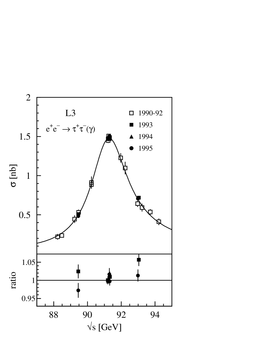
Figure 26: Same as Figure 24 for $\mathrm{e^{+}e^{-}}\rightarrow\mathrm{\tau^{+}\tau^{-}}(\mathrm{\gamma})$.

Figure 27: Same as Figure 24 for $\mathrm{e^{+}e^{-}}\rightarrow\mathrm{e^{+}e^{-}}(\mathrm{\gamma})$ inside the fiducial volume $44^{\circ}<\theta<136^{\circ}$ for acollinearity angles $\xi<25^{\circ}$ and a minimum energy of $1\ \mathrm{Ge\kern-1.00006ptV}$ of the final state fermions.

Figure 29: Same as Figure 28 for $\mathrm{e^{+}e^{-}}\rightarrow\mathrm{\tau^{+}\tau^{-}}(\mathrm{\gamma})$.

Figure 30: Same as Figure 28 for $\mathrm{e^{+}e^{-}}\rightarrow\mathrm{e^{+}e^{-}}(\mathrm{\gamma})$ in the fiducial volume $44^{\circ}<\theta<136^{\circ}$. The same cuts as for the total cross section are applied.

Figure 31: Distribution of the absolute difference of the measured cross section and forward-backward asymmetries ($1990-95$ data) and the five parameter fit result (Table 25) divided by the statistical errors of the measurements. The histogram shows the expectation for a Gaussian distribution of the measurement in the absence of systematic errors.

Figure 32: Contours in the $A_{\mathrm{FB}}^{\mathrm{0,\ell}}-R_{\mathrm{\ell}}$ plane for electrons, muons and taus obtained from a fit to total cross sections and forward-backward asymmetries. The dashed line shows the contour assuming lepton universality and the star indicates the central value. The arrows show the change in the SM prediction when varying the input parameters $\alpha_{\mathrm{s}}$ and $m_{\mathrm{H}}$ in the ranges defined in Equation 14. The uncertainty on the SM prediction due to the other parameters is small.

Figure 33: Contours in the $\bar{g}_{\mathrm{A}}$-$\bar{g}_{\mathrm{V}}$ plane for electrons, muons and taus obtained from a fit to total cross sections, forward-backward and tau polarisation asymmetries. The dashed line shows the contour assuming lepton universality and the star indicates the central value. The arrow shows the change in the SM prediction when varying $m_{\mathrm{H}}$ in the range defined in Equation 14. The uncertainty on the SM prediction due to the other parameters is small. The hollow cross indicates the SM expectation without weak radiative corrections.

Figure 34: Contour in the $j^{\mathrm{tot}}_{\mathrm{had}}$-$m_{\mathrm{Z}}$ plane obtained from the S-Matrix fit assuming lepton universality. The horizontal band shows the SM predition for $j^{\mathrm{tot}}_{\mathrm{had}}$ with its uncertainty.

Figure 35: Contour in the $m_{\mathrm{t}}$-$m_{\mathrm{W}}$ plane obtained from the SM fit to our data. The fit result is compared to our direct measurement of the W mass indicated by the hatched band and the SM expectation.

Figure 36: Contours in the $m_{\mathrm{t}}$-$m_{\mathrm{H}}$ plane obtain from the SM fit. The hatched area indicates values of the Higgs mass excluded by our direct search result [62].

Figure 37: The $\chi^{2}$ dependence of the SM fit as function of the Higgs boson mass. The shaded area indicates the mass range excluded by the direct search.

References

-
[1]
S.L. Glashow, Nucl. Phys. 22 (1961) 579;
S. Weinberg, Phys. Rev. Lett. 19 (1967) 1264;
A. Salam, “Elementary Particle Theory”, Ed. N. Svartholm, (Almqvist and Wiksell, Stockholm, 1968), 367. -
[2]
M. Veltman, Nucl. Phys. B 7 (1968) 637;
G.M. ’t Hooft, Nucl. Phys. B 35 (1971) 167;
G.M. ’t Hooft and M. Veltman, Nucl. Phys. B 44 (1972) 189; Nucl. Phys. B 50 (1972) 318. - [3] L3 Collab., B. Adeva et al., Z. Phys. C 51 (1991) 179; L3 Collab., O. Adriani et al., Physics Reports 236 (1993) 1.
- [4] L3 Collab., M. Acciarri et al., Z. Phys. C 62 (1994) 551.
- [5] ALEPH Collab., D. Decamp et al., Z. Phys. C 53 (1992) 1; D. Buskulic et al., Z. Phys. C 60 (1993) 71; Z. Phys. C 62 (1994) 539; R. Barate et al., Measurement of the Z Resonance Parameters at LEP, Preprint CERN-EP/99-104, CERN, 1999, submitted to E. Phys. J. C..
- [6] DELPHI Collab., P. Abreu et al., Nucl. Phys. B 367 (1991) 511; Nucl. Phys. B 417 (1994) 3; Nucl. Phys. B 418 (1994) 403.
- [7] OPAL Collab, G. Alexander et al., Z. Phys. C 52 (1991) 175; P.D. Acton et al., Z. Phys. C 58 (1993) 219; R. Akers et al., Z. Phys. C 61 (1994) 19.
- [8] SLD Collab., K. Abe et al., Phys. Rev. Lett. 73 (1994) 25; Phys. Rev. Lett. 78 (1997) 2075; Phys. Rev. Lett. 79 (1997) 804.
- [9] R. Assmann et al., Working Group on LEP Energy, E. Phys. J. C 6 (1999) 187.
- [10] I.C. Brock et al., Nucl. Inst. Meth. A 381 (1996) 236.
-
[11]
BHLUMI version 4.04 is used.
S. Jadach et al., Phys. Rev. D 40 (1989) 3582; Phys. Lett. B 268 (1991) 253; Comp. Phys. Comm. 70 (1992) 305;
S. Jadach, W. Placzek and B.F.L. Ward, Phys. Lett. B 353 (1995) 349;
S. Jadach et al., Phys. Lett. B 353 (1995) 362. - [12] B.F.L. Ward et al., Phys. Lett. B 450 (1999) 262.
- [13] L3 Collab., B. Adeva et al., Nucl. Inst. Meth. A 289 (1990) 35.
- [14] M. Acciarri et al., Nucl. Inst. Meth. A 351 (1994) 300.
- [15] M. Chemarin et al., Nucl. Inst. Meth. A 349 (1994) 345.
- [16] A. Adam et al., Nucl. Inst. Meth. A 383 (1996) 342.
-
[17]
JETSET version 7.4 and PYTHIA version 5.7 are used.
T. Sjöstrand, ”PHYTHIA 5.7 and JETSET 7.4 Physics and Manual”, CERN-TH 7112/93, CERN (1993), revised August 1995; T. Sjöstrand, Comp. Phys. Comm. 82 (1994) 74. -
[18]
HERWIG version 5.7 is used.
G. Marchesini and B. Webber, Nucl. Phys. B 310 (1988) 461;
G. Marchesini et al., Comp. Phys. Comm. 67 (1992) 465. -
[19]
KORALZ version 4.0 is used.
S. Jadach, B.F.L. Ward and Z. Wa̧s, Comp. Phys. Comm. 79 (1994) 503. -
[20]
BHAGENE version 3 is used.
J.H. Field, Phys. Lett. B 323 (1994) 432;
J.H. Field and T. Riemann, Comp. Phys. Comm. 94 (1996) 53. -
[21]
BHWIDE version 1.01 is used.
S. Jadach, W. Placzek and B.F.L. Ward, Phys. Lett. B 390 (1997) 298; Comp. Phys. Comm. 70 (1992) 305; Phys. Rev. D 40 (1989) 3582. -
[22]
M. Böhm, A. Denner and W. Hollik, Nucl. Phys. B 304 (1988) 687;
F.A. Berends, R. Kleiss and W. Hollik, Nucl. Phys. B 304 (1988) 712. - [23] F.A. Berends and R. Kleiss, Nucl. Phys. B 186 (1981) 22.
- [24] F.A. Berends, P.H. Daverfeldt and R. Kleiss, Nucl. Phys. B 253 (1985) 441.
-
[25]
PHOJET version 1.05 is used.
R. Engel, Z. Phys. C 66 (1995) 203;
R. Engel and J. Ranft, Phys. Rev. D 54 (1996) 4244. - [26] L3 Collab., B. Adeva et al., Z. Phys. C 55 (1992) 39.
- [27] R. Brun et al.,“GEANT 3”, CERN DD/EE/84-1 (Revised), September 1987.
- [28] H. Fesefeldt, RWTH Aachen, Preprint PITHA 85/02 (1985).
- [29] L. Arnaudon et al., Working Group on LEP Energy, Z. Phys. C 66 (1995) 45; R. Assmann et al., Working Group on LEP Energy, Z. Phys. C 66 (1995) 567.
- [30] R. Assmann and J.P. Koutschouk, “Residual Longitudinal Polarization in LEP”, Preprint CERN-SL/94-37 (AP), CERN, 1994.
- [31] L. Arnaudon et al., Working Group on LEP Energy, “The Energy Calibration of LEP in 1991“, Preprint CERN-PPE/92-125, CERN-SL/92-37(DI), CERN, 1992, also published in Proc. XXVI ICHEP, Dallas, 1992; “The Energy Calibration of LEP in 1992“, Preprint CERN-SL/93-21, CERN, 1993.
- [32] L3 Collab., M. Acciarri et al., Phys. Lett. B 370 (1996) 195.
- [33] L3 Collab., M. Acciarri et al., Phys. Lett. B 407 (1997) 361.
- [34] “The 1998 Review of Particle Physics”, C. Caso et al., E. Phys. J. C 3 (1998) 1.
- [35] A.H. Hoang, J.H. Kühn and T. Teubner, Nucl. Phys. B 455 (1995) 3.
- [36] O. Adriani et al., Nucl. Inst. Meth. A 302 (1991) 53.
-
[37]
A. Leike, T. Riemann and J. Rose, Phys. Lett. B 273 (1991) 513;
T. Riemann, Phys. Lett. B 293 (1992) 451.
See also:
A. Borelli et al., Nucl. Phys. 333 (1990) 357;
R.G. Stuart, Phys. Lett. B 272 (1991) 353. - [38] D. Bardin et al., Phys. Lett. B 206 (1988) 539.
- [39] The Working Group on LEP Energy and the LEP Collaborations: ALEPH, DELPHI, L3 and OPAL, Phys. Lett. B 307 (1993) 187.
- [40] M. Böhm et al. in “Z Physics at LEP I”, eds. G. Altarelli, R. Kleiss and C. Verzegnassi, CERN Report CERN 89-08 (1989), Vol. 1, p. 203.
- [41] F.A. Berends et al. in “Z Physics at LEP I”, eds. G. Altarelli, R. Kleiss and C. Verzegnassi, CERN Report CERN 89-08 (1989), Vol. 1, p. 89.
- [42] M. Consoli et al. in “Z Physics at LEP I”, eds. G. Altarelli, R. Kleiss and C. Verzegnassi, CERN Report CERN 89-08 (1989), Vol. 1, p. 7.
- [43] E.R. Cohen and B.N. Taylor, Rev. Mod. Phys. 59 (1987) 1121; Inst. Stand. Technol. 95 (1990) 497; W.J. Marciano and A. Sirlin, Phys. Rev. Lett. 61 (1988) 1815; T. van Ritbergen and R. Stuart, Phys. Rev. Lett. 82 (1999) 488.
- [44] G. Burgers et al. in “Z Physics at LEP I”, eds. G. Altarelli, R. Kleiss and C. Verzegnassi, CERN Report CERN 89-08 (1989), Vol. 1, p. 55.
- [45] W. Hollik, Fortschr. Phys. 38 (1990) 165.
- [46] F. Jegerlehner, in “Testing the Standard Model“ - Proceedings of the 1990 Theoretical Advanced Study Institue in Elementary Particle Physics, Boulder, Colorado, June 1990, ed. M. Cvetic and P. Langacker, World Scientific, Singapore, (1991), p. 476.
-
[47]
M. Veltman, Nucl. Phys. B 123 (1977) 89;
M.S. Chanowitz et al., Phys. Lett. B 78 (1978) 1;
M. Consoli, S. Lo Presti and L. Maiani, Nucl. Phys. B 223 (1983) 474;
J. Fleischer and F. Jegerlehner, Nucl. Phys. B 228 (1983) 1. -
[48]
ZFITTER version 6.21 is used.
D. Bardin et al., “ZFITTER v.6.21, A Semi-Analytical Program for Fermion-Pair Production in Annihilation”, Preprint DESY 99-070, hep-ph/9908433;
P. Christova, M. Jack and T. Riemann, Phys. Lett. B 456 (1999) 264;
D. Bardin et al., Phys. Lett. B 255 (1991) 290 and CERN-TH 6443/92 (May 1992); Nucl. Phys. B 351(1991) 1; Comp. Phys. Comm. 59 (1990) 303; Z. Phys. C 44 (1989) 493. -
[49]
TOPAZ0 version 4.4 is used.
G. Montagna et al., Nucl. Phys. B 401 (1993) 3; Comp. Phys. Comm. 76 (1993) 328. -
[50]
S. Jadach et al., Phys. Lett. B 257 (1991) 173;
M. Skrzypek, Acta Phys. Pol. B 23 (1992) 135;
G. Montagna et al., Phys. Lett. B 406 (1997) 243. -
[51]
S. Larin et al., Phys. Lett. B 400 (1997) 379; Phys. Lett. B 405
(1997) 327;
K.G. Chetyrkin et al., Phys. Rev. Lett. 79 (1997) 2184; Nucl. Phys. B 510 (1998) 61. - [52] A. Arbuzov, “Light Pair Corrections to Electron-Positron Annihilation at LEP/SLC”, Preprint hep-ph/9907500.
- [53] G. Degrassi et al., Phys. Lett. B 383 (1996) 219; Phys. Lett. B 394 (1997) 188; Phys. Lett. B 418 (1997) 209.
- [54] B. Kniehl, Nucl. Phys. B 347 (1990) 86.
-
[55]
A. Czarnecki and J. Kühn, Phys. Rev. Lett. 77 (1996) 3955;
R. Harlander, T. Seidensticker and M. Steinhauser, Phys. Lett. B 426 (1998) 125. - [56] W. Beenakker, F.A. Berends and S.C. van der Marck, Nucl. Phys. B 349 (1991) 323.
- [57] F. James, CERN Program Library Long Writeup D506 MINUIT, CERN, 1993.
- [58] “Reports of the Working Group on Precision Calculations for the Resonance”, eds. D. Bardin, W. Hollik and G. Passarino, CERN Report CERN 95-03 (1995).
- [59] D. Bardin, M. Grünewald and G. Passarino, “Precision Calculation Project Report, Preprint hep-ph/9902452.
- [60] W. Beenakker and G. Passarino, Phys. Lett. B 425 (1997) 199.
- [61] CDF Collab., F. Abe et al., Phys. Rev. Lett. 74 (1995) 2626; Phys. Rev. Lett. D 80 (1998) 2767; Phys. Rev. Lett. D 80 (1998) 2779; Preprint FERMILAB PUB-98/319-E, submitted to Phys. Rev. Lett.; Phys. Rev. Lett. D 82 (1999) 271, Erratum, ibid. D 82 (1999) 2808; DØ Collab., S. Abachi et al., Phys. Rev. Lett. 74 (1995) 2632; B. Abott et al., Phys. Rev. Lett. D 80 (1998) 2063; Phys. Rev. D 58 052001 (1998); Phys. Rev. D 60 052001 (1999). We use the average top mass as given in Reference [34].
- [62] L3 Collab., M. Acciarri et al., Phys. Lett. B 461 (1999) 376.
-
[63]
M. Veltman, Acta Phys. Polon. B 8 (1977) 475;
B.W. Lee, C. Quigg and H.B. Thacker, Phys. Rev. D 16 (1977) 1519. - [64] S. Eidelman and F. Jegerlehner, Z. Phys. C 67 (1995) 585.
- [65] L3 Collab., M. Acciarri et al., Phys. Lett. B 431 (1998) 387.
- [66] Particle Data Group, “Review of Particle Properties“, Phys. Rev. D 54 (1996) 1.
- [67] L3 Collab., M. Acciarri et al., Phys. Lett. B 429 (1998) 387.
- [68] CHARM II Collab., P. Vilain et al., Phys. Lett. B 335 (1994) 246.
- [69] L3 Collab., M. Acciarri et al., Phys. Lett. B 448 (1999) 152.
- [70] L3 Collab., M. Acciarri et al., Phys. Lett. B 439 (1998) 225.
-
[71]
SMATASY version 6.21 is used.
S. Kirsch and T. Riemann, Comp. Phys. Comm. 88 (1995) 89. - [72] L3 Collab., O. Adriani et al., Phys. Lett. B 315 (1993) 494.
- [73] L3 Collab., M. Acciarri et al., Measurement of and at LEP Using Double-Tag Methods, Preprint CERN-EP/99-121, CERN, 1999, accepted by E. Phys. J. C.
- [74] L3 Collab., M. Acciarri et al., Phys. Lett. B 444 (1998) 569.
- [75] L3 Collab., M. Acciarri et al., Phys. Lett. B 398 (1997) 223.
- [76] L3 Collab., M. Acciarri et al., Phys. Lett. B 413 (1997) 176.
- [77] L3 Collab., M. Acciarri et al., Phys. Lett. B 454 (1999) 386.