ICANOE
Imaging and Calorimetric Neutrino Oscillation Experiment

Abstract

The main scientific goal of the ICANOE detectoricanoe is the one of elucidating in a comprehensive way the pattern of neutrino masses and mixings, following the SuperKamiokande results and the observed solar neutrinos deficit. To achieve these goals, the experimental method is based upon the complementary and simultaneous detection of CERN beam (CNGS) and cosmic ray (CR) events. For the currently allowed values of the SuperKamiokande results, both CNGS and cosmic ray data will give independent measurements and provide a precise determination of the oscillation parameters. Since one will observe and unambiguously identify ${\nu_{e}}$, ${\nu_{\mu}}$ and ${\nu_{\tau}}$ components, the full (3 x 3) mixing matrix will be explored.

1 Introduction

The reference mass for underground detectors is now set by the operating SuperKamiokandesuperk detector, which is of the order of 30 ktons. However the rather coarse nature of the Cherenkov ring detection is capable to reconstruct only part of the features of the events.

New generation underground experiments are now facing new challenges, for which novel and more powerful technologies are required, with respect to the existing detectors:

1. The long baseline accelerator neutrino oscillation experiments require, with respect to existing short baseline detectors (like NOMADnomad and CHORUSchorus ), a large increase of the detector fiducial mass (about 3 ton in NOMAD), in order to cope with the flux attenuation due to the distance. In order to perform a comprehensive program on neutrino oscillations the fiducial mass of the detector must be increased to several ktons. Moreover, the detector must be able to tag efficiently the interaction of ${\nu_{e}}$’s and ${\nu_{\tau}}$’s out of the bulk of ${\nu_{\mu}}$ events. This requires a detailed event reconstruction that can be achieved only by means of a high granularity detector.

2. Likewise, the comprehensive investigation of atmospheric neutrinos events, in order to reach the level of at least one thousand events/year, also requires a fiducial mass of several ktons. The capability to observe all separate processes, electron, muon and tau neutrino charged currents (CC) and all neutral currents (NC) without detector biases and down to kinematical threshold is highly desirable.

3. Nucleon decay: because of the already very high limit on the nucleon lifetime ($\geq 10^{32}$ years in most of the decay channels), a modern proton decay detector should have an adequately large sensitive mass.

Event imaging should be provided by a modern bubble chamber-like technology since (1) it has to be able to provide high resolution, unbiased, three dimensional images of ionising events; (2) it has to provide an accurate measurement of the basic kinematical properties of the particles of the event, including particle identification. (3) it has to accomplish simultaneously the two basic functions of target and detector.

In the ICANOE design a fully sensitive, bubble chamber-like detector will permit discovery limits at the few events level and a much more powerful background rejection. A detector of this kind, already at the level of a few ktons of mass will be fully competitive with the potentialities of SuperKamiokande and in several domains will permit to extend much further the investigations.

The ICANOE detector fruitfully merges the superior imaging quality of the ICARUS technologyicaruswww with the high resolution full calorimetric containment of NOEnoewww , suitably upgraded to provide also magnetic analysis of muons. It has a modular structure of independent supermodules and is expandable by the addition of such supermodules, each consisting of a low density 1.9 kton liquid target and of a high density 0.8 kton active solid target.

The superior quality of the event vertex inspection and reconstruction of the liquid Argon is ideally complemented by the addition of the external module capable of magnetic analysis of the muons escaping the LAr chamber. Bubble chambers have in fact often been very similarly complemented in the past by external identifiers. An iron muon tracking spectrometer would fulfill this job, but it would also introduce in between adjacent liquid argon volumes a blind region incapable of giving information on the energy and on the nature of the escaping particles. A sensitive magnetized calorimeter appears therefore as an ideal containment module to be interleaved between adjacent liquid Argon volumes.

2 Outline of the ICANOE detector

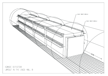
Figure 1: Perspective view of the baseline detector with 4 supermodules.

The ICANOE layout (Figure 1) is similar to that of a “classical” neutrino detector, segmented into almost independent supermodules. The layout of the apparatus can be summarized as follows:

• the liquid target, with extremely high resolution, dedicated to tracking, $dE/dx$ measurements, full e.m. calorimetry and hadronic calorimetry, where electrons and photons are identified and measured with extremely good precision and $\pi/\mu$, $K$ and $p$ separation is possible at low momenta;

• the solid target, with good e.m. and hadronic resolution, dedicated to calorimetry of the jet and a magnetic field for measurement of the muon features (sign and momentum);

• The supermodule, obtained joining a liquid and solid module, which constitutes the basic module of an expandable apparatus. A supermodule behaves as a complete building block, capable of identifying and measuring electrons, photons, muons and hadrons produced in the events. The solid, high density sector reduces the transverse and longitudinal size of hadron shower, confining the event (apart from the muon) within the supermodule.

The ICANOE SuperModule is, according to the present design, composed by a liquid Argon module, with 18.0$\times$ (11.3)² m³ of external dimensions and 1.4 kton (1.9 kton) of active (total) mass, and a magnetized calorimeter module, with 2.6$\times$ 9² m³ of external dimensions and 0.8 kton of mass. The depth consists of 2 m for the calorimetric unit, corresponding to $7.4\ \lambda_{int}$ and $59\ X_{0}$ and $0.6$ m for the tracking units (the interleaved planes of tracking chambers).

At this stage, four SuperModules with a total length of the experiment of $82.5$ m and a total active mass of 9.3 kton fully instrumented are being considered for the baseline option.

3 Physics goals

ICANOE is an underground detector capable to achieve the full reconstruction of neutrino (and antineutrino) events of any flavor, and with an energy ranging from the tens of MeV to the tens of GeV, for the relevant physics analyses. No other combinations can provide such a rich spectrum of physical observations, including the systematic, on-line monitoring of the CNGS $\nu$-beam at the LNGS site. The unique lepton capabilities of ICANOE are really fundamental in tagging the neutrino flavor. In general, the oscillation pattern of the neutrinos may be complicated and involve a combination of ${\nu_{\mu}}\rightarrow{\nu_{\tau}}$, ${\nu_{\mu}}\rightarrow{\nu_{e}}$ and ${\nu_{\mu}}\rightarrow\nu_{sterile}$ transitions. In order to fully sort out the mixing matrix, unambiguous neutrino flavor identification is mandatory to distinguish $\tau$’s from $\nu_{\tau}$’s and electrons from $\nu_{e}$’s interactions. In other words, we stress the importance of constraining the oscillation scenarios by coupling appearance in several different channels and disappearance signatures.

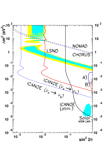
Figure 2: Overview of the status of the neutrino oscillations searches, displayed assuming two neutrino mixing schemes in the $(\sin^{2}2\theta,\Delta m^{2})$ plane. The 90%C.L. allowed regions obtained from the Kamiokande (resp. Superkamiokande) FC and PC samples are shown as A) (resp. B)). The 90% (resp. 99%C.L.) regions consistent with the LSND excess are shown as dark (resp. light) shaded areas in the upper region of the plane. The shaded area in the region $\Delta m^{2}\approx 10^{-5}\ \rm eV^{2}$ represents the large angle MSW solution of the solar neutrino deficit. CHORUS and NOMAD 90%C.L. limits on ${\nu_{\mu}}\rightarrow{\nu_{\tau}}$ oscillations are visible in the upper $\Delta m^{2}$ region. The ICANOE sensitivities at 90%C.L. are indicated by three curves: the limit by direct observation of the atmospheric neutrinos (“ICANOE atm”); the direct tau appearance search at the CNGS (“ICANOE ${\nu_{\mu}}\rightarrow{\nu_{\tau}}$”); the direct electron appearance search at the CNGS (“ICANOE ${\nu_{\mu}}\rightarrow{\nu_{e}}$”).

The sensitivity in the classic $(\sin^{2}2\theta,\Delta m^{2})$ plot is evidenced in Figure 2, for a data taking time of 4 years, with $4.5\times 10^{19}$ pot at each year. We remark:

1. The recent results on atmospheric neutrinos (“A” and “B” of Figure 2) can be thoroughly explored by appearance and disappearance experiments. For the current central value, both CNGS and cosmic ray data will give independent and complementary measurements and they will provide a precise $(\sin^{2}2\theta,\Delta m^{2})$ determination.

2. In the mass range of LSND, the sensitivity is sufficient in order to solve definitely the puzzle.

3. At high masses of cosmological relevance for $\Delta m^{2}<\approx 10\rm\ eV^{2}$, the sensitivity to ${\nu_{\mu}}\rightarrow{\nu_{\tau}}$ oscillations is better or equal to the one of CHORUS and NOMAD.

4. In the atmospheric neutrino events, one can reach a level of sensitivity sufficient to detect also the effect until now observed in solar neutrinos. This purely terrestrial detection of the LMA solar neutrino solution is performed using neutrino in the GeV range, much higher than the one of solar neutrinos.

Since we can observe and unambiguously identify both ${\nu_{e}}$ and ${\nu_{\tau}}$ components, the full (3 x 3) mixing matrix can be explored. By itself, this is one of the main justifications for the choice of the detector’s mass.

In the cosmic ray channel, all specific modes (electron, muon, NC) are equally well observed without detector biases and down to kinematical threshold. The CR-spectrum being rather poorly known, a confirmation of the SuperKamiokande result requires detecting both (1) the modulation in the muon channel and (2) the lack of effect of the electron channel. The consistency of the simultaneous observation of the $L/E$ phenomenon in as many modes as they are available is a powerful tool in separating genuine flavour oscillations from exotic scenarios.

In some favourable conditions, the direct appearance of the oscillated tau neutrino may be directly identified in the upgoing events, since even a few events will be highly significant.

While in atmospheric neutrinos, the knowledge of the sign of the muon is of little relevance, in the case of the CNGS is a powerful tool to verify the neutrino nature after oscillation path, excluding for instance oscillation channels into anti-neutrinos.

For a discussion on the nucleon decay searches, see Ref. NNNnucdec .

4 Physics at the CNGS

The design and performance of the CERN neutrino beam to Gran Sasso - the CNGS facility - are described in a conceptual technical design report NGSreport . The CNGS beam performance for the new reference beam are summarized in Table 1. The rms radius of the $\nu_{\mu}$ CC event distribution is about 1.37 km at Gran Sasso. The expected numbers of detectable $\nu_{\tau}$ for $\sin^{2}2\theta$ = 1 and a few typical values of $\Delta m^{2}$ are shown in Table 2.

Energy region $E_{\nu_{\mu}}$ [GeV]	1 - 30	1 - 100
$\nu_{\mu}$ [m-2/pot]	7.1 $\times$ 10-9	7.45 $\times$ 10-9
$\nu_{\mu}$ CC events/pot/kt	4.70 $\times$ 10-17	5.44 $\times$ 10-17
$\mbox{$\left\langle E\right\rangle$}_{\nu_{\mu}\,fluence}$ [GeV]		17
fraction of other events:
$\nu_{e}$/$\nu_{\mu}$	0.8 %
$\overline{\nu}_{\mu}$/$\nu_{\mu}$	2.0 %
$\overline{\nu}_{e}$/$\nu_{\mu}$	0.05 %

Table 1: Predicted performance of the new CNGS reference beam for an isoscalar target. The statistical accuracy of the Monte-Carlo simulations is 1 % for the $\nu_{\mu}$ component of the beam, somewhat larger for the other neutrino species.

Energy region $E_{\nu_{\tau}}$ [GeV]	1 - 30	1 - 100
$\Delta m^{2}$ = 1 $\times$ 10-3 eV2	2.34	2.48
$\Delta m^{2}$ = 3 $\times$ 10-3 eV2	20.7	21.4
$\Delta m^{2}$ = 5 $\times$ 10-3 eV2	55.9	57.7
$\Delta m^{2}$ = 1 $\times$ 10-2 eV2	195	202

Table 2: Expected number of $\nu_{\tau}$ CC events at Gran Sasso per kton per year for an isoscalar target. Results of simulations for different values of $\Delta m^{2}$ and for $sin^{2}(2\theta)$ = 1 are given for 4.5 $\times$ 10¹⁹ pot/year. These event numbers do not take detector efficiencies into account.

Events will occur in the whole ICANOE detector. As reference, we assume an exposure of $20\ \rm kton\times year$ for the liquid argon. This corresponds to four years running of the CNGS beam in shared mode. For the events occuring in the solid detector, given the smaller mass, the reference exposure is $10\ \rm kton\times year$. The last three meters of the liquid target are defined as a transition region, since beam events occuring in this region are most likely to deposit energy in both targets. Table 3 shows the computed total event rates for each neutrino species present in the beam for the liquid, solid and in the transition region. Table 3 also shows, for three different values of $\Delta m^{2}$, the $\nu_{\tau}$ CC rates expected in case oscillations take place.

Process	liquid target	transition	solid
$\nu_{\mu}$ CC	54300	10200	27150
$\bar{\nu}_{\mu}$ CC	1090	200	545
$\nu_{e}$ CC	437	80	219
$\bar{\nu}_{e}$ CC	29	5	15
$\nu$ NC	17750	3330	8875
$\bar{\nu}$ NC	410	77	205
${\nu_{\tau}}$ CC, $\Delta m^{2}$ (eV2)
$1\times 10^{-3}$	52	10	26
$2\times 10^{-3}$	208	40	104
$3.5\times 10^{-3}$	620	115	310
$5\times 10^{-3}$	1250	235	625
$7.5\times 10^{-3}$	2850	535	1425
$1\times 10^{-2}$	4330	810	2165

Table 3: Expected event rates for an exposure of 20 kton$\times$ year for the liquid target and 10 kton$\times$ year for the solid target. All the rates include nuclear corrections and are computed for the proper target composition. For standard processes, no oscillations is assumed. For $\nu_{\tau}$ CC, we take two neutrino $\nu_{\mu}\rightarrow\nu_{\tau}$ with $\sin^{2}2\theta=1$.

4.1 Event kinematics and tau identification

Kinematical identification of the $\tau$ decay, which follows the ${\nu_{\tau}}$ CC interaction requires excellent detector performance: good calorimetric features together with tracking and event topology reconstruction capabilities. The background from standard processes are, depending on the decay mode of the tau lepton considered, the ${\nu_{e}}$ CC events and/or the ${\nu_{\mu}}$ CC and $\nu$ NC events.

In order to separate separate ${\nu_{\tau}}$ events from the background, two basic criteria, already adopted by the short baseline NOMAD experiment, can be used:

• an unbalanced total transverse momentum due to neutrinos produced in the $\tau$ decay,

• a kinematical isolation of hadronic prongs and missing momentum in the transverse plane.

In addition, given the baseline $L$ between CERN and GranSasso, for the lower $\Delta m^{2}$ values of the allowed region indicated by the atmospheric neutrino results, we expect most of the oscillation to occur at low energy. In this case, a criteria on the visible energy is also very important to suppress backgrounds.

In order to apply the most efficient kinematic selection, it is mandatory to reconstruct with the best possible resolution the energy and the angle of the hadronic jet, with a particular attention to the tails of the distributions. Therefore, the energy flow algorithm should be designed with care taking into account the needs of the tau search analyses.

A specially developed energy flow algorithm has been tested on a sample of fully simulated ${\nu_{e}}\ \rm CC$ events, in order to estimate the resolution of the kinematical reconstruction on realistic events. It yields an average missing $P_{T}$ of $450\ \rm MeV/c$. This value improves to an average of $410\ \rm MeV/c$ when the primary vertex is required to lie within a fiducial volume of transverse dimensions $7.8\times 7.8m^{2}$.

We used the neutrino data collected in the NOMAD detector to probe the reliability of the physics simulation. $\nu_{\mu}$ CC events have been fully simulated and reconstructed using NOMAD official packages. We found that the kinematics in the transverse plane are well reproduced by the Monte-Carlo model. This is clearly not the case when nuclear corrections are neglected.

Cuts	$\nu_{\tau}$ Eff.	$\nu_{e}$	${\bar{\nu}}_{e}$	$\nu_{\tau}$ CC	$\nu_{\tau}$ CC	$\nu_{\tau}$ CC
	($\%$)	CC	CC	$\Delta m^{2}=$	$\Delta m^{2}=$	$\Delta m^{2}=$
				$10^{-3}$ eV2	$3.5\times 10^{-3}$ eV2	$10^{-2}$ eV2
Initial	100	437	29	9.3	111	779
Fiducial volume	88	383	25	8.2	97	686
One candidate with
momentum $>1$ GeV	72	365	25	6.7	80	561
$E_{vis}<18$ GeV	67	64	5	6.2	75	522
$P_{T}^{e}<0.9$ GeV	54	31	3	5.0	60	421
$P_{T}^{lep}>0.3$ GeV	51	29	2	4.7	56	397
$P_{T}^{miss}>0.6$ GeV	33	4	0.4	3.1	37	257

Table 4: Rejection of the ${\nu_{e}}$ CC background in the $\tau\rightarrow e$ analysis. Figures are normalized to an exposure of 20 kton $\times$ year.

4.2 ${\nu_{\mu}}\rightarrow{\nu_{\tau}}$ appearance searches

The channel of tau decaying into an electron plus two neutrinos provides the best sample for ${\nu_{\tau}}$ appearance studies due to the low background level. The intrinsic ${\nu_{e}}$, $\bar{\nu_{e}}$ contaminations of the beam amount to $\approx 470$ events for an exposure of $20\ \rm kton\times year$.

The comparison of this figure with the expected number of ${\nu_{\tau}}$ CC events decaying into electrons shows that the search of $\tau\rightarrow e$ at the CNGS will have to be optimized a posteriori. Indeed the ${\nu_{\tau}}$ rate has a strong dependence on the exact value of the $\Delta m^{2}$ in the parameter region suggested by the Super-Kamiokande data, and the $\Delta m^{2}$ value is not well constrained by the atmospheric neutrino experiments.

For “large” values of $\Delta m^{2}$, i.e. $\Delta m^{2}>5\times 10^{-3}$, the rate of tau is spectacular and exceeds the number of intrinsic beam ${\nu_{e}}$, $\bar{\nu_{e}}$ CC events, i.e. $S/B>1$ even prior to any kinematical cuts. So the kinematical cuts can be very mild. An excess will be striking.

For our “best” value taken from atmospheric neutrino results, i.e. $\Delta m^{2}=3.5\times 10^{-3}\ \rm eV^{2}$, the number of ${\nu_{\tau}}~{}CC$ with $\tau\rightarrow e$ is about 110, or about a signal over background ratio of $110/470\simeq 1/4$. Here with modest kinematical cuts, we can extract statistically significant signals, as shown in the following sections.

The most difficult region lies below $\Delta m^{2}\approx 1.5\times 10^{-3}\ \rm eV^{2}$, for which, kinematical cuts are tuned to suppress backgrounds by a factor more than 200 while keeping about half of the signal events.

Cuts	$\nu_{\mu}$ NC
Initial	17750
Fiducial volume	15550
	Dalitz	$\gamma$ conv.	$\pi\rightarrow e$	$\pi^{\pm}/\pi^{0}$
One candidate	275	4262	6.5	25
$P_{e}>1$ GeV	79	1361	6.3	16
$E_{vis}<18$ GeV	49	835	3.2	11
$P_{T}^{e}<0.9$ GeV	46	794	1.8	9
$P_{T}^{lep}>0.3$ GeV	24	429	1.7	8
$P_{T}^{miss}>0.6$ GeV	19	350	1.3	7
Imaging and $dE/dx$	$<1$	$<1$	$<1$	$<1$

Table 5: $\nu_{\mu}$ NC background to the $\tau\rightarrow e$ analysis. Results are normalized to an exposure of 20 kton $\times$ year. We illustrate background reduction by means of kinematical criteria only. Imaging and $dE/dx$ measurements reduce the NC background to a negligible level.

In the following paragraphs, we discuss background sources and their suppression.

${\nu_{e}}~{}CC$ rejection: The main background from genuine leading electrons comes from the CC interactions of the $\nu_{e}$ and $\bar{\nu}_{e}$ components of the beam. In Table 4 we summarize the list of sequential cuts applied to reduce the $\nu_{e}$ and $\bar{\nu}_{e}$ CC backgrounds and the expected number of signal events for three different $\Delta m^{2}$ values. The most sensitive analysis predicts, for a 20 kton $\times$ year exposure, a total background of 4.4 events for a total $\tau$ selection efficiency of 33$\%$.

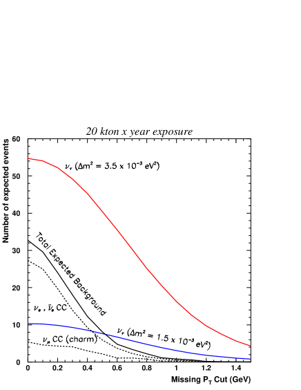
Figure 3: Number of $\nu_{e},\ \bar{\nu}_{e}$ background and tau events expected for a 20 kton $\times$ year exposure as a function of the missing transverse momentum.

$\nu~{}NC$ rejection: Neutral current events contribute to the background from four sources: (1) electrons from Dalitz decays, (2) early photon conversions, (3) interacting charged pions and (4) $\pi^{\pm}/\pi^{0}$ overlap. Table 5 summarizes the rejection power of kinematics criteria for the four sources that contribute to $\nu~{}NC$ background. The requirement on the electron candidate energy $E_{e}>1\ \rm GeV$ suppresses about one third of the Dalitz, pion overlap and $\pi^{0}$ conversions induced backgrounds, since electrons in the jet are soft.

The ultimate discrimination of these backgrounds relies primarily on the imaging capabilities and on $dE/dx$ measurements. The combination of $dE/dx$ information together with kinematics criteria is sufficient to reduce $\nu~{}NC$ background to a negligible level.

${\nu_{\mu}}~{}CC$ rejection: Charged current events can contribute to the background in a similar way as the neutral current events described above when the leading muon escapes detection. In case the muon is not identified, the event will appear in first instance as a neutral current event. The source of electrons which can induce backgrounds are then similar to those discussed previously and are reduced to a negligible level for reasons already discussed. A more important source of background specific to charged current interactions comes from the decays of charmed mesons. At the CNGS energies $\sigma(\nu_{\mu}N\rightarrow\mu\ c\ X)/\sigma(\nu_{\mu}N\rightarrow\mu X)\approx 4\%$, therefore for a total exposure of 20 kton $\times$ year we expect to collect about 200 events where a charmed meson decays into a positron and a neutrino. These events resemble kinematically the real $\nu_{\tau}$ events, since they have a neutrino in the final state and possess a softer energy spectrum and a genuine sizeable missing transverse momentum. After all cuts, the expected number of charm induced background events $n^{b}_{CC\ (charm)}$ for a total exposure of 20 kton $\times$ year is at the level of 1 event.

$\Delta m^{2}$ (eV2)	$\nu_{\tau}$ CC	$\nu_{e},\ {\bar{\nu}}_{e}$ CC	$\nu_{\mu},\ {\bar{\nu}}_{\mu}$ CC	$\nu_{\mu}$ NC
$1\times 10^{-3}$	3
$2\times 10^{-3}$	12
$3\times 10^{-3}$	26
$3.5\times 10^{-3}$	35	4.1	1.0	$<1$
$5\times 10^{-3}$	71
$7\times 10^{-3}$	121
$1\times 10^{-2}$	248

Table 6: $\tau\rightarrow e$ analysis summary. For a total exposure of 20 $\times$ year we show the expected number of $\tau$ events for different $\Delta m^{2}$ values. The last three columns show the expected background.

4.3 Combined ${\nu_{\mu}}\rightarrow{\nu_{\tau}}$ sensitivity

Table 6 summarizes the expectations for the $\tau\rightarrow e$ analysis once kinematics criteria and muon vetoes have been applied to every potential background source. In conclusion, we obtain for a 20 kton $\times$ year exposure, that the overall electron selection efficiency is 32$\%$ for an expected number of about five background events. The expected number of fully identified tau events at the central $\Delta m^{2}$ value of $3.5\times 10^{-3}$ eV² is 35.

We show in Figure 3 as a function of the cut on the missing transverse momentum, the number of expected background and tau events for two different $\Delta m^{2}$ values. We see that even for a value as low as $1.5\times 10^{-3}$ eV², a $P_{T}^{miss}$ cut above 0.6 GeV gives a $S/B$ ratio in excess of 1.

Finally it is crucial to study the exposures needed to obtain a statistically significant $\tau$ appearance for different neutrino oscillation scenarios. We see in Figure 4 that for $\Delta m^{2}=3.5$ eV², few months of data taking will suffice to claim a 3$\sigma$ effect. However for $\Delta m^{2}$ values of about $10^{-3}$ eV², exposures above 20 kton $\times$ year are needed to obtain an effect in excess of 2$\sigma$. We conclude that after four years of running of CNGS in shared mode or after one year of running in dedicated mode, the ICANOE detector will observe a statistically significant $\nu_{\mu}\rightarrow\nu_{\tau}$ oscillation signal for most of the $\Delta m^{2}$ values presently favored by atmospheric neutrino data.

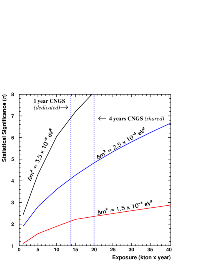
Figure 4: $\tau$ appearance statistical significance for different $\Delta m^{2}$ values as a function of the exposure. The arrows indicate the statistical significance achieved for one year of dedicated run of the CNGS and four years of CNGS running in shared mode.

4.4 ${\nu_{\mu}}\rightarrow{\nu_{e}}$ oscillation search

The unambiguous detection and identification of $\nu_{e}$ CC events endows ICANOE with the ability of performing also a $\nu_{\mu}\rightarrow\nu_{e}$ oscillation search. In this case, the oscillation reveals itself as an excess on the number of expected events having a leading identified electron. Given the expected rates for a 20 kton $\times$ year exposure, the statistical error is about 4$\%$. Therefore the sensitivity to $\nu_{\mu}\rightarrow\nu_{e}$ oscillations is dominated by the systematic error on the beam knowledge.

Figure 5 shows the 90$\%$ C.L. contours in case no oscillations are observed assuming overall systematic errors of 5$\%$ and 10$\%$. We observe that nearly the whole region favored by the LSND claim is comfortably covered. The excluded values are $\sin^{2}2\theta>2\times 10^{-3}$ at high $\Delta m^{2}$ and $\Delta m^{2}>4\times 10^{-4}$ eV² for maximal mixing.

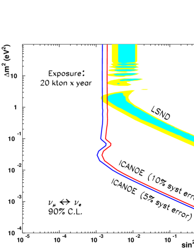
Figure 5: ICANOE 90$\%$ C.L. exclusion region in case no $\nu_{\mu}\rightarrow\nu_{e}$ are experimentally observed.

5 Atmospheric neutrinos

The physics goals of the new atmospheric neutrino measurements are to firmly establish the evidence of neutrino oscillations with a different experimental technique, possibly free of systematic biases, measure the oscillation parameters and clarify the nature of the oscillation mechanism. ICANOE will provide, in addition to comfortable statistics, an observation of atmospheric neutrinos of a very high quality. Unlike measurements obtained up to now in Water Cherenkov detectors, which are in practice limited to the analysis of “single-ring” events, complicated final states with multi-pion products, occurring mostly at energies higher than a few GeV, will be completely analyzed and reconstructed in ICANOE. This will be a significant improvement with respect to previous observations.

We have considered the following three methods:

• ${\nu_{\mu}}$ disappearance: detection of the oscillation pattern in the $L/E$ distribution, where $L$ is the neutrino pathlength and $E$ its energy;

• $\nu_{\tau}$ appearance : comparison of the NC/CC with expectation;

• direct $\nu_{\tau}$ appearance : comparison of upward and downward rates of “tau-like” events.

together with the well established ones:

• the double ratio, $({\nu_{\mu}}/{\nu_{e}})_{obs}/({\nu_{\mu}}/{\nu_{e}})_{MC})$;

• up/down asymmetry;

The tau appearance measurements can shed light on the nature of the oscillation mechanism, by discriminating between the hypothesis of oscillations into a sterile or a tau neutrino. The $\nu_{\tau}$ appearance method is based on $\nu_{\tau}$ CC interactions with $\nu_{\tau}$ decaying into hadrons, hence to “neutral-current-like” events of high energy. An excess of “NC-like” events from the bottom will indicate the presence of oscillation to the $\nu_{\tau}$ flavour. A kinematical analysis of the final state particles in the event can be used to further improve the statistical significance of the excess. Such a feature can only be obtained in a detector with the resolution of the ICANOE liquid target, in which all final state particles can be identified and precisely measured. The kinematical method would allow the evidence for “tau-like” events in the atmospheric neutrino beam.

Both the $\nu_{\mu}$ disappearance and the direct $\nu_{\tau}$ appearance methods are weakly depending on the predictions of neutrino event rates, since they rely on the comparison of rates induced by a downward going and upward going neutrinos.

The $NC/CC$ method, already investigated by SuperKamiokande, can be significantly improved compared to this latter measurement. In ICANOE, imaging in the liquid target provides a clean bias free identification of neutral-current, independent on the hadronic final state, since the identification is based on the absence of an electron or a muon in the final state.

In the following sections, we will study our results for three different exposures: 5 kton$\times$year corresponding to 1 year of operation, 20 kton$\times$year for 4 years and an ultimate exposure of 50 kton$\times$year or 10 years of operation.

The computed rates for the different neutrino processes (in events/kton/year) and their mean energies are quoted in Table 7, using the FLUKA-3D atmospheric neutrino fluxes1d3d .

Process	elastic	single-$\pi$	inelastic	Total	$<$E$>$
					(GeV)
$\nu_{\mu}\rm\ CC$	66.7	15.9	24.4	107.0	2.36
$\bar{\nu}_{\mu}\rm\ CC$	12.2	5.3	9.8	27.2	3.34
$\nu_{e}\rm\ CC$	39.4	8.4	12.1	59.9	1.60
$\bar{\nu}_{e}\rm\ CC$	5.4	2.1	4.2	11.7	2.36
$\nu\rm\ NC$	42.9	8.6	13.2	64.8	1.94
$\bar{\nu}\rm\ NC$	21.1	3.5	5.0	29.6	2.00

Table 7: Expected atmospheric neutrino rates per kton$\times$year on Argon in case of no oscillations. The figures have been computed with FLUKA 3D atmospheric neutrino flux with geomagnetic cutoffs and include all nuclear effects. All NC events are included, even though only a fraction of quasi-elastic ones will end up in an observable final state.

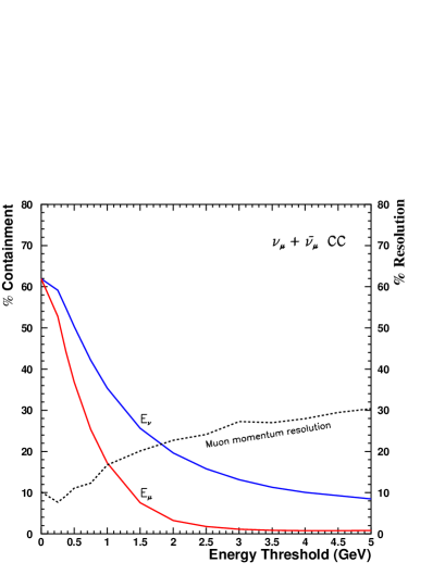
Figure 6: Integral distributions showing the containment for $\nu_{\mu}$ CC as a function of the neutrino energy and the leading muon momentum (solid lines). Differential distribution showing the muon momentum resolution as a function of muon momentum (dashed line), including both contained and partially contained events.

5.1 Event containment and muon measurement

The muon measurement is crucial to most atmospheric neutrino analyses. In ICANOE, we achieve the required performances using the multiple scattering measurement rather than resorting to a high–density, coarser resolution detector. Keeping a low density detector, high granularity detector imaging allows in addition the identification and measurement of electrons and individual hadrons in the event.

“Fully contained events” are those for which the visible products of the neutrino interaction are completely contained within the detector volume. “Partially contained events” are ${\nu_{\mu}}\rm\ CC$ events for which the muon exits the detector volume (only muons are penetrating enough).

Figure 6 shows containment of charged current events for different incoming neutrino energies or muon momentum thresholds. Clearly, because of the average energy loss of the muon in argon (about $210\rm\ MeV/m$ for a m.i.p.), muons produced in neutrino events are often energetic enough to escape from the subdetector volume.

It should first be noted that for contained events the muon energy resolution is $4\%$ from $dE/dx$ measurements. For escaping muons, the high granularity of the imaging allows to collect a very precise determination of the track trajectory. Therefore the multiple scattering method can be effectively used to estimate the momentum of the escaping muons. This method requires in practice tracks in excess of 1 meter and works extremely well in the relevant energy range of atmospheric neutrino events (typically below 10 GeV).

The average muon momentum resolution as a function of the energy threshold is shown in Figure 6. This resolution has been computed using the range measurement for contained muons and multiple scattering method for the escaping ones. For energies below 1 GeV, the average muon momentum resolution is about 10%. It increases slowly as a function of the muon momentum and reaches about 30% at 5 GeV.

5.2 Incoming neutrino angular resolution

The reconstruction of the zenith angle of the incoming $\nu$ is of great importance in the search of oscillations in atmospheric neutrinos. ICANOE allows for a good reconstruction of the incoming neutrino variables (i.e. incidence angle, energy) by using the information coming from all particles produced in the final state. Figure 7 shows the distribution of the difference between the real and reconstructed neutrino angle for events with $E_{\nu}>1$ GeV. The improvement on the angular resolution is visible. The RMS of the distribution improves from $\sim 16$ to $\sim 8$ degrees after the inclusion of the hadronic jet in the reconstruction.

Figure 7: Zenith angle resolution. The top plot shows the resolution obtained by reconstructing the incoming neutrino direction using all particles momenta, the bottom plot shows the resolution obtained using only leading lepton momentum.

5.3 The flavor ratio and up/down asymmetry

Given the clean event reconstruction of ICANOE, the ratio $R$ of “muon-like” to “electron-like” events can be determined free of experimental systematic errors. In fact, the expected purity of the samples is above 99%. In particular, the contamination from $\pi^{0}$ in the “electron-like” sample is expected to be completely negligible. The measurement accuracy will be dominated by the statistical uncertainty and by the theoretical systematic error on the double ratio.

In order to estimate statistical sensitivities, we show in Table 8 the values and statistical errors of $R$ for different exposures, assuming an oscillation $\nu_{\mu}\rightarrow\nu_{x\neq\mu}$, with parameters $\sin^{2}2\theta=1$ and $\Delta m^{2}=3.5\times 10^{-3}\rm\ eV^{2}$. The table lists the expected results when using all events or only fully contained events which turn out to be quite similar.

Clearly, after an exposure corresponding to about four years of running of ICANOE, the statistical error reaches a level below 5%. We expect that further theoretical improvements should reduce the systematic error to a level matched to statistical precision achievable in ICANOE.

Exposure (kton$\times$year)	$R$
	all events	contained
5	$0.696\pm 0.067$	$0.674\pm 0.074$
20	$0.696\pm 0.033$	$0.674\pm 0.037$
50	$0.696\pm 0.021$	$0.674\pm 0.023$

Table 8: $R$ as a function of the exposure assuming maximal mixing and $\Delta m^{2}=3.5\times 10^{-3}$ eV². In left column: results obtained by using all events; right column: results obtained by using only fully contained events. Quoted errors are of statistical nature.

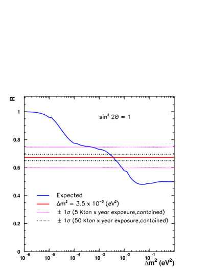
Figure 8: Expected $R$ value as a function of $\Delta m^{2}$. Assuming a true $\Delta m^{2}$ value of $3.5\times 10^{-3}$ eV², the $68\%$ confidence intervals are given for 5 and 50 kton$\times$year.

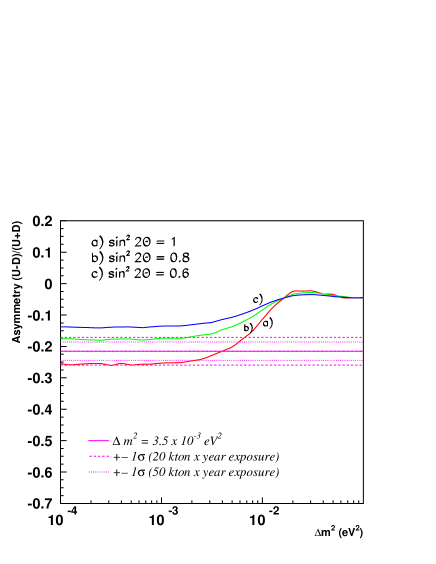
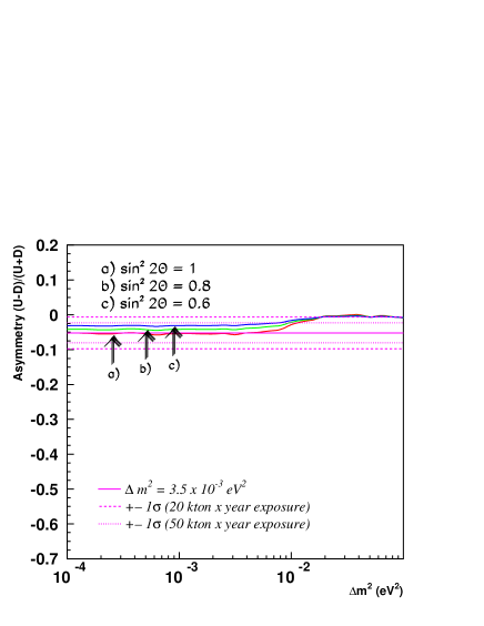
Figure 9: Expected Up-Down asymmetry for $\sin^{2}(2\theta)=1,0.8,0.6$ as a function of $\Delta m^{2}$ for low momentum (P$\leq$0.4 GeV) $\nu_{\mu}$ events. (left) when all particles are used to reconstruct the incoming neutrino direction (right) only the lepton is used. The error bands show the $1~{}\sigma$ uncertainty for 20 kton$\times$year and 50 kton$\times$year exposures and a 5% systematic error assuming $\sin^{2}2\theta=1$ and $\Delta m^{2}=3.5\times 10^{-3}\rm\ eV^{2}$.

From the value of $R$ and from its zenith angle dependence we can obtain the allowed parameter regions of neutrino oscillations. Figure 8 shows how precisely we can determine $\Delta m^{2}$ in the oscillation case. The $1\sigma$ regions corresponding to 5 and 50 kton$\times$year have been computed using contained events only.

The expected up/down asymmetries are shown in Figure 9 for three different mixing angles as a function of $\Delta m^{2}$. Note in Figure 9 the much better asymmetry resolution of ICANOE for low energy muons when compared to a measurement including the lepton only.

5.4 ${\nu_{\mu}}$ disappearance – $L/E$ studies

In order to verify that atmospheric neutrino disappearance is really due to neutrino oscillations, an effective method consists in observing the modulation given by the characteristic oscillation probability:

$$P\left(\frac{L}{E}\right)=1-\sin^{2}(2\theta)\sin^{2}\left(1.27\Delta m^{2}\frac{L}{E}\right)$$ (1)

with $L$ in km, $E$ in GeV, $\Delta m^{2}$ in eV². This modulation will be characteristic of a given $\Delta m^{2}$, when the event rate is plotted as a function of the reconstructed $L/E$ of the events when compared to theoretical predictions. The ratio of the observed and predicted spectra has the advantage of being quite insensitive to the precise knowledge of the atmospheric neutrino flux, since the oscillation pattern is found by dips in the $L/E$ distribution while the neutrino interaction spectrum is known to be a slowly varying function of $L/E$. Such a method is in principle capable of measuring $\Delta m^{2}$ exploiting atmospheric neutrino events.

A smearing of the modulation is introduced by the finite $L/E$ resolution of the detection method. Precise measurements of energy and direction of both the muon and hadrons are therefore needed in order to reconstruct precisely the neutrino $L/E$. This is quite well achieved in ICANOE. The contained muons can be measured with a resolution of 4%, while the non-contained muons are measured by multiple scattering method .

The RMS reconstructed $L/E$ resolution is about 30% for events with $E_{visible}>1\rm\ GeV$.

The $\nu_{\mu}$ survival probability as a function of $L/E$ let us determine the value of $\Delta m^{2}$ in case of oscillation is confirmed. In figure 10 we can see the survival probabilities of $\nu_{\mu}$ for neutrino oscillation hypothesis and four different values of $\Delta m^{2}$. The first minimum on the survival probability happens at highest $L/E$ values for the lowest $\Delta m^{2}$ values, and allows us to discriminate between them for an exposure of 50 kton$\times$year.

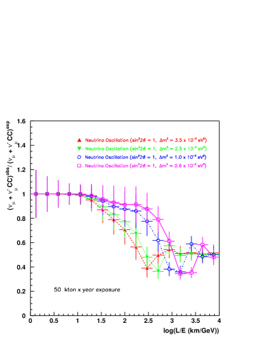
Figure 10: Survival probability as a function of the $L/E$ ratio assuming neutrino oscillation hypothesis and for various $\Delta m^{2}$ values and for 50 kton$\times$year. Only statistical error has been considered.

The most favored solution of the atmospheric neutrino anomaly is through ${\nu_{\mu}}\rightarrow{\nu_{\tau}}$ oscillations. However, alternative explanations, like neutrino decay, cannot yet be excluded decay . For example, in a model in which one of the mass-eigenstates of neutrinos with $\nu_{\mu}$ flavour content decays, the disappearance probability can be described by the expression:

$$P(\nu_{\mu}\rightarrow\nu_{x\neq\mu})=(\sin^{2}\theta+\cos^{2}\theta e^{-\alpha L/2E})^{2}.$$ (2)

Such a model gives an equally good fit for the choice of parameters $\alpha=1/63$ GeV/km, $\cos^{2}\theta=0.30$ decay .

The capability of distinguishing between the two hypothesis depends on the resolution in measuring the $L/E$ ratio, which depends on the angular and momentum resolution.

Figure 11 shows the survival probabilities as a function of $L/E$ for the neutrino decay hypothesis with $\alpha=m_{\nu}/\tau_{\nu}=1/63$ GeV/km and $\cos^{2}\theta=0.30$, and the oscillation hypothesis with $\sin^{2}2\theta=1$ and $\Delta m^{2}=1.0\times 10^{-3}$, for an exposure of 50 kton$\times$year. Both hypothesis are distinguishable from each other at around 2000 km/GeV within the statistical errors.

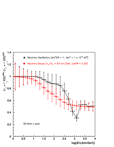
Figure 11: Survival probability as a function of the $L/E$ ratio for oscillation (triangles) and decay hypothesis (circles). Only statistical error has been considered.

5.5 (Direct) appearance of tau neutrinos

To discriminate between $\nu_{\mu}\rightarrow\nu_{\tau}$ and $\nu_{\mu}\rightarrow\nu_{s}$ oscillations, we measure the ratio $R_{NC/e}=\frac{NC^{obs}/\nu_{e}CC^{obs}}{NC^{exp}/\nu_{e}CC^{exp}}$. An oscillation to an active neutrino leads to $R_{NC/e}=1$, while $R_{NC/e}\sim 0.7$ is expected for an oscillation to sterile neutrino.

Exposure (kton$\times$year)	$R_{NC/e}$
	all events	contained
5	$0.674\pm 0.086$	$0.670\pm 0.087$
20	$0.674\pm 0.043$	$0.670\pm 0.044$
50	$0.674\pm 0.027$	$0.670\pm 0.028$

Table 9: $R_{NC/e}$ as a function of the exposure assuming oscillation to a sterile neutrino. Quoted errors are of statistical nature.

Table 9 shows values and errors of $R_{NC/e}$ in case of oscillation to a sterile neutrino, for all events and fully contained events respectively.

For $\Delta m^{2}\leq 10^{-2}$ eV², oscillations of ${\nu_{\mu}}$ into ${\nu_{\tau}}$ would in fact result in an excess of “neutral-current-like” events produced by upward neutrinos with respect to downward, since charged-current ${\nu_{\tau}}$ interactions would contribute to the “neutral-current-like” event sample, due to the large $\tau$ branching ratio into hadronic channels. Moreover, due to threshold effect on $\tau$ production, this excess would be important at high energy. Oscillations into a sterile neutrino would instead result in a depletion of upward muon-less events. Discrimination between ${\nu_{\mu}}\rightarrow{\nu_{\tau}}$ and ${\nu_{\mu}}\rightarrow\nu_{s}$ is thus obtained from a study of the asymmetry of upward to downward muon-less events. Because this method works with the high energy component of atmospheric neutrinos, it becomes effective for relatively large values of $\Delta m^{2}$ ($\geq 3\times 10^{-3}$ eV²).

Charged current $\nu_{\tau}$ rates for five $\Delta m^{2}$ hypothesis: $5\times 10^{-4}$, $1\times 10^{-3}$, $3.5\times 10^{-3}eV^{2}$, $5\times 10^{-3}eV^{2}$ and $1\times 10^{-2}eV^{2}$ are listed in Table 10. We see that the rates saturate at about one event per kton$\times$year for the larger $\Delta m^{2}$ values. Such small rates pose a major experimental challenge in the detection of $\nu_{\tau}$ in the cosmic ray induced neutrino flux.

$\nu_{\tau}+\bar{\nu}_{\tau}$ CC (NUX, Fluka 3D flux)				Rel. to	Rel. to
	Rate (kton$\times$ year)			Fluka 1D	Bartol
$\Delta m^{2}$ (eV2)	DIS	QE	Sum
$5\times 10^{-4}$	0.11	0.11	0.22	0.96	0.81
$1\times 10^{-3}$	0.28	0.18	0.46	1.02	0.84
$3.5\times 10^{-3}$	0.59	0.21	0.80	1.00	0.81
$5\times 10^{-3}$	0.64	0.24	0.88	1.01	0.80
$1\times 10^{-2}$	0.70	0.20	0.90	0.99	0.78

Table 10: Expected $\nu_{\tau}$, $\bar{\nu}_{\tau}$ absolute rates for five different $\Delta m^{2}$ with FLUKA-3D fluxes and relative to FLUKA-1D and Bartol fluxes.

The total visible energy ($E_{visible}$) is a suitable discriminant variable to enhance the $S/B$ ratio. After cuts, surviving events are classified as: $n_{b}$ (number of expected downward going background) and $n_{t}=n_{b}+n_{s}$ (number of expected upward going events, where $n_{s}$ is the number of taus). The statistical significance of the expected $n_{s}$ excess is evaluated following two procedures:

• The $f_{b}$ and $f_{t}$ pdf’s are integrated over the whole spectrum of possible measured $r$ values and the overlap between the two is computed: $P_{\alpha}\equiv\int_{0}^{\infty}min(f_{b}(r),\ f_{t}(r))dr$, where $f_{b}$ and $f_{t}$ are the Poisson p.d.f.’s for means $\mu=n_{b}$ and $\mu=n_{t}$ respectively. The smaller the overlap integrated probability ($P_{\alpha}$) the larger the significance of the expected excess.

• computing the probability $P_{\beta}\equiv\int_{n_{t}}^{\infty}\frac{e^{-n_{b}}n_{b}^{r}}{r!}dr$ that, due to a statistical fluctuation of the unoscillated data, we measure $n_{t}$ events or more when $n_{b}$ are expected.

For a 50 kton$\times$year exposure, the results of a search based on $E_{visible}$ are shown in Table 11. We see that a cut on visible energy between 6 and 7 GeV results in: (1) an overlap integrated probability between the two distributions amounting to $25-26\%$. (2) a Poisson probability that the measured excess (“$\tau$ bottom”) corresponds to a statistical fluctuation is $0.6-0.8\%$.

50 kton$\times$year exposure
$E_{Visible}cut$	$\nu$ NC top	$\tau$ bottom	$P_{\alpha}$ ($\%$)	$P_{\beta}$ ($\%$)
$>1$ GeV	327	22	55.0	10.8
$>2$ GeV	150	22	38.6	3.54
$>3$ GeV	95	21	30.6	1.6
$>4$ GeV	67	20	25.3	0.8
$>5$ GeV	51	17	27.3	0.9
$>6$ GeV	40	16	24.6	0.6
$>7$ GeV	33	14	26.6	0.8
$>8$ GeV	28	13	26.7	0.8
$>9$ GeV	23	12	26.2	0.7
$>10$ GeV	21	11	28.3	0.9

Table 11: Number of NC and tau events as a function of the visible energy cut. The statistical sample used corresponds to an exposure of 50 kton$\times$year.

The search for $\nu_{\tau}$ appearance can be improved taking advantage of the special characteristics of $\nu_{\tau}$ CC and the subsequent decay of the produced $\tau$ lepton when compared to CC and NC interactions of $\nu_{\mu}$ and $\nu_{e}$, i.e. by making use of $\vec{P}_{lepton}$ and $\vec{P}_{hadron}$.

The information related to the directionality of the incoming neutrino (i.e. the beam direction!) is missing. As a result, we have three kinematical independent variables in order to separate signal from background. After a careful evaluation of the performance of different combinations of variables, we decided to use: $E_{visible}$, $y_{bj}$ (the ratio between the total hadronic energy and $E_{visible}$), and $Q_{T}$ (the transverse momentum of the $\tau$ candidate with respect to the total measured momentum) which contains the information on the isolation of the tau candidate from the recoiling jet.

The chosen variables are not independent one from another but show correlations between them. These correlations can be exploited to reduce the background. In order to maximize the separation between signal and background, we use three dimensional likelihood functions ${\cal L}(Q_{T},E_{visible},y_{bj})$ where correlations are taken into account (see Figure 12).

Figure 12: Likelihood ratio distributions, arbitrarily normalized, for signal and background events. The distributions are computed separately for each of the considered hadronic channels: $\pi$, $\rho$, 3 prongs.

$\pi$	$\rho$	${3\pi}$	Top	Bot.	$P_{\alpha}$	$P_{\beta}$
Cut	Cut	Cut	Evts	Evts	($\%$)	($\%$)
0	0.5	0	112	$134$	32.1	$1.9$ ($2.3\sigma$)
1.5	1.5	0	46	$63$	24.8	$0.7$ ($2.7\sigma$)
3	$-1$	0	43	$59$	26.1	$0.8$ ($2.6\sigma$)
3	0.5	0	12	$23$	18.3	$0.14$ $(3.3\sigma)$
3	1.5	0	10	$20$	18.8	$0.16$ ($3.2\sigma$)
3	0.5	$-1$	30	$45$	21.9	$0.4$ ($2.9\sigma$)
3	0.5	1	9	$17$	25.9	$0.5$ ($2.8\sigma$)

Table 12: Expected background and signal events for different combinations of the $\pi$, $\rho$ and $3\pi$ analyses. The considered statistical sample corresponds to an exposure of 50 kton$\times$year.

Table 12 illustrates the statistical significance achieved by several selected combinations of the likelihood ratios for an exposure equivalent to 50 kton$\times$year. We take as the best combination the one with the lowest $P_{\alpha}$. This is achieved for the following set of cuts: $\ln\lambda_{\pi}>3$, $\ln\lambda_{\rho}>0.5$ and $\ln\lambda_{3\pi}>0$. The expected number of NC background events amounts to 12 (top) while 12+11 = 23 (bottom) are expected. This corresponds to a $P_{\alpha}$ of 18.3$\%$. In the case we consider $E_{visible}$ as the unique discriminating variable, a similar number of background events is obtained demanding $E_{visible}>14$ GeV. With this cut, the expected number of $\tau$ events is 7 and the $P_{\alpha}$ is 37$\%$. Therefore, for the same level of background, the approach using the ratio of three dimensional likelihood functions enhances the number of expected signal events by approximately 50$\%$.

Finally, in figure 13 we present the Poisson probability $P_{\beta}$ for the measured excess of upward going events to be due to a statistical fluctuation as a function of the exposure. The bottom curve corresponds to the case where no kinematical selection has been applied and only a cut on $E_{visible}>6$ GeV is used. We see that for exposures around 30 kton$\times$year, in case we use the kinematical selection algorithm, the observed excess corresponds to a 2.6$\sigma$ effect. This effect is larger than $3\sigma$ for an exposure of 50 kton$\times$year.

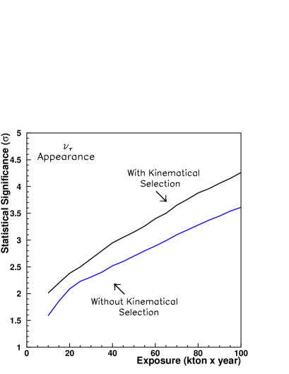
Figure 13: Probability for the measured excess of upward going events to be due to a statistical fluctuation of the data as a function of the exposure.

References

- (1) F. Arneodo et al. [ICARUS and NOE Collab.], “ICANOE: Imaging and calorimetric neutrino oscillation experiment,” LNGS-P21/99, INFN/AE-99-17, CERN/SPSC 99-25, SPSC/P314. Updated information can be found at http://pcnometh4.cern.ch.
- (2) see e.g. C. Walter [Superkamiokande Collab.], “Results from Super-Kamiokande and the status of K2K”, to appear in the Proceedings of the EPS99 conference, Tampere, Finland, 1999.
- (3) J. Altegoer et al. [NOMAD Collaboration], Phys. Lett. B431, 219 (1998).
- (4) CHORUS Collab., E. Eskut et al., Phys. Lett. B 434, 205 (1998). CHORUS Collab., E. Eskut et al., Phys. Lett. B 424, 202 (1998).
- (5) ICARUS Web page: http://www.aquila.infn.it/icarus./
- (6) NOE Web page: http://www.na.it/NOE/
- (7) A. Bueno, M. Campanelli, A. Ferrari, A. Rubbia, “Nucleon Decay studies in a large Liquid Argon detector”, these proceedings.
- (8) G. Acquistapace et al., CERN 98-02 and INFN/AE-98/05; R. Bailey et al., CERN-SL/99-034(DI) and INFN/AE-99/05
-
(9)
G. Battistoni, A. Ferrari, P. Lipari, T. Montaruli,
P.R. Sala and T. Rancati, “A 3–Dimensional Calculation of
Atmospheric Neutrino Flux ” hep-ph/9907408, submitted to Astroparticle Physics. - (10) V. Barger et al., hep-ph/9907421; V. Barger et al., Phys. Rev. Lett. 82 (1999) 2640.