Laser cooling of electron beams at linear colliders.

Abstract

A method of electron beam cooling is considered which can be used for linear colliders. The electron beam is cooled during collision with focused powerful laser pulse. The ultimate transverse emittances are much below those achievable by other methods. This method is especially useful for high energy gamma-gamma colliders. In this paper we review and analyse limitations in this method, also discuss a new method of obtaining very high laser powers required for the laser cooling, radiation conditions and finaly present a possible scheme for the laser cooling of electron beams.

1 Introduction, one pass laser cooling

To explore the energy region beyond LEP-II, linear colliders (LC) with center–of–mass energy 0.5–2 TeV are developed now in the main accelerator centers [1],[2],[3]. Besides e⁺e^- collisions, at linear colliders one can “convert” electrons to high energy photons using the Compton backscattering of laser light, thus obtaining $\gamma\gamma$ and $\gamma e$ collisions with energies and luminosities close to those in e⁺e^- collisions [4]-[13].

To attain high luminosity, beams in linear colliders should be very tiny. At the interaction point (IP) in the current LC designs, beams with transverse sizes as low as $\sigma_{x}$/$\sigma_{y}$ $\sim$ 300/3 nm are planned. Beams for e⁺e^- collisions should be flat in order to reduce beamstrahlung energy loss. For $\gamma\gamma$ collision, the beamstrahlung radiation is absent also there are no beam instabilities therefore beams with smaller $\sigma_{x}$ ($\sigma_{x}/\sigma_{y}\sim 10/1$ nm) can be used [14],[11]-[13] to obtain higher luminosity.

The transverse beam sizes are determined by the emittances $\epsilon_{x}$, and $\epsilon_{y}$. The beam sizes at the interaction point (IP) are $\sigma_{i}=\sqrt{\mbox{$\epsilon_{i}$}\ \mbox{$\beta_{i}$}\ }$, where $\beta_{i}$ is the beta function at the IP. With the increase of the beam energy the emittance of the bunch decreases: $\mbox{$\epsilon_{i}$}=\mbox{$\epsilon_{ni}$}/\gamma$, where $\gamma=E/mc^{2},$ $\epsilon_{ni}$ is the normalized emittance.

The beams with a small $\epsilon_{ni}$ are usually prepared in damping rings which naturally produce bunches with $\mbox{$\epsilon_{ny}$}\ll\mbox{$\epsilon_{nx}$}$ [15]. Laser RF photoguns can also produce beams with low emittances [16]. However, for linear colliders it is desirable to have smaller emittances.

Recently, a new method of electron beam cooling was proposed which allows further reduction of the transverse emittances after damping rings or guns by 1–3 orders of magnitude [17],[18].

The idea of laser cooling of electron beams is very simple, see fig. 1.

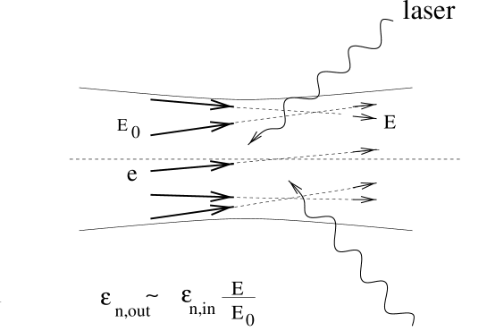
Figure 1: Principle of the laser cooling.

During head-on collisions with optical laser photons (with an electromagnetic wave in the case of a very strong field) the transverse distribution of electrons ($\sigma_{i}$) remains almost unchanged. Also the angular spread ($\sigma_{i}^{\prime}$) is almost constant, because for photon energies (a few eV) much lower than the electron beam energy (several GeV) the scattered photons follow the initial electron trajectory with a small additional spread. So, the emittance $\mbox{$\epsilon_{i}$}=\mbox{$\sigma_{i}$}\mbox{$\sigma_{i}^{\prime}$}$ remains almost unchanged. At the same time, the electron energy decreases from $E_{0}$ down to $E$. This means that the transverse normalized emittances have decreased: $\mbox{$\epsilon_{n}$}=\gamma\mbox{$\epsilon$}=\mbox{$\epsilon_{n}$}_{0}(E/E_{0})$. One can reaccelerate the electron beam up to the initial energy and repeat the procedure. Then after N stages of cooling $\mbox{$\epsilon_{n}$}/\mbox{$\epsilon_{n}$}_{0}=(E/E_{0})^{N}$ (if $\epsilon_{n}$ is far from its limit).

The ultimate emittance can be estimated in the following way. In the electron beam reference system the counter moving laser photons have an energy $\omega\sim\gamma\omega_{0}$ ($\gamma=E/mc^{2}$ and $\omega_{0}$ is the energy of laser photons) and scatter almost isotropically (roughly) without change of the energy. As a result, after multiple Compton scattering, the transverse energy of the electrons is equal to the transverse energy of laser photons

$$p_{t}^{2}/m\sim\gamma\omega_{0}.$$ (1)

Here we assumed that $\gamma\omega_{0}\ll mc^{2}$. On the other hand the r.m.s. angular spread of the electrons in the laboratory system by definition (see above)

$$\frac{p_{t}}{\gamma mc}\equiv\sqrt{\frac{\mbox{$\epsilon_{n}$}}{\gamma\beta}},$$ (2)

where $\epsilon_{n}$ is the normalized emittance and $\beta$ is the beta-function of the electron beam in the cooling region. Substituting eq.1 to eq.2 we obtain

$$\mbox{$\epsilon_{n}$}\ \sim\frac{\lambda_{C}}{\lambda}\beta,$$ (3)

where $\lambda_{C}=\hbar/mc$ is the Compton wave length, $\lambda$ is the laser wave length.

The physics of the cooling process is almost the same as radiative cooling of electrons in damping rings. However, here the process takes only 1 ps and the ultimate emittance is much lower than that in the damping rings. This is because in the “linear” laser cooling there are no bends (as in damping rings) which cause a growth of the horizontal emittance. Also the intra-beam scattering is not important due to a short “damping” time and following fast acceleration.

There are several question to this method

1. requirements for laser parameters (these parameters should be attainable);

2. an energy spread of the beam after cooling (at the final energy of a linear collider it is necessary to have $\sigma_{E}/E\sim 0.1\%$; also with a large energy spread it is difficult to “match” the cooled beam with the accelerator due to the chromaticity of focusing systems and also to focus the beams for the next stage of cooling.)

3. the limit on the final normalized emittances (it is desirable to have this limit lower than that obtained with storage rings and photoguns);

4. depolarization of electron beams (polarization is very important for linear colliders).

5. radiation damage of mirrors by the photons scattered at the large angles (these are X-ray photons).

Below we will see that this method is perfectly suited for linear colliders, however the main problem here obtaining of a very powerful laser pulses with high repetition rate. On my opinion, the most promising approach to this problem is a pulse stacking of laser pulses in an optical cavity [12],[20]. All these problems and possible solutions are discussed below.

2 Flash energy.

In the cooling region, a laser photon with energy $\omega_{0}$ (wave length $\lambda$) collides almost head–on with an electron of energy $E$. The kinematics is determined by two parameters $x$ and $\xi$ [5, 7, 8]. The first one

$$x=\frac{4E\omega_{0}}{m^{2}c^{4}}=0.019\left[\frac{E}{\mbox{GeV}}\right]\left[\frac{\mbox{$\mu$m}}{\lambda}\right]$$ (4)

determines the maximum energy of the scattered photons:

$$\omega_{m}=Ex/(x+1)\sim 4\gamma^{2}\omega_{0}\;\;\;\;(x\ll 1).$$ (5)

If the electron beam is cooled at the initial energy $E_{0}=5\;\mbox{GeV}$ (after damping ring and bunch compression) and $\lambda=0.5\;\mbox{$\mu$m}$ (Nd:glass laser) then $x_{0}\simeq 0.2$ (we will provide $E$ and $x$ with the index 0 for designation of their values at the begining of a cooling region).

For our further consideration we will need also the following formulae for the Compton scattering in the case $x<<1$. The energy spectrum of scattered photons(normalized per one scattering) [5]

$$dp=(3/2)[1-2\omega/\omega_{m}+2(\omega/\omega_{m})^{2}]d\omega/\omega_{m}.$$ (6)

The angle of the electron after scattering

$$\theta_{1}^{2}=(\omega_{m}\omega-\omega^{2})/(\gamma^{2}E^{2}).$$ (7)

The second parameter characterizes a strength of an electromagnatic wave

$$\xi^{2}=\left(\frac{eB_{0}\hbar}{m\omega_{0}c}\right)^{2},$$ (8)

where $B_{0}$ is the magnetic (or electric) field strength in the laser wave. At $\xi^{2}\ll 1$ an electron interacts with one photon from the field (Compton scattering, undulator radiation), while at $\xi^{2}\gg 1$ an electron scatters on many laser photons simultaneously (synchrotron radiation (SR), wiggler). We will see that in the considered method $\xi^{2}$ may be “small” and “large”.

In the cooling region near the laser focus the r.m.s radius of the laser beam depends on the distance $z$ to the focus (along the beam) in the following way [5]: $r_{\gamma}=a_{\gamma}\sqrt{1+z^{2}/Z_{R}^{2}}$, where $Z_{R}=2\pi a^{2}_{\gamma}/\lambda$ is the Rayleigh length (an effective depth of laser focus), $a_{\gamma}$ is the r.m.s. focal spot radius. The density of laser photons is $n_{\gamma}=(A/\pi r^{2}_{\gamma}\omega_{0})\exp(-r^{2}/r^{2}_{\gamma})F_{\gamma}(z+ct)$, where $A$ is the laser flash energy and $\int F_{\gamma}(z)dz=1.$

In the case of strong field ($\xi^{2}\gg 1$) it is more appropriate to speak in terms of strength of the electromagnetic field which is $\bar{B^{2}}/4\pi=n_{\gamma}\omega_{0},B=B_{0}cos(\omega_{0}t/\hbar-kz)$. Assuming $F_{\gamma}=1/l_{\gamma}$ and $Z_{R}\ll l_{\gamma}\simeq l_{e}$ and using the classical formula for radiation loss ($dE/dx=(2/3)r^{2}_{e}\gamma^{2}B^{2},\;r_{e}=e^{2}/mc^{2}$) we obtain the ratio of emittances before and after the laser target

$$\frac{\mbox{$\epsilon_{n}$}_{0}}{\mbox{$\epsilon_{n}$}}\simeq\frac{E_{0}}{E}=1+\frac{r_{e}^{2}}{3m^{2}c^{4}}\int B_{0}^{2}dz=1+\frac{64\pi^{2}r_{e}^{2}\gamma_{0}}{3mc^{2}\lambda\l_{e}}A\$$ (9)

$$A[J]=\frac{25\lambda[\mbox{$\mu$m}\ ]l_{e}[\mbox{mm}\ ]}{E_{0}[\mbox{GeV}\ ]}\left(\frac{E_{0}}{E}-1\right).$$ (10)

These equations are correct at $x\ll 1$ for any value of $\xi^{2}$. For example: at $\lambda=0.5\;\mbox{$\mu$m},\;l_{e}=0.2\;\mbox{mm},E_{0}=5\;\mbox{GeV},E_{0}/E=10$ the required laser flash energy $A=4.5\;J.$ To reduce the laser flash energy in the case of long electron bunches, one can compress the bunch (length) before cooling as much as possible and stretch it after cooling up to the required value.

The eqs.9,10 were obtained for $Z_{R}\ll l_{\gamma}\sim l_{e}$ and give the minimum flash energy for a certain ratio $E_{0}/E$. To further estimate the photon density at the laser focus we will assume $Z_{R}\sim 0.25l_{e}$. In this case, the required flash energy is still close to its minimum, but the field strength is not so high as for very small $Z_{R}$. From the previous equation for $Z_{R}=0.25l_{e}$ it follows $B_{0}^{2}/(8\pi)=\omega_{0}n_{\gamma}=A/(\pi a_{\gamma}^{2}l_{e})=8A/(\lambda l_{e}^{2})$. Substituting $B_{0}$ into eq.8 we get

$$\xi^{2}=\frac{16r_{e}\lambda A}{\pi l_{e}^{2}mc^{2}}=\frac{3\lambda^{2}}{4\pi^{3}r_{e}l_{e}\gamma_{0}}\left(\frac{E_{0}}{E}-1\right)\ ==4.3\frac{\lambda^{2}[\mbox{$\mu$m}\ ]}{l_{e}[\mbox{mm}\ ]E_{0}[\mbox{GeV}\ ]}\left(\frac{E_{0}}{E}-1\right).$$ (11)

Example: for $\lambda$ = 0.5 $\mu$m, $E_{0}$ = 5 GeV , $E_{0}/E$ = 10, $l_{e}$ = 0.2 mm (the NLC project) $\Rightarrow\xi^{2}$ = 9.7. For larger bunch lengths and shorter wave lengths, $\xi^{2}$ may be smaller. So, both ”undulator” and ”wiggler” cases are possible.

Later we will see that in order to have lower limit on emittance and smaller depolarization it is necessary to have a low $\xi^{2}$. With a usual optics one can reduce $\xi^{2}$ only by increasing $l_{\gamma}$ (and $Z_{R}$) with a simultaneous increase of the laser flash energy. From (10) and (11) we get

$$A\propto\frac{\lambda^{3}}{\gamma_{0}^{2}\xi^{2}}\left(\frac{E_{0}}{E}-1\right)^{2}.$$ (12)

Is it possible to reduce $\xi^{2}$ keeping all other parameters (including flash energy) constant? Yes, providing a way to stretch the focus depth without changing the radius of this area is found. In this case, the collision probability (or $\int B^{2}dz$) remains the same but the maximum value of $\xi^{2}$ will be smaller. A solution of this problem was given in [17]. It is based on the non-monochromaticity of the laser light and the chirped pulse technique. In this scheme, the cooling region consists of many laser focal points (continuously) and light comes to each point exactly at the moment when the electron bunch is there. One can consider that a short electron bunch collides on its way sequentially with $n_{f}$ (“number of focuses”) short light pulses of length $l_{\gamma}\sim l_{e}$ and focused with $2Z_{R}\sim l_{e}$. There is one restriction on $n_{f}$: along the cooling length $L\approx\mbox{$n_{f}$}\cdot l_{e}$ the transverse size of an electron beam should be smaller than the laser spot size $a_{\gamma}\simeq\sqrt{\lambda Z_{R}/2\pi}\sim\sqrt{\lambda l_{e}/4\pi}$. In further examples we will use $\mbox{$n_{f}$}\ \sim 10$ for stretching the cooling region from 100 $\mu$m to 1 mm.

Other method of “stretching” is using of several lasers focused to different, though this require larger flash energy (see sect.10).

3 Energy spread

The electron energy spread arises from the quantum-statistical nature of radiation. After energy loss $\Delta E$, the increase of the energy spread $\Delta(\sigma_{E}^{2})=\int\varepsilon^{2}\dot{n}(\omega)d\omega dt=-aE^{2}\Delta E$, where $\dot{n}(\omega)$ is the spectral density of photons emitted per unit time, $a=14\omega_{0}/5m^{2}c^{4}=7x_{0}/10E_{0}$ for the Compton case and $a=55\hbar eB_{0}/(8\pi\sqrt{3}m^{3}c^{5})\;$ for the “wiggler” case.

There is the second effect which leads to decreasing the energy spread. It is due to the fact that $dE/dx\propto E^{2}$ and an electron with higher (lower) energy than the average loses more (less) than on average. This results in the damping: $d(\sigma_{E}^{2})/\sigma_{E}^{2}=4dE/E$ (here $dE$ has negative sign). The full equation for the energy spread is $d\sigma_{E}^{2}=-aE^{2}dE+4(dE/E)\sigma_{E}^{2}$, with solution $\sigma_{E}^{2}/E^{2}=\sigma_{E_{0}}^{2}E^{2}/E_{0}^{4}+aE_{0}(E/E_{0})(1-E/E_{0})$. In our case

$$\frac{\sigma_{E}^{2}}{E^{2}}\sim\frac{\sigma_{E_{0}}^{2}E^{2}}{E_{0}^{4}}+\frac{7}{10}x_{0}(1+\frac{275\sqrt{3}}{336\pi}\xi)\frac{E}{E_{0}}\left(1-\frac{E}{E_{0}}\right),$$ (13)

here the results for the Compton scattering and SR are joined together. Example: at $\lambda=0.5\;\mbox{$\mu$m},\;E_{0}=5\;\mbox{GeV}\ (x_{0}=0.19)$ and $E_{0}/E=10$, the Compton term alone gives $\sigma_{E}/E\sim 0.11$ and with the “wiggler” term ($\xi^{2}=9.7$, see the example above) $\sigma_{E}/E\sim 0.17$. What $\sigma_{E}/E$ is acceptable? In the last example $\sigma_{E}/E\sim 0.17$ at E = 0.5 GeV (after cooling). This means that at the collider energy E = 250 GeV we will have $\sigma_{E}/E\sim 0.034\%$, that is better than necessary (about 0.1 %).

In a two stage cooling system, after reacceleration to the initial energy $E_{0}$ = 5 GeV the energy spread is $\sigma_{E}/E_{0}\sim 1.7\%$. For this value there may be a problem with focusing of electrons which can be solved using a focusing scheme with correction of chromatic aberrations. It is even more difficult to “match” the electron beam after the laser cooling with the accelerator (see sect.9.

4 Minimum normalize emittance.

It is determined by the quantum nature of the radiation. Let us start with the case of pure Compton scattering at $\xi^{2}\ll 1$ and $x_{0}\ll 1$. In this case, the scattered photons have the energy distribution given by eq.6 The angle of the electron after scattering is connected with the energy by eq.7. After averaging over the energy spectrum we get the average $\theta_{1}^{2}$ in one collision: $\langle\theta_{1}^{2}\rangle=12\omega_{0}^{2}/(5m^{2}c^{4})$. After many Compton collisions ($N_{coll}$) the r.m.s. angular spread in i=x,y projection $\Delta\langle\theta^{2}_{i}\rangle=0.5\Delta\langle\theta^{2}\rangle=0.5N_{coll}\langle\theta_{1}^{2}\rangle=-0.5(\Delta E/\bar{\omega})\langle\theta_{1}^{2}\rangle=-3\omega_{0}\Delta E/5E^{2}$.

The normalized emittance $\mbox{$\epsilon_{ni}$}{{}^{2}}=(E^{2}/m^{2}c^{4})\langle r_{i}^{2}\rangle\langle\theta_{i}^{2}\rangle$ does not change when $\Delta\langle\theta_{i}^{2}\rangle/\langle\theta_{i}^{2}\rangle$ = $-2\Delta E/E.$ Taking into account that $\langle\theta_{i}^{2}\rangle\equiv\mbox{$\epsilon_{ni}$}\ /\gamma\beta_{i}$ we get the equilibrium emittance due to the Compton scattering

$$\mbox{$\epsilon_{ni}$}_{,min}\approx 0.5\gamma E\beta_{i}\Delta\langle\theta_{i}^{2}\rangle/\Delta E=\frac{3\pi}{5}\frac{\lambda_{c}}{\lambda}\beta_{i}=\frac{7.2\times 10^{-10}\beta_{i}[mm]}{\lambda[\mbox{$\mu$m}\ ]}\;\;\mbox{m$\cdot$rad},$$ (14)

where $\lambda_{c}=\hbar/mc$. For example: $\lambda=0.5\;\mbox{$\mu$m},\;\beta=l_{e}/2=0.1\;\mbox{mm}\ ($NLC$)\Rightarrow\mbox{$\epsilon_{n}$}_{,min}=1.4\times 10^{-10}\;\mbox{m}\cdot$rad. For comparison in the NLC project the damping rings have $\mbox{$\epsilon_{nx}$}\ =3\times 10^{-6}\;\mbox{m}\cdot$rad, $\mbox{$\epsilon_{ny}$}\ =3\times 10^{-8}\;\mbox{m}\cdot$rad.

If $\xi^{2}\gg 1$, the electron moves as in a wiggler.Assume that the “laser wiggler” is planar and deflects the electron in the horizontal plane. If an electron with energy E emits a photon with energy $\omega$ along its trajectory the emittance changes as follows [15]: $\delta\mbox{$\epsilon_{x}$}=(\omega^{2}/2E^{2})H(s);\;H(s)=\beta_{x}\eta_{x}^{\prime 2}+2\alpha_{x}\eta_{x}\eta_{x}^{\prime}+\gamma_{x}\eta_{x}^{2}$; where $\alpha_{x}=-\beta_{x}^{\prime}/2,\;\gamma_{x}=(1+\alpha_{x}^{2})/\beta_{x},\;\beta_{x}$ is the horizontal beta-function, $\eta_{x}$ is the dispersion function, $s$ is the coordinate along the trajectory. For $\beta_{x}=const$ the second term in H is equal to zero, the second term in a wiggler with $\lambda_{w}\ll\beta$ is small, so that H(s) $\approx\beta\eta^{\prime 2}$. In a sinusoidal wiggler field $B(z)=B_{w}cos\;k_{w}z,\;k_{w}=2\pi/\lambda_{w}$, $\eta^{\prime\prime}=1/\rho$ ($\rho$ is the radius of curvature) one finds that $\eta^{\prime}=(eB_{w}/k_{w}E)\;sin\;k_{w}z$. The increase of $\epsilon_{x}$ on a distance $dz$ is

$$\Delta\mbox{$\epsilon$}_{x}=\int\frac{H}{2}\left(\frac{\omega}{E}\right)^{2}\dot{n}(\omega)d\omega dt=\frac{55}{48\sqrt{3}}\frac{r_{e}\hbar c}{(mc^{2})^{6}}E^{5}\langle\frac{{\it H}}{\rho^{3}}\rangle dz,$$ (15)

where $\langle{\it H}/\rho^{3}\rangle_{w}=8\beta_{x}\lambda_{w}^{2}(eB_{w})^{5}/(140E^{5}\pi^{3})$ for the wiggler and $\dot{n}(\omega)$ is the spectral density of photons emitted per unit time. The energy loss averaged over the wiggler period is $\Delta E=r_{e}^{2}B_{w}^{2}E^{2}dz/(3m^{2}c^{4})$. The normalized emittance $\mbox{$\epsilon_{n}$}=\gamma\mbox{$\epsilon$}\$ is not changed when $Ed\mbox{$\epsilon$}\ +\mbox{$\epsilon$}\ dE=0$. Using this and replacing $B_{w}$ by 2$B_{0}$, $\lambda_{w}$ by $\lambda/2$ we obtain the equilibrium normalized emittance in the linear polarized electromagnatic wave for $\xi^{2}\gg 1$

$$\mbox{$\epsilon_{nx}$}=\frac{11e^{3}\hbar c\lambda^{2}B_{0}^{3}\beta_{x}}{24\sqrt{3}\pi^{3}(mc^{2})^{4}}=\frac{11}{3\sqrt{3}}\frac{\lambda_{C}}{\lambda}\beta_{x}\xi^{3}\approx\frac{8\cdot 10^{-10}\beta_{x}[\mbox{mm}\ ]\xi^{3}}{\lambda[\mbox{$\mu$m}\ ]}\;\;\mbox{m$\cdot$rad}.$$ (16)

Using eq.11 we can get a scaling of the minimum $\epsilon_{nx}$ for a multistage cooling system with a cooling factor $E_{0}/E$ in one stage: $\mbox{$\epsilon_{nx}$}\ \propto\beta_{x}\lambda^{2}(E_{0}/E)^{3/2}/(l_{e}\gamma_{0})^{3/2}$ when $l_{\gamma}\sim l_{e}$(minimum A) and $\mbox{$\epsilon_{nx}$}\ \propto\beta_{x}\lambda^{7/2}(E_{0}/E)^{3}/(\gamma_{0}^{3}A^{3/2})$ for free A and $\l_{\gamma}>l_{e}$ (for $\beta_{x}=const$). Stretching the laser focus depth by a factor $n_{f}$ , one can further reduce the horizontal normalized emittance: $\mbox{$\epsilon_{nx}$}\ \propto 1/\mbox{$n_{f}$}^{1/2}$(if $\beta_{x}\propto\mbox{$n_{f}$}$). For our previous example we have $\xi^{2}=9.7$ and $\mbox{$\epsilon_{nx}$}\ =5\cdot 10^{-9}\;\mbox{m}\cdot$rad (in the NLC $\epsilon_{nx}$ = 3$\cdot 10^{-6}$ m$\cdot$rad). Stretching the cooling region with $n_{f}$=10, further decreases the horizontal emittance by a factor 3.2.

Comparing with the Compton case (14) we see that in the strong field the horizontal emittance is larger by a factor $\xi^{3}$. The origin of this factor is clear: $\mbox{$\epsilon_{nx}$}\propto\eta_{x}^{\prime 2}\omega_{crit.}$, where $\eta_{x}^{\prime}\sim\xi\theta_{compt.}$ and $\omega_{crit.}\sim\xi\omega_{compt.}$.

Let us roughly estimate the minimum vertical normalized emittance at $\xi\gg\ 1$. Assuming that all photons are emitted at an angle $\theta_{y}=1/(\sqrt{2}\gamma)$ with the $\omega=\omega_{c}$ similarly to the Compton case, one gets $\Delta\langle\theta^{2}_{y}\rangle=(\omega_{c}\Delta E)/(2\gamma^{2}E^{2})=-(3e\hbar\bar{B_{w}}\Delta E)/(4E^{2}mc)$. Using the first part of eq.14 we get

$$\mbox{$\epsilon_{ny}$}_{min}\sim\frac{3}{8}\frac{\hbar e\bar{B_{w}}}{m^{2}c^{3}}\beta_{y}=3\left(\frac{\lambda_{C}}{\lambda}\right)\beta_{y}\xi\approx\frac{1.2\cdot 10^{-9}\beta_{y}[\mbox{mm}\ ]\xi}{\lambda[\mbox{$\mu$m}\ ]}\;\;\mbox{m$\cdot$rad}.$$ (17)

For the previous example (NLC beams), eq.17 gives $\mbox{$\epsilon_{ny}$}_{min}\sim 7.5\cdot 10^{-10}$ m$\cdot$rad (for comparison in the NLC project $\mbox{$\epsilon_{ny}$}=3\cdot 10^{-8}$ m$\cdot$rad). The scaling: $\mbox{$\epsilon_{ny}$}\ \propto\beta_{y}(E_{0}/E)^{1/2}/(l_{e}\gamma_{0})^{1/2}$ when $l_{\gamma}\sim l_{e}$(minimum A) and $\mbox{$\epsilon_{ny}$}\ \propto\beta_{y}\lambda^{1/2}(E_{0}/E)/(\gamma_{0}A^{1/2})$ for free A and $\l_{\gamma}>l_{e}.$

For arbitrary $\xi$ the minimum emittances can be estimated as the sum of (14) and (16) for $\epsilon_{nx}$ and sum of (14) and (17) for $\epsilon_{ny}$

$$\mbox{$\epsilon_{nx}$}\approx\frac{3\pi}{5}\frac{\lambda_{C}}{\lambda}\beta_{x}(1+1.1\xi^{3});\;\;\mbox{$\epsilon_{ny}$}\sim\frac{3\pi}{5}\frac{\lambda_{C}}{\lambda}\beta_{y}(1+1.6\xi).$$ (18)

5 Depolarization

Finally, let us consider the problem of the depolarization. For the Compton scattering the probability of spin flip in one collision is $w=(3/40)x^{2}$ for $x\ll 1$ (it follows from formulae of ref.[22]). The average energy losses in one collision are $\bar{\omega}=0.5xE$. The decrease of polarization degree after many collisions is $dp=2wdE/\bar{\omega}=(3/10)x(dE/E)=(3/10)x_{0}(dE/E_{0})$. After integration, we obtain the relative decrease of the longitudinal polarization $\zeta$ during one stage of the cooling (at $E_{0}/E\gg 1$)

$$\Delta\zeta/\zeta=0.3x_{0}\;\;\;\propto E_{0}/\lambda,$$ (19)

For $\lambda=0.5\;\mbox{$\mu$m}\$ and $E_{0}=5\;\mbox{GeV}\$, we have $x_{0}=0.19$ and $\Delta\zeta/\zeta=5.7\%$. This is valid only for $\xi^{2}\ll 1.$

In the case of strong field ($\xi^{2}\gg 1$) the spin flip probability per unit time is the same as in the uniform magnetic field [21] $w=(35\sqrt{3}r_{e}^{3}\gamma^{2}ce\bar{B^{3}})/(144\alpha(mc^{2})^{2})$, where for the wiggler $\bar{B^{3}}=(4/3\pi)B_{w}^{3}$. Using the relation between $dE$ and $dt$ in the wiggler we get

$$\frac{\Delta\zeta}{\zeta}=\int\frac{35\sqrt{3}er_{e}B_{0}}{9\pi\alpha(mc^{2})^{2}}dE\sim\frac{35\sqrt{3}}{36\pi}x_{0}\xi.$$ (20)

For the general case, the depolarization can be estimated as the sum of equations (19) and (20)

$$\Delta\zeta/\zeta\approx 0.3x_{0}(1+1.8\xi).$$ (21)

For the previous example with $\xi^{2}=9.7$ and $x_{0}=0.19$ we get $\Delta\zeta/\zeta=0.057+0.32=0.38$, that is not acceptable. This example shows that the depolarization effect imposes very demanding requirements on the parameters of the cooling system. The main contribution to depolarization gives the second term. Stretching the cooling region by a factor of ten we can get $\Delta\zeta/\zeta=0.057+0.1\sim 15\%$.

6 Ponderomotive forces.

It is well known that in a non-uniform oscillating field an avarage force acting on a particle is non-zero, this is so called ponderomotive force. This force leads to the repulsion of the electrons from the laser focus. This effect was not described in my first paper on laser cooling [17], but it was checked that it is not essential for the considered examples. Nevertheless, it is important, especially for low beam energies, let us consider this effect in more details.

The total force acting on an electron colliding head-on with a laser wave 

$$F=2eE_{0}(x)\sin{2\omega_{0}t}=2e(E_{0}+\frac{\partial E_{0}}{\partial x}x)\sin{2\omega_{0}t}.$$ (22)

Substituting $x\approx-(eE_{0}/2\gamma m\omega_{0}^{2})\sin{2\omega_{0}t}$ we get

$$F=2e(E_{0}-\frac{e}{2\gamma m\omega_{0}^{2}}\frac{\partial E_{0}}{\partial x}E_{0}\sin{2\omega_{0}t})\sin{2\omega_{0}t}.$$ (23)

After averaging over time we get the ponderomotive force

$$\bar{F}=-\frac{e^{2}}{4\gamma m\omega_{0}^{2}}\frac{\partial E_{0}^{2}}{\partial x}=-\frac{\partial U_{eff}}{\partial x},$$ (24)

where the effective potential

$$U_{eff}=\frac{mc^{2}}{4\gamma}\xi^{2}.$$ (25)

Particle move in the direction with the minimum ponential, in our case the electrons are repulsing from the laser target. Note, that in all considerations we assume a linearly polarized laser light with $\vec{E}$ laying in the horizontal plane. In this case there are forces only in the horizontal direction.

Let us assume that the laser spot size is about a factor of 2 larger than the horizontal size of the electron beam in the laser focus, then $\partial\xi^{2}/\partial x\sim\xi^{2}/2\sigma_{x,L}$. The deflection angle on the cooling length $l_{c}$

$$\Delta\vartheta\sim\frac{p_{t}}{p}\sim\frac{F(l_{c}/c)}{\gamma mc}\sim\frac{\xi^{2}l_{c}}{8\gamma^{2}\sigma_{x,L}}.$$ (26)

The ponderomotive forces are not important if this angle is smaller than the angular spread of the electrons in the cooling region: $\Delta\vartheta<\sqrt{\mbox{$\epsilon_{nx}$}\ /\gamma\beta}$. This gives the minimum normalized horizontal emittance when ponderomotive forces are still not important

$$\mbox{$\epsilon_{nx}$}_{,min}\sim\frac{\xi^{4}l_{c}^{2}}{64\gamma^{3}\sigma^{2}_{x,L}}\beta.$$ (27)

We have seen before that the cooling by a factor of ten can be done at $\xi^{2}\sim 1$ on the length $l_{c}\sim$ 1 mm. The minimum laser spot size $\sigma_{x,L}\sim\sqrt{\lambda Z_{R}/4\pi}\sim 2.5$ $\mu$m at $\lambda=0.5$ $\mu$m and $Z_{R}\sim\sigma_{z,e}\sim 0.1$ mm. Note, that for the first stages of cooling after the damping ring the minimum $\sigma_{x,L}$ is determined by the electron beam size and should be larger by a factor of 3 than this estimate. Now we investigate the minimum emittance therefore let us take $\sigma_{x,L}=2.5$ $\mu$m. Substituting this number to eq.27 and we get for $E=500$ GeV (the minimum energy in the cooling process) the estimate of the minimum normalized emittance when ponderomotive forces are still not important

$$\mbox{$\epsilon_{nx}$}_{min}\sim 2.5\times 10^{-9}\beta[\mbox{mm}]\;\;\mbox{m$\cdot$rad}$$ (28)

This is exectly equal to the limit on the emittance in the laser cooling obtained in the previous sections. So, at the chosen beam energies the ponderomotive forces still do not limit the minimum emittance in the laser cooling, but they will be important at the lower beam energies.

7 Some ”intermediate” conclusions.

Before considering “technical” aspects in the laser cooling we can summarize the results of the previous section as a possible ”optimistic” set of parameters for the laser cooling: $E_{0}=4.5$ GeV, $l_{e}=0.2$ mm, $\lambda=0.5$ $\mu$m, flash energy $A\sim 10$ J, focusing system with stretching factor $n_{f}$=10. The final electron bunch will have an energy of 0.45 GeV with an energy spread $\sigma_{E}/E\sim 13\%$, the normalized emittances $\epsilon_{nx}$,$\epsilon_{ny}$ are reduced by a factor 10, the limit on the final emittance is $\mbox{$\epsilon_{nx}$}\ \sim\mbox{$\epsilon_{ny}$}\ \sim 2\times 10^{-9}\;$ m$\cdot$rad at $\beta_{i}=1\;\mbox{mm}$, depolarization $\Delta\zeta/\zeta\sim 15\%$. The two stage system with the same parameters gives 100 times reduction of emittances (with the same limits).

For the cooling of the electron bunch train one laser pulse can be used many times. According to (10) $\Delta E/E=\Delta A/A$ and even 25% attenuation of laser power leads only to small additional energy spread.

8 Laser systems

We have seen that the “very” minimum flash energy required for the one stage of the laser cooling is about 10 J for visible light and $E\sim 5$ GeV beam energy. If $\lambda\sim 1$ $\mu$m (most powerful solid state lasers) then $A\sim 20$ J. If the electron beam is somewhat longer than in the considered examples, say $\sigma_{z}=$ 300-400 $\mu$m as in the TESLA project, then the required flash is already $\sim$ 40–50 J. Beside, as we will see in the next section, for decreasing the radiation damage of the mirrors one has to put the mirrors far enough from the electron beam. That leads already to more than 100 J flash energies. Moreover, the repetition rate should be equal to the rep.rate of linear colliders which is of the order of 10 kHz. So, the average power of the laser system should be of the order of one MegaWatt! At present, the best short pulse laser systems can produce several Joule pulses with the repetition rate several Hz and only there are hopes that next year a commercial 100 W laser with short (ps) pulses will be built [1],[23]. However, the situation is not so pessimistic.

To overcome the “repetition rate” problem it is quite natural to consider a laser system where one laser bunch is used for e$\to\gamma$ conversion many times. Indeed, one Joule laser flash contains about $10^{19}$ laser photons and only $10^{12}$ photons are knocked out in the collision with one electron bunch ($\sim 100$ Compron scattering per one electron).

The simplest solution is to trap the laser pulse to some optical loop and use it many times. [1] In such a system the laser pulse enters via the film polarizer and then is trapped using Pockels cells and polarization rotating plates. Unfortunately, such a system will not work with Terawatt laser pulses due to a self-focusing effect.

Fortunately, there is one way to “create” a powerful laser pulse in the optical “trap” without any “nonlinear” material inside (only very thin dielectric coating of mirrors). This very promising technique is discussed below.

8.1 Laser pulse stacking in an “external” optical cavity.

Shortly, the method is the following. Using the train of low energy laser pulses one can create in the external passive cavity (with one mirror having some small transparency) an optical pulse of the same duration but with much higher energy (pulse stacking). This pulse circulates many times in the cavity each time colliding with electron bunches passing the center of the cavity.

The idea of pulse stacking is simple but not trivial and not well known. This method is used now in several experiments on detection of gravitation waves. In my opinion, pulse stacking is very natural for photon colliders and allows not only to build a relatively cheap laser system for $e\to\gamma$ conversion but gives us the practical way for realization of laser cooling, i.e. opens up the way to ultimate luminosities of photon colliders.

As this method is very important (may be crucial) for the laser cooling, let me explain it in more detail [12],[24]. The principle of pulse stacking is shown in Fig.2.

Figure 2: Principle of pulse stacking in an external optical cavity.

The secret consists in the following. There is a well known optical theorem: at any surface, the reflection coefficients for light coming from one and the other sides have opposite signs. In our case, this means that light from the laser entering through semi-transparent mirror into the cavity interferes with reflected light inside the cavity constructively, while the light leaking from the cavity interferes with the reflected laser light destructively. Namely, this fact produces asymmetry between cavity and space outside the cavity!

Let R be the reflection coefficient, T the transparency coefficient and $\delta$ the passive losses in the right mirror. From the energy conservation $R+T+\delta=1$. Let $E_{1}$ and $E_{0}$ be the amplitudes of the laser field and the field inside the cavity. In equilibrium, $E_{0}=E_{0,R}+E_{1,T}$. Taking into account that $E_{0,R}=E_{0}\sqrt{R}$, $E_{1,T}=E_{1}\sqrt{T}$ and $\sqrt{R}\sim 1-T/2-\delta/2$ for $R\approx 1$ we obtain $E_{0}^{2}/E_{1}^{2}=4T/(T+\delta)^{2}.$ The maximum ratio of intensities is obtained at $T=\delta$, then $I_{0}/I_{1}=1/\delta\approx Q$, where $Q$ is the quality factor of the optical cavity. Even with two metal mirrors inside the cavity, one can hope to get a gain factor of about 50–100; with multi-layer mirrors it can reach $10^{5}$. ILC(TESLA) colliders have 120(2800) electron bunches in the train, so the factor 100(1000) would be perfect for our goal, but even the factor of ten means a drastic reduction of the cost.

Obtaining of high gains requires a very good stabilization of cavity size: $\delta L\sim\lambda/4\pi Q$, laser wave length: $\delta\lambda/\lambda\sim\lambda/4\pi QL$ and distance between the laser and the cavity: $\delta s\sim\lambda/4\pi$. Otherwise, the condition of constructive interference will not be fulfilled. Besides, the frequency spectrum of the laser should coincide with the cavity modes, that is automatically fulfilled when the ratio of the cavity length and that of the laser oscillator is equal to an integer number 1, 2, 3… .

For $\lambda=1\;\mu m$ and $Q=100$, the stability of the cavity length should be about $10^{-7}$ cm. In the LIGO experiment on detection of gravitational waves which uses similar techniques with $L\sim 4$ km and $Q\sim 10^{5}$ the expected sensitivity is about $10^{-16}$ cm. In comparison with this project our goal seems to be very realistic.

In HEP literature I have found only one reference on pulse stacking of short pulses ($\sim 1$ ps) generated by FEL [25] with the wave length of 5 $\mu$m. They observed pulses in the cavity with 70 times the energy of the incident FEL pulses, though no long term stabilization was done.

9 Radiation damage of mirrors and other “technical” aspects

The use of pulse stacking in the optical cavity makes the idea of laser cooling quit realistic.

Considering a practical scheme for laser cooling we should take into account many important practical aspects:

$\bullet$ Radiation damage of the mirrors. X-ray radiation due to the Compton scattering here is many orders larger than the radiation level at the same angles in the $e\to\gamma$ conversion point. It is so because a) the electron energies are lower and b) each electron undergoes about one hundred Compton scattering. At $\vartheta\gg 1/\gamma$ and $x\ll 1$ ($x$ is defined in sect.2) the energy of the Compton scattered photons $\omega=4\omega_{0}/\vartheta^{2}$ and does not depend on the electron energy. [5] However, at the lower beam energies the spectrum is softer ($\omega_{max}=4\omega_{0}\gamma^{2})$ and more photons (per one Compton scattering) have large angles. Simple calculations show that the number of photons/per electron emitted on the angle $\vartheta$ during the cooling of electrons from some large energy to the energy $E_{min}$ is

$$dn/d\Omega=mc^{2}/4\pi\omega_{0}\gamma_{min}^{3}\vartheta^{4}.$$

The total energy hitting the mirrors/cm²/sec is

$$dP/dS=mc^{2}N\nu/\pi\gamma_{min}^{3}\vartheta^{6}L^{2},$$

where $L$ is the distance between the collision (cooling) point (CP) and the focusing mirrors, N and $\nu$ are the number of electrons in the bunch and the collision rate. One can see a strong dependence of X-ray background on $\gamma_{min}$ and $\vartheta$. During the cooling the electron beam loses almost all its energy to photons. For $E_{0}=5$ GeV, $N=2\times 10^{10}$, $\nu=15$ kHz the total energy losses are about 200 kW, fortunately the flux decreases rapidly with increasing the angle. At $\vartheta$ = 30 mrad and $L=5$ m the power density $dP/dS\sim 10^{-5}$ W/cm² and X-ray photons have an energies of about 4 keV (for 1 $\mu$m laser wave length). My estimations shows that rescattering of photons on the quads can give a comparable background.

I have describing this item in detail because for laser cooling the required flash energy is very high and to reach the goal we need very high reflectivity of the mirrors in the optical cavity. For TESLA with 3000 bunches in a train it would be nice to have mirrors with $R>0.999$. Such values of R are not a problem for dielectric mirrors, however the radiation damage may cause problems, better to avoid this problem.

$\bullet$ Laser spot size should be several times larger than that of the focused electron beam to avoid an additional energy spread of the cooled electrons.

$\bullet$ The cooled electron beam at the energy E=500–1000 GeV has an energy spread of $\sigma_{E}/E\sim 15$ % at the point where the $\beta$- function is small ($\sim 1-5$ mm). Matching this beam with the accelerator is not a simple problem and requires special insertions for chromaticity correction. A similar problem exists for the final focus at linear colliders, it has been solved and tested at the FFTB at SLAC. Here the factor $(F/\beta)\sigma_{E}/E$ characterizing the chromaticity problem is smaller and the beam energy is 500 times smaller, so one can hope that it will be no problem.

$\bullet$ The parameter $\xi^{2}$ (defined above) should be small enough ($\leq$ 1) to keep the minimum attainable emittance, depolarization and the energy spread small enough. This is impossible with one laser (with required flash energy) without additional ”stretching” of the cooling region along the beam line. The simplest way to do this is to focus several lasers at different points along the beam axis.

10 Possible variant of the laser cooling system

The possible optical scheme for the TESLA project is shown in fig.3 (only the final focusing

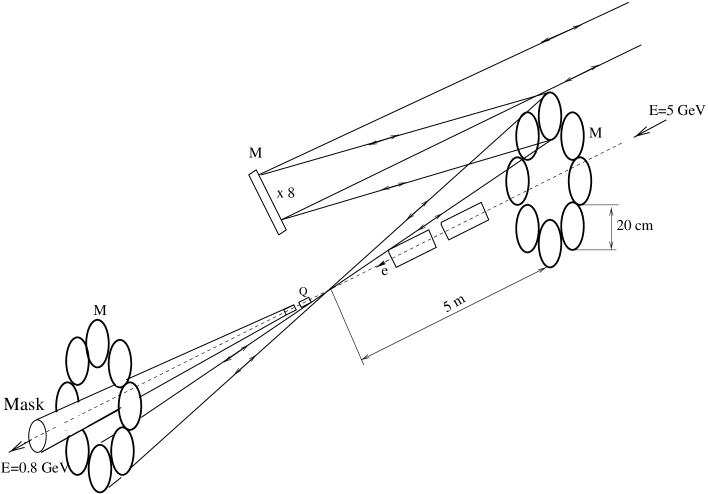
Figure 3: Possible scheme of the laser cooling.

mirrors are shown). The system consist of 8 independent identical optical cavities focusing the laser beams to the points distibuted along the beam direction on the length $\Delta z\sim 2$ mm. The length of the cavity (the distance between the “left” mirror and an entrance semi-transparent mirror (not shown)) is equal to half the distance between the electron bunches in the train, 50 m for TESLA). The large enough angle between the edges of the mirrors and the beam axis (30 mrad) makes X-ray flux rather small (see the estimation above). Also this clear angle allows the final quads to be placed at a distance about 50 cm (from the side of the cooled beam), much closer than the focusing mirrors. Smaller focal distance makes the problem of chromaticity correction easier.

The maximum distance from the CP to the mirrors is determined only by the mirror size, the diameter of 20 cm seems reasonable, which gives $L=5$ m. The laser spot size at the CP is 7.5 $\mu$m, at least 3 times larger than the horizontal electron beam size with $\beta_{x}<$ 5 mm. The circulating flash energy in each cavity is 25 J and 200 J in the whole system, not small. The average power circulating inside the system is $200\times 15$ kHz = 3 MW! However, if the Q factor of the cavities is about 1000–3000 (3000 bunches in the electron train at TESLA), the required laser power is only 1–3 kW, or 0.15–0.4 kW/per each laser, that is already reasonable.

What about damage to the mirrors by such powerful laser light? The maximum laser flash energy/cm² on the mirrors is 0.13 J/cm² (0.7-2 has been achieved for 1 ps pulses [1]), the average power/cm² is 2 kW/cm² (there are systems with $>5$ kW/cm² working long time [1]). The average power inside one train ($\Delta t=1$ msec) is 200 times higher (400 J/cm²/1 msec), but from the same ref.[1] is known that 100 J/cm² for a time of 100 ns is OK, and extrapolating as $\sqrt{t}$ (thermoconductivity) one can expect the limit of about 10 kJ for 1 msec, much larger that expected in our case. One of potential problems is the vatiation of the laser amplifire temperatute inside one beam train, that is not simple to correct by adaptive optics. Note, here we are speaking about circulating, not absorbed energy. So, all power densities are below the known limits, this all depends, of course, on specific choice of mirrors.

At last, the main numbers. After one stage of such a cooling system the normalized emittance is decreased by a factor of 6. The ultimate normalized emittance (after several cooling sections) is proportional to the $\beta$-function at the CP, at $\beta_{x,y}=1$ mm it is about $2\times 10^{-9}$ m rad, smaller than can be produced by the TESLA damping ring by a factor of 5000(15) in x(y) directions. From this point of view such a small $\beta_{x}$ is not necessary, but it should be small enough ($<5$ mm to have a small electron spot size in the cooling region. The first stage of cooling will be the most efficient because the beam is cooled in both horizontal and vertical directions (far from the limits). Besides, after decreasing the horizontal emittance the $\beta$- function at the LC final focus can be made as small as possible, $\sim\sigma_{z}.$ All together this can give a factor of ten in the luminosity.

11 Conclusion

The laser cooling of electron beams allows to reach a very luminosity at the high energy gamma-gamma colliders, 1–2 orders high than it is possible without such cooling. The method is quit straighforward, but the task is quit chelenging due to very high required laser power (peak and average). There are hopes that this problem can be solved using pulse stacking of laser pulses in an “external” optical cavity. This requires intensive R&D.

References

- [1] Zeroth-Order Design Report for the Next Linear Collider LBNL-PUB-5424, SLAC Report 474, May 1996.
- [2] Conceptual Design of a 500 GeV Electron Positron Linear Collider with Integrated X-Ray Laser Facility DESY 97-048, ECFA-97-182. R.Brinkmann et al., Nucl. Instr. &Meth. A 406 (1998) 13.
- [3] JLC Design Study, KEK-REP-97-1, April 1997. I.Watanabe et. al.,KEK Report 97-17.
- [4] I.Ginzburg, G.Kotkin, V.Serbo, V.Telnov,Pizma ZhETF, 34 (1981)514; JETP Lett. 34 (1982)491.
- [5] I.Ginzburg, G.Kotkin, V.Serbo, V.Telnov,Nucl.Instr. & Meth. 205 (1983) 47.
- [6] I.Ginzburg, G.Kotkin, S.Panfil, V.Serbo, V.Telnov, Nucl.Instr.&Meth. 219(1984)5.
- [7] V.Telnov,Nucl.Instr.&Meth.A 294 (1990)72.
- [8] V.Telnov, Nucl.Instr.&Meth.A 355(1995)3.
- [9] Proc.of Workshop on Colliders, Berkeley CA, USA, 1994, Nucl. Instr. &Meth. A 355(1995).
- [10] V.Telnov, Int. J. Mod. Phys. A 13 (1998) 2399, e-print:hep-ex/9802003.
- [11] V.Telnov, Proc. of 17th Intern. Conference on High Energy Accelerators (HEACC98), Dubna, Russia, 7-12 Sept. 1998, KEK preprint 98-163, e-print: hep-ex/9810019.
- [12] V.Telnov, Talk at International Conference on the Structure and Interactions of the Photon (Photon 99), Freiburg, Germany, 23-27 May 1999. Submitted to Nucl.Phys.Proc.Suppl.B, e-print: hep-ex/9908005
- [13] V.Telnov, To be published in the proceedings of World-Wide Study of Physics and Detectors for Future Linear Colliders (LCWS 99), Sitges, Barcelona, Spain, 28 Apr - 5 May 1999, e-print: hep-ex/9910010.
- [14] V.Telnov, Proc. of ITP Workshop “Future High energy colliders” Santa Barbara, USA, October 21-25, 1996, AIP Conf. Proc. No 397, p.259-273; e-print: physics/ 9706003.
- [15] H.Wiedemann, Particle Acc. Physics: basic principles and linear beam dinamics, Springer-Verlag, 1993.
- [16] C.Travier, Nucl.Instr.&Meth.A 340(1994)26.
- [17] V.Telnov, SLAC-PUB-7337, Phys.Rev.Lett., 78 (1997) 4757, erratum ibid 80 (1998) 2747, e-print: hep-ex/9610008.
- [18] V.Telnov, Proc. Advanced ICFA Workshop on Quantum aspects of beam physics, Monterey, USA, 4-9 Jan. 1998, World Scientific, p.173, e-print: hep-ex/9805002.
- [19] R.Palmer Nucl.Instr.&Meth.A 355(1994)150.
- [20] V.Telnov, To be published in the proceedings of World-Wide Study of Physics and Detectors for Future Linear Colliders (LCWS 99), Sitges, Barcelona, Spain, 28 Apr - 5 May 1999, e-print: hep-ex/9910011.
- [21] V.Berestetskii, E.Lifshitz and L.Pitaevskii, Quantum Electrodynamic, Pergamont press, Oxord, 1982.
- [22] G.Kotkin, S.Polityko, V.Serbo, Nucl.Instr.&Meth.A 405(1998) 30.
- [23] K. van Bibber, M.Perry, Talk at Intern. Workshop on Physics and experiments at Linear Colliders, Sitges, Spain, April 28, 1998.
- [24] V.Telnov, in Proc. of this Symposium.
- [25] T.Smith, P.Haar, H.Schwettman, Nucl. Instr. &Meth. A 393 (1997) 245 .