On the Parameterization
of the Longitudinal Hadronic Shower
Profiles in Combined Calorimetry

Abstract

The extension of the longitudinal hadronic shower profile parameterization which takes into account non-compensations of calorimeters and the algorithm of the longitudinal hadronic shower profile curve making for a combined calorimeter are suggested. The proposed algorithms can be used for data analysis from modern combined calorimeters like in the ATLAS detector at the LHC.
Keywords: Calorimetry; Computer data analysis.

One of the important questions of hadron calorimetry is the question of the longitudinal development of hadronic showers. This question is especially important for a combined calorimeter.

There is the well-known parameterization of the longitudinal hadronic shower development from the shower origin, suggested in [1]. In [2] this parameterization has been transformed to the parameterization from the calorimeter face

$$\frac{dE(x)}{dx} = N\ \Biggl{\{}\frac{wX_{0}}{a}\biggl{(}\frac{x}{X_{0}}\biggr{)}^{a}e^{-b\frac{x}{X_{0}}}{}_{1}F_{1}\biggl{(}1,a+1,\biggl{(}b-\frac{X_{0}}{\lambda_{I}}\biggr{)}\frac{x}{X_{0}}\biggr{)}$$ (1)

$$+\ \frac{(1-w)\lambda_{I}}{a}\biggl{(}\frac{x}{\lambda_{I}}\biggr{)}^{a}e^{-d\frac{x}{\lambda_{I}}}{}_{1}F_{1}\biggl{(}1,a+1,\bigl{(}d-1\bigr{)}\frac{x}{\lambda_{I}}\biggr{)}\Biggr{\}}\ ,$$

here ${}_{1}F_{1}(\alpha,\beta,z)$ is the confluent hypergeometric function, $X_{0}$ is the radiation length, $\lambda_{I}$ is the interaction length, $N$ is the normalization factor; $a$, $b$, $d$ and $w$ are parameters: $a=0.6165+0.3193\ lnE$, $b=0.2198$, $d=0.9099-0.0237\ lnE$, $w=0.4634$. Note that the formula (1) is given for a calorimeter characterizing by the certain $X_{0}$ and $\lambda_{I}$ values. At the same time, the values of $X_{0}$, $\lambda_{I}$ and the $e/h$ ratios are different for electromagnetic and hadronic compartments of a combined calorimeter. So, it is impossible straightforward use of the formula (1) for the description of a hadronic shower longitudinal profiles in combined calorimetry.

We have suggested the following algorithm of combination of the electromagnetic calorimeter ($em$) and hadronic calorimeter ($had$) curves of the differential longitudinal hadronic shower energy deposition $dE/dx$. At first, a hadronic shower develops in the electromagnetic calorimeter to the boundary value $x_{em}$ which corresponds to certain integrated measured energy $E_{em}(x_{em})$. Then, using the corresponding integrated hadronic curve, $E(x)=\int_{0}^{x}(dE/dx)dx$, the point $x_{had}$ is found from equation $E_{had}(x_{had})=E_{em}(x_{em})+E_{dm}$. Here $E_{dm}$ is the energy loss in the dead material placed between the active part of the electromagnetic and the hadronic calorimeters. From this point a shower continues to develop in the hadronic calorimeter. In principle, instead of the measured value of $E_{em}$ one can use the calculated value of $E_{em}=\int_{0}^{x_{em}}(dE/dx)dx$ obtained from the integrated electromagnetic curve. In this way, the combined curves have been obtained.

These longitudinal hadronic shower develompent curves have been compared with the experimental data obtained by the combined calorimeter consisting of the lead-liquid argon electromagnetic part and the tile iron-scintillator hadronic part [3]. This calorimeter has been exposed by the pion beams with energies of 10 – 300 GeV.

To reconstruct the hadron energy in longitudinal segments the new method of the energy reconstruction has been used [4]. In this non-parametrical method the energy of hadrons in a combined calorimeter is determined by the following formula:

$$E=1/e_{em}\cdot(e/\pi)_{em}\cdot R_{em}+1/e_{had}\cdot(e/\pi)_{had}\cdot R_{had}+E_{dm}\ ,$$ (2)

here $R_{em}$ ($R_{had}$) is the electromagnetic (hadronic) calorimeter response, $e_{em}$ ($e_{had}$) is the electron calibration constants for the electromagnetic (hadronic) calorimeter. The $(e/\pi)_{em}$ ($(e/\pi)_{had}$) ratio is

$$\Bigl{(}\frac{e}{\pi}\Bigr{)}_{cal}=\frac{(e/h)_{cal}}{1+((e/h)_{cal}-1)f_{\pi^{0},\ cal}}\ ,$$ (3)

where $cal=em,\ had$. For the electromagnetic and hadronic calorimeters the values of $(e/h)_{em}=1.7$ and $(e/h)_{had}=1.3$ are used. The fraction of the shower energy going into the electromagnetic channel for electromagnetic compartment is $f_{\pi^{0},\ em}=0.11\cdot ln{(E_{beam})}$. The electromagnetic fraction in the hadronic calorimeter is equal to the one for shower with energy $E_{had}$: $f_{\pi^{0},\ had}=0.11\cdot ln{(E_{had})}$, where $E_{had}=1/e_{had}\cdot(e/\pi)_{had}\cdot R_{had}$. This method uses only the known $e/h$ ratios and the electron calibration constants, does not require the previous determination of any parameters by a minimization technique, does not distort a longitudinal shower profile and demonstrates the correctness of the reconstruction of the mean values of energies within $\pm 1\%$. Using this energy reconstruction method, the energy depositions $E_{i}$ have been obtained in each longitudinal sampling with the thickness of $\Delta x_{i}$ in units $\lambda_{\pi}$ [3, 5].

Fig. 1 shows the differential energy depositions $(\Delta E/\Delta x)_{i}=E_{i}/\Delta x_{i}$ as a function of the longitudinal coordinate $x$ in units $\lambda_{\pi}$ for the 10 – 300 GeV and comparison with the combined curves for the longitudinal hadronic shower profiles (the dashed lines). It can be seen, there is a significant disagreement in the region of the electromagnetic calorimeter and especially at low energies.

We attempted to improve the description and to include such essential feature of a calorimeter as the $e/h$ ratio. Several modifications and adjustments of some parameters of this parameterization have been tried. It turned out that the changes of two parameters $b$ and $w$ in the formula (1) in such a way that

$$b=0.22\cdot(e/h)_{cal}/(e/h)_{cal}^{\prime}\ ,$$ (4)

$$w=0.6\cdot(e/\pi)_{cal}/(e/\pi)_{cal}^{\prime}$$ (5)

made it possible to obtain the reasonable description of the experimental data. Here the values of the $(e/h)_{cal}^{\prime}$ ratios are $(e/h)^{\prime}_{em}\approx 1.1$ and $(e/h)^{\prime}_{had}\approx 1.3$ which correspond to the data used for the Bock parameterization [1]. The $(e/\pi)_{cal}^{\prime}$ are calculated using formula (3).

In Fig. 1 the experimental differential longitudinal energy depositions and the results of the description by the extension of the parameterization (the solid lines) are compared. There is a reasonable agreement (probability of description is more than 5%) between the experimental data and the curves, taking into account uncertainties in the parameterization function.

So, we propose the extension of the longitudinal hadronic shower profile parameterization which takes into account non-compensations of calorimeters and the algorithm of the longitudinal hadronic shower profile curve making for a combined calorimeter.

We are thankful Peter Jenni, Marzio Nessi and Julian Budagov for fruitful discussions and support of this work.

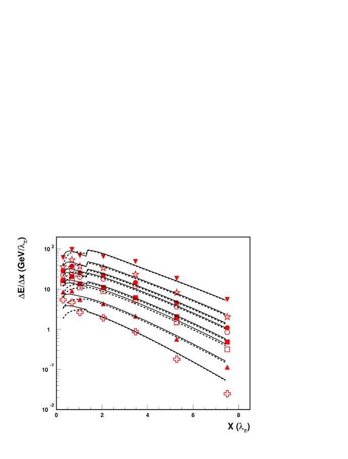
Figure 1: The experimental differential longitudinal energy depositions at 10 GeV (crosses), 20 GeV (black top triangles), 40 GeV (squares), 50 GeV (black squares), 80 GeV (circles), 100 GeV (black circles), 150 GeV (stars), 300 GeV (black bottom triangles) energies as a function of the longitudinal coordinate $x$ in units $\lambda_{\pi}$ for the combined calorimeter and the results of the description by the Bock et al. (dashed lines) and modified (solid lines) parameterizations.

References

- [1] R. Bock et al., Nucl. Instr. and Meth. 186 (1981) 533.
- [2] Y.A. Kulchitsky, V.B. Vinogradov, Nucl. Instr. and Meth. A413 (1998) 484.
-
[3]
ATLAS Collaboration,
Results from a new combined test of an electromagnetic liquid-argon
calorimeter with a hadronic scintillating-tile calorimeter,
Submitted to Nucl. Instr. and Meth. A, 1999.
M. Cobal et al., ATL-TILECAL-98-168, CERN, Geneva, Switzerland. - [4] Y.A. Kulchitsky et al., JINR-E1-99-317, JINR, Dubna, Russia, 1999.
- [5] Y.A. Kulchitsky et al., JINR-E1-99-326, JINR, Dubna, Russia, 1999.