[

Chaos and Universality in the Dynamics of Inflationary Cosmologies

Abstract

We describe a new statistical pattern in the chaotic dynamics of closed inflationary cosmologies, associated with the partition of the Hamiltonian into rotational motion energy and hyperbolic motion energy pieces, in a linear neighborhood of the saddle-center present in the phase space of the models. The hyperbolic energy of orbits visiting a neighborhood of the saddle-center has a random distribution with respect to the ensemble of initial conditions, but the associated histograms define a statistical distribution law of the form $p(x)=C\,x^{-\gamma}$, for almost the whole range of hyperbolic energies considered. We present numerical evidence that $\gamma$ determines the dimension of the fractal basin boundaries in the ensemble of initial conditions. This distribution is universal in the sense that it does not depend on the parameters of the models and is scale invariant. We discuss possible physical consequences of this universality for the physics of inflation.

]

The general dynamics of closed Friedmann-Robertson-Walker (FRW) inflationary cosmologies, with a minimally coupled massive scalar field and perfect fluid or with anisotropy, is chaotic[1, 2]. The chaotic behaviour has a definite homoclinic origin, due to infinite transversal crossings of homoclinic cylinders present in the phase space of the models, analogous to the case of breaking and crossing of homoclinic connections in Poincaré’s homoclinic phenomena[3, 4, 5, 6, 7]. The topology of homoclinic cylinders is a consequence of a critical point of the saddle-center type[6] in phase space, and the breaking and crossings of the cylinders are due to the non-integrability of the dynamics. These homoclinic phenomena produce chaotic sets in phase space, in the sense that the dynamics is highly sensitive to fluctuations in initial conditions taken on these sets. The aim of this communication is to describe a new statistical pattern in the chaotic dynamics engendered by the saddle center and what are its possible consequences in the physics of inflation. Throughout the paper we use units such that $8\,\pi\,G=1=c$.

Our discussion will be basically restricted to closed Friedmann-Robertson-Walker (FRW) inflationary cosmologies, with a minimally coupled massive scalar field and perfect fluid, but the same construction will apply to a Bianchi IX anisotropic cosmology and yields analogous results, as we will see. The equations of motion may be derived from the Hamiltonian constraint

$$H=-\frac{p_{\varphi}^{2}}{2\,a^{2}}+\frac{p_{a}^{2}}{12}+3\,a^{2}-a^{4}\,V(\varphi)-E_{0}=0,$$ (1)

where $a$ and $\varphi$ are the scale factor and the scalar field, respectively, and $p_{a}$ and $p_{\varphi}$ are the momenta canonically conjugate to $a$ and $\varphi$. We consider here a perfect fluid describing radiation, and the potential $V(\varphi)=\Lambda+\frac{1}{2}\,m^{2}\,\varphi^{2}$. The constant $\Lambda$ is considered to correspond to the vacuum energy of the scalar field $\varphi$, and plays the role of a cosmological constant term. This model may be thought to describe a classical universe just exiting a Planck era. $E_{0}$ is a constant arising from the first integral of the Bianchi identities, and proportional to the total matter energy of the models. The dynamical system generated by (1) has a saddle-center critical point in the finite region of the phase space with coordinates $E:\varphi=0,a=a_{0}=\sqrt{\frac{3}{2\,\Lambda}},p_{a}=0,p_{\varphi}=0$. The energy associated to the critical point $E$ is $E_{0}=E_{crit}=\frac{3\,a_{0}^{2}}{2}$. The phase space also has a pair of critical points at infinity, corresponding to the DeSitter solution, one acting as an attractor, and the other as a repeller; the DeSitter attractor characterizes an exit to inflation for the models.

In accord to a theorem by Moser[8], it is always possible to find a set of canonical variables such that, in a linear neighborhood of a saddle-center, the Hamiltonian dynamics is separable into rotational motion and hyperbolic motion pieces, with the associated partial energies $E_{rot}$ and $E_{hyp}$ approximately conserved. The canonical variables $(a,\varphi,p_{a},p_{\varphi})$ behave as Moser’s variables in a small neighborhood of $E$; in fact, expanding the Hamiltonian (1) about $E$ we obtain

$$H=E_{hyp}-E_{rot}+(E_{cr}-E_{0})+{\cal{O}}(3)=0,$$ (2)

where $E_{rot}=\frac{1}{2}\,\frac{p_{\varphi}^{2}}{a_{0}^{2}}+\frac{1}{2}\,m^{2}\,a_{0}^{4}\,\delta\,\varphi^{2}$ and $E_{hyp}=\frac{1}{12}\,p_{a}^{2}-6\,\delta\,a^{2}$, with $\delta\,a=a-a_{0}$, $\delta\,\varphi=\varphi$, and $(E_{cr}-E_{0})$ small. ${\cal{O}}(3)$ denotes higher order terms which are neglected in a small neighborhood of $E$. In this approximation the scale factor $a(t)$ has pure hyperbolic motion, and is completely decoupled from the scalar field pure rotational motion in the plane $(\varphi,p_{\varphi})$.

We will now focus our attention to chaotic aspects in the dynamics, leading us into a statistical treatment of possible experiments made in the models. Our description will be restricted to sets of orbits which visit a linear neighborhood of the saddle-center $E$, and makes extensive use of the partition of energy $E_{hyp}-E_{rot}+(E_{crit}-E_{0})\approx 0$ that occurs in this neighborhood. Let us consider a set ${\cal{D}}$ of arbitrary initial conditions which correspond to initially expanding universes with energy $E_{0}$, and such that all the orbits visit a linear neighborhood of $E$. The set ${\cal{D}}$ may be represented as a small 4-dim volume, contained in a 4-dim sphere of radius $R$ (of order $10^{-5}$, $10^{-6}$, …, depending on the order of fluctuations we admit in the initial conditions) constructed about the point, say, $(0.4,0,3.5638181771,0)$ in phase space, and satisfying the Hamiltonian constraint (1). The above point belongs to the invariant plane $p_{\varphi}=\varphi=0$, and is located on one of the separatrices reaching the saddle-center $E$. We denote $R$ as the characteristic radius of the four volume ${\cal{D}}$. One of the chaotic aspects we single out for this set is the definition of a chaotic exit to inflation[1, 2], connected to the existence of fractal basin boundaries in the set ${\cal{D}}$. For a given radius $R$ of ${\cal{D}}$, it is always possible to find a gap of energy $\delta\,E^{*}$ (which depends on $R^{2}$) such that for $E_{0}\in\delta\,E^{*}$, the exit to inflation is chaotic, namely, small fluctuations (of order of, or smaller than $R$) of the initial conditions will change the asymptotic state of the orbits from collapse into escape to inflation, and vice versa, after visiting the neighborhood of the saddle-center. The chaotic exit to inflation may be characterized in terms of the partition of energy (2): for a particular orbit, the partition into the approximately conserved energies $E_{hyp}$ and $E_{rot}$ about the critical point will determine the asymptotic state of the orbit, namely, collapse or escape to inflation, whether respectively $E_{hyp}<0$ or $E_{hyp}>0$. However, we are no longer able to foretell precisely what will be the value of $E_{hyp}$ endowed to a given orbit of ${\cal{D}}$ when it visits a neighborhood of $E$, due to the high sensitivity of $E_{hyp}$ with the fluctuations of the initial conditions, a consequence of the chaotic nature of the set ${\cal{D}}$. In what follows, we will use standard statistical methods to examine this instability of the partition of the energy, a procedure which will lead us into the recognition of new statistical patterns for chaotic sets in the phase space.

To start, let us make a plot of $E_{hyp}$ versus the ordered values of one of the canonical variables, say $a$, especifying the initial conditions in the set ${\cal{D}}$, for $R\approx 10^{-5}$, $m=2$ and $(E_{crit}-E_{0})=10^{-10}$. We fixed the value of $\Lambda=3/2$, such that $a_{0}=1$ and $E_{crit}=3/2$. Fig. 1 corresponds to $3,031$ initial conditions, sampled randomly and uniformly in ${\cal{D}}$, and the points were connected for successive a’s to a better visualization. The result shows a highly disorganized ”signal”, displaying structures in all scales of $a$. Analogous highly disorganized ”signals” appears for other variables $\varphi$, $p_{a}$, or $p_{\varphi}$. Also, if another sample of points is taken randomly and uniformly in ${\cal{D}}$, we obtain a ”signal” with the same general aspect but completely different in all the details, appearing not to have any connection with the previous figure. However a pattern of the signal is reproducible, which is its histogram.

Our basic procedure is to realize the following numerical experiments with the system: from a given ensemble ${\cal{D}}$ of initial conditions, we generate orbits of the system by the full Hamiltonian dynamical equations derived from (1). These orbits visit a linear neighborhood of the saddle-center $E$. In this linear neighborhood, we calculate the approximately conserved quantity $E_{hyp}$ associated with each orbit ; for practical purposes, $E_{hyp}$ is evaluated at the point of closest approach to $E$, in the sense of the Euclidean measure. We construct the histogram function $P_{E_{hyp}}=\Delta\,N(E_{hyp})/\Delta\,E_{hyp}$ as usual: the $E_{hyp}$ axis is divided into a large number of equal small bins $\Delta\,E_{hyp}$ and the histogram is given by the number of orbits assigned with hyperbolic energy in the interval $[E^{(i)}_{hyp}-\Delta\,E_{hyp}/2,E^{(i)}_{hyp}+\Delta\,E_{hyp}/2]$ , when the orbit visits the neighborhood of $E$. Here $E^{(i)}_{hyp}$ is the value of the hyperbolic energy centered in the $i$-th bin. We fix the origin of the histogram in $E^{min}_{hyp}$, which is the minimum value of $E_{hyp}$ obtained in the numerical experiment; according to (2), $E^{min}_{hyp}\geq-(E_{crit}-E_{0})$. We also note that due to (2) the histogram of the signal associated with $E_{rot}$ results merely from a shift of the histogram for $E_{hyp}$.

A careful examination shows us that the form of the histogram for smaller values of $E_{hyp}$ is sensitive to the geometry of the sampling set ${\cal{D}}$. We must therefore establish a criterion to fix the geometry of ${\cal{D}}$ such that no bias due to the geometry of the sampling volume manifests itself in the histogram, and such that the statistical distribution function obtained from the histogram will be connected only to the non-integrability of the system. We establish that the domain ${\cal{D}}$ of randomly and uniformly distributed phase space points must have a geometry such that it yields histograms $\Delta\,N(E_{hyp})/\Delta\,E_{hyp}$ or $\Delta\,N(E_{rot})/\Delta\,E_{rot}$ for the integrable Hamiltonian $H=\frac{1}{2}\,(p_{\varphi}^{2}+m^{2}\,\varphi^{2})+\frac{1}{12}\,p_{a}^{2}-6\,a^{2}$ having the form of a plateau (cf. also the caption of Figs. 2). In the case of the non-integrable Hamiltonian (1) the histogram constructed from the same set of initial conditions ${\cal{D}}$ deviates from a plateau, reflecting the nonintegrability of the system. Figs. 2(a,b) show $30,000$ initial conditions sampled randomly and uniformly in ${\cal{D}}$ constructed for $m=10$, $R\approx 10^{-5}$ and $(E_{crit}-E_{0})=10^{-10}$, projected on the planes $(\varphi,p_{\varphi})$ and $(a,p_{a})$. Fig. 3 shows the histogram generated from the initial conditions set ${\cal{D}}$ of Fig. 2 by the non-integrable Hamiltonian (1).

At this point our main question is: what are the possible candidates for the statistical energy distribution law associated with the histogram function? The present histograms have an excess in the tails, namely, in the region of large positive hyperbolic energies, relative to the corresponding Maxwell-Boltzmann distribution. Indeed, a trivial log-linear plot of the histogram shows a non linear form for the tails, exhibiting an anomalous behaviour in contrast to the case of the normal Maxwell-Boltzmann distribution. This is not surprizing since we are dealing with a system were long range interactions are present, and where relevant phase-space sets are chaotic and have a fractal-like structure. The system is certainly not in the realm of Boltzmann-Gibbs statistical mechanics, which essentially focus on non-interacting or short-range interacting many-body Hamiltonian systems. After extensive numerical analysis, we obtained that all histograms examined are fitted by the energy distribution function

$$P(x)=C_{0}\,\beta\,(\beta\,x)^{-\gamma},$$ (3)

where $C_{0}$ is an adimensional normalization constant and $x=(E_{hyp}-E^{min}_{hyp})$. The parameters of the distribution have values $\gamma=0.6354\pm 0.02527$, $C_{0}\,\beta^{1-\gamma}\,\times\,10^{10\,\gamma}=12.496\pm 0.5108$. These are the values for the best fit of the histogram of Fig. 3, with the square of the variance $\chi^{2}=0.06022$, obtained using the PAW packet from CERN. Within statistical errors, the value $\gamma\cong 0.6354$ corresponds to the best fit of all histograms generated with the dynamics of (1). For comparison purposes, all histograms were normalized by fixing the peak with the value $100$.

The distribution law (3) produces an accurate fit for almost the whole range of energies of the histograms. The continuous line in Fig. 3 shows the best fit of (3) to the histogram. The whole histogram is composed of $100$ bins, each with $\Delta\,E_{hyp}=7.33993555\times 10^{-12}$. To obtain the fit with the value $\chi^{2}=0.06022$, we have neglected the extreme of the tail of the histogram, more specifically from the $55^{th}$ bin on. If we have extended the solid curve beyond this bin, a discrepancy between the curve and the histogram would appear. This discrepancy at the end of the tail has the following explanation. The cut-off at the largest values of $E_{hyp}$ is due to the finite volume of the sampling set ${\cal{D}}$. If we increase $R$ (consequently increasing the volume) and maintain the same uniform density of points, the cut-off is shifted to the right and the tail of the histogram raises improving the fit in this region. The left extremity is a peak. If we extended (3) to values of $x$ very close to zero, the peak might suggest a divergence in the density of states - a property which is not physically reasonable for statistical ensembles - but this is not the case. Indeed the smallest values of $E_{hyp}$ in our histograms are associated to points that are located at the boundaries in $(a,p_{a})$ of the linear neighborhood of the saddle-center $E$, and the evidence from the histograms is that, as we increase the volume of ${\cal{D}}$, there is a saturation in the corresponding increase of the peak of the histograms. Therefore the distribution function (3) must surely be corrected, to be finite in the neighborhood of $x=0$. The saturation is possibly due to the fact that, as we enlarge the volume, we approach the limit of validity of the linear approximation, and higher order terms in the Hamiltonian may be contributing already to make the density of states finite there. The parameter $\gamma$ is adimensional while $1/\beta$ must have the dimension of energy. We may tentatively interpret the latter as defining a temperature for the saddle-center. For the integrable case, $\gamma=0$.

The following characterist properties of the histograms were verified numerically, through exhaustive numerical experiments realized with randomly and uniformly distributed distinct sampling sets ${\cal{D}}$ having the same geometry described in Figs. 2:

$(i)$ the form of the histogram is scale invariant, that is, it is independent of the characteristic radius $R$ of the sampling set ${\cal{D}}$ of initial conditions, modulo a change of bin;

$(ii)$ the form of the histogram is independent of the parameter $(E_{crit}-E_{0})$ that allows to characterize if the orbits are dominantly collapsing or escaping, after visiting the neighborhood of the saddle-center $E$;

$(iii)$ the form of the histogram is independent of the mass parameter $m$;

$(iv)$ the histogram has the same form also for a model with dust, what lead us to conjecture its independence of the particular equation of state $p=\lambda\,\rho$, with $0\leq\lambda\leq 1$;

$(v)$ within statistical errors, the value $\gamma\cong 0.6354$ corresponds to the best fit of all histograms associated with the Hamiltonian (1).

We were not able to identify (3) with any known statistical distribution. However, we are aware that this behaviour is typical of tails of distributions arising in Tsallis generalized statistics[9], that were proposed in order to accomodate, at least in part, systems which have an anomalous behaviour with respect to Boltzmann-Gibbs statistics.

We now exhibit numerical evidence that the constant $\gamma$ appearing in (3) may characterize the fractal nature of the sets ${\cal{D}}$, more specifically, it may give a measure of the fractal dimension of basin boundaries in these sets. In fact, by using a box counting method[10] with the uncertainty code defined by collapse/escape, we obtained the uncertainty exponent $\alpha\cong 0.36931$ for the set ${\cal{D}}$ with $m=10$, $(E_{crit}-E_{0})=10^{-10}$ and $R=10^{-5}$ (cf. Fig. 5). Within statistical errors, this same value was obtained for all initial conditions sets with $E_{0}\in\delta\,E^{*}$, used to construct histograms in our numerical experiments, implying that

$$\gamma+\alpha\approx 1.$$ (4)

As a consequence $\gamma$ appears to be directly related to the fractal dimension $d$ of the basin boundaries of ${\cal{D}}$, since in our boxcounting calculation $d=N-\alpha$, where $N=3$ is the dimensionality of ${\cal{D}}$. The above restriction to sets ${\cal{D}}$ with $E_{0}\in\delta\,E*$ is due to the fact that in these sets we may define the uncertainty code collapse/escape; for sets with $E_{0}\notin\delta\,E^{*}$, other uncertainty code may be used.

We have also examined the Hamiltonian

$$H = \frac{1}{4\,B}\,P_{A}\,P_{B}-\frac{1}{8\,B^{2}}\,A\,P_{A}^{2}+2\,A-\frac{1}{2}A^{3}\,B^{2}-$$ (6)

$$2\,\Lambda\,B^{2}-E_{0}=0,$$

describing the dynamics of anisotropic spatially homogeneous Bianchi IX cosmological models, with scale factors $A$ and $B$, plus a cosmological constant and a perfect fluid in the form of dust. This system is chaotic and has a saddle-center in the finite region of phase space[2]. We made the same construction of histograms for hyperbolic/rotational energies in a linear neighborhood of the saddle-center; in this case, we have the burden of obtaining Moser’s normal coordinates in order to calculate properly the hyperbolic/rotational energies associated to each orbit when visiting the neighborhood of the saddle-center. Fig. 4 shows the histogram generated from 30,000 initial conditions. The geometry of the initial conditions set satisfies the same criteria of the previous case (1). The continuous line corresponds to the best fit of (3), with $\gamma=0.71458\pm 0.04060$, $C_{0}\,\beta^{1-\gamma}\times 10^{10\gamma}=11.601\pm 0.7711$, and $\chi^{2}=0.06685$. The histograms consists of 65 bins, each with value $\Delta\,E_{hyp}=3.58919436\times 10^{-12}$. The best fit was realized in the interval of the $2^{nd}$ to the $30^{th}$ bin. Within statistical errors, all histograms associated with (5) are fitted by the distribution function (3) with $\gamma\cong 0.714$. Properties $(i)$ and $(ii)$ were also verified for the present case. A boxcounting for the initial conditions set yields the uncertainty exponent $\alpha\cong 0.28103$, confirming the relation $\gamma+\alpha\cong 1$.

We end this paper by making the conjecture that the statistical distribution (3) is an universal characteristic of saddle-center critical points, independent of the particular dynamical system in consideration. We are presently working in this direction by making the same constructo for two other Hamiltonian systems presenting a saddle-center in their phase space, not in the realm of inflationary cosmologies: the Hénon-Heiles system[11] and the chemical system examined in Ref. [12]. Our preliminary results indicate the same distribution function (3) with distinct values of $\gamma$ for each system. We also conjecture whether other critical points of different nature can be universally characterized in this way.

The above results may have some interesting physical applications for the dynamics of preinflationary models immediately before the universe enters the inflationary regime or recollapses, both alternatives depending on the typical fluctuations in the system. For instance, we may use the statistical function (3) to calculate the average value of the hyperbolic energy for ensembles of universes. As we know[1, 2] the sign of this average hyperbolic energy determines the ”average” long time behaviour of the ensemble, that is, collapse or escape to inflation. A straightforward calculation shows that the sign of the average energy depends basically on $((1-\gamma)\,\beta\,E^{max}_{hyp}+\beta\,E^{min}_{hyp})$, where $E^{max}_{hyp}$ is the maximum value of the hyperbolic energy in the histogram. The relative value of $E^{min}_{hyp}$ decreases linearly (and may exceed in absolute value $E^{max}_{hyp}$) with the increase of $(E_{crit}-E_{0})$, implying that larger/smaller values of $(E_{crit}-E_{0})$ determine the dominance of collapse/escape in the dynamics of the ensemble ${\cal{D}}$ of universes.

The authors are grateful to Prof. C. Tsallis for stimulating discussions concerning the generalized statistics. We are also indebted to the graduate students of LAFEX/CBPF, for introducing us to the use of PAW. Financial support from CNPQ and FAPERJ is acknowledged. H. P. de Oliveira is grateful to the International Center of Theoretical Physics (ICTP) for support.

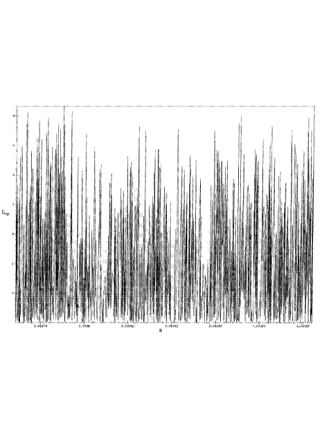
FIG. 1.: Signal resulting from the distribution of hyperbolic energies $E_{hyp}$ versus the ordered initial values of $a$. We considered 1,035 initial conditions sampled randomly and uniformly. Points were connected for successive $a$’s, for better visualization.

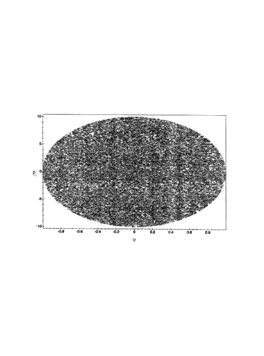
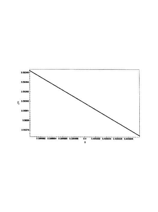
FIG. 2.: Set ${\cal{D}}$ of 30,000 initial conditions, uniformly and randomly distributed, for the case $m=10$, $E_{crit}-E_{0}=10^{-10}$ and $R=10^{-5}$, projected in the planes $\varphi,p_{\varphi}$ (Fig. 2a) and $(a,p_{a})(Fig.2b)$. The particular geometry taken for the initial conditions set is such that $(i)$ it satisfies the Hamiltonian constraint (1) and, $(ii)$ the associated histograms for the integrable case have a form of a plateau; this demands that Fig. 2a be an ellipse with axes having the ratio $m$.

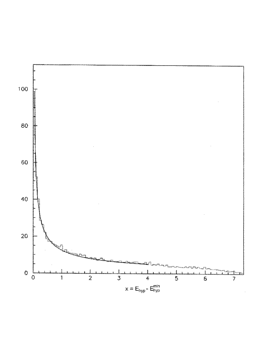
FIG. 3.: Histogram of the distribution of $E_{hyp}$, associated with the 30,000 initial conditions of Fig. 2. The continuous line is the best fit of the distribution (3) with $\gamma=0.6354\pm 0.02527$, $C_{0}\,\beta^{1-\gamma}\times 10^{10\gamma}=12.496\pm 0.5108$ and $\chi^{2}=0.06022$. The horizontal axis is scaled with the factor $10^{-10}$.

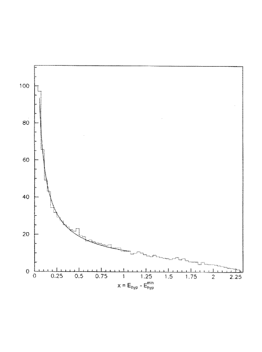
FIG. 4.: Histogram of the distribution of $E_{hyp}$, generated from 30,000 initial conditions for the anisotropic case, with $\Lambda=1/4$, $E_{crit}-E_{0}=0.5\times 10^{-10}$ and $R=10^{-5}$. The continuous line is the best fit of (3) with $\gamma=0.7146\pm 0.0406$, $C_{0}\,\beta^{1-\gamma}\times 10^{10\gamma}=11.601\pm 0.7711$ and $\chi^{2}=0.06685$. The horizontal axis is scaled with the factor $10^{-10}$.

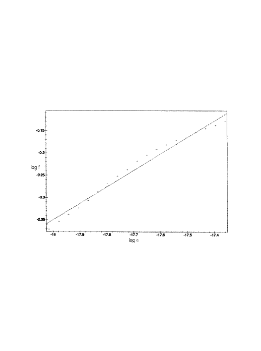
FIG. 5.: Plot of $f=k_{0}\,\epsilon^{\alpha}$ in a log-log scale, where $\epsilon$ is the uncertainty radius about 20,000 initial conditions taken inside the set ${\cal{D}}$, and $f$ is the fraction of ${\cal{D}}$ of uncertain initial conditions with the uncertainty code collapse/escape. We considered 20 values of $\epsilon$ inside the interval $[0.9\times 10^{-8},1.8\times 10^{-8}]$. The best fit renders $\alpha\approx 0.36931$.

REFERENCES

- [1] G. A. Monerat, H. P. de Oliveira and I. Damião Soares, Phys. Rev. D58, 063504 (1998).
- [2] H. P. Oliveira, I. Damião Soares and T. J. Stuchi, Phys. Rev. D56, 730 (1997).
- [3] S. Wiggins, Global Bifurcations and Chaos, Springer-Verlag, Berlin (1988).
- [4] W. M. Vieira and A. M. Osório de Almeida, Physica D 90, 9 (1996).
- [5] R. L. Devaney, J. Diff. Eq. 21, 431 (1976); A. Mielke P. Holmes and O. O’Reilly, J. Dynamics and Diff. Eqs., 4, 95 (1997).
- [6] J. Guckenheimer and P. Holmes, Dynamical Systems and Bifurcations of Vector Fields, Appl. Math. Sciences, Vol.42, Springer-Verlag, New York (1983); J. Koiller, J. R. T.de Mello Neto and I. Damião Soares, Phys.Lett. 110A, 260 (1985).
- [7] J. Moser, Stable and Random Motions in Dynamical Systems, Princeton University Press, Princeton (1973).
- [8] J. Moser, Comm. on Pure and Appl. Math. 11, 257 (1958).
- [9] C.Tsallis, J. Stat. Phys. 52, 479 (1988); E. M. F. Curado and C. Tsallis, J. Phys. A 24, L69 (1991); Corrigenda: 24, 3187 1991 and 25, 1019 (1992).
- [10] S. Blehar, C. Grebogi, E. Ott and R. Brown, Phys. Rev. A38, 930 (1988); E. Ott, Chaos in Dynamical Systems (Cambridge University Press, 1993).
- [11] M. Hénon and C. Heiles, Astron. J., 69, 73 (1964).
- [12] A. M. Osório de Almeida, N. de Leon, M. A. Metha and C. C. Marston, Physica D46, 265 (1990).