Fractals and Scars on a Compact Octagon

Abstract

A finite universe naturally supports chaotic classical motion. An ordered fractal emerges from the chaotic dynamics which we characterize in full for a compact 2-dimensional octagon. In the classical to quantum transition, the underlying fractal can persist in the form of scars, ridges of enhanced amplitude in the semiclassical wave function. Although the scarring is weak on the octagon, we suggest possible subtle implications of fractals and scars in a finite universe.

05.45.-a,05.45.Df,05.45.Mt,98.80.Cq

\begin{picture}(0.0,0.0)\put(410.0,190.0){{ }} \end{picture}

Chaos is often avoided in fundamental physics and cosmology. A recent surge of interest in a finite universe has highlighted a well known chaotic system, a compact negatively curved space [1]. Most efforts in cosmology have struggled to circumvent the inherent chaos. Instead of avoiding chaos, we investigate the structure of the chaotic flows on a compact space. Since we are able to deduce analytically many of the chaotic properties, we concentrate on the compact 2d octagon and study the classical motion and the emergent fractal properties. Poincaré realized that the periodic orbits, though seemingly special, define the entire structure of a dynamical system. With the advent of chaos, periodic orbits grow exponentially in number as a function of their length. The invariant set of periodic trajectories packs itself into a fractal to accommodate the dense proliferation of orbits. We derive a very precise counting of the periodic orbits, determine the topological entropy, derive a recurrence relation for all of the fixed points, and analytically compute a spectrum of fractal dimensions. We then numerically confirm our analytic results by generating the fixed points and measuring the dimensions of the set.

The fractals may not be effaced in the classical to quantum transition. A phenomenon known as scarring of the quantum wave function has been witnessed in systems which are classically chaotic [2]. The scars refer to ridges along which the amplitude of the semiclassical wave function is enhanced. We argue that the scars can be interpreted as the smooth remnant of the underlying classical fractal. We relate the closed orbits on the 2d space to the occurrence of scars. The compact octagon is so thoroughly chaotically mixed that the scarring is minimal, consistent with the fractal properties as discussed. In a finite model of the universe, the faint scars could seed a weblike distribution of matter threaded around the space.

Geodesic motion on a compact $2d$ pseudosphere is completely chaotic. On the Poincaré unit disc the metric can be written

$$ds^{2}=-d\eta^{2}+{4(1-r^{2})^{-2}}\left(dr^{2}+r^{2}d\phi^{2}\right).$$ (1)

Geodesics are semi-circles which are orthogonal to the boundary at $r=1$. We consider null geodesics for which the coordinates $(r,\phi)$ have the conjugate momenta

$$(\Pi_{r},\Pi_{\phi})={4(1-r^{2})^{-2}}(\dot{r},r^{2}\dot{\phi}).$$ (2)

There are two conserved quantities. Since $\dot{\Pi}_{\phi}=0$, there is a conserved angular momentum

$$L={4(1-r^{2})^{-2}}r^{2}\dot{\phi}$$ (3)

and the kinetic energy is conserved

$${1\over 2}\left(\dot{r}^{2}+r^{2}\dot{\phi}^{2}\right){4(1-r^{2})^{-2}}={1\over 2}.$$ (4)

Condition (4) is the same as the restriction that photons travel at unit speed.

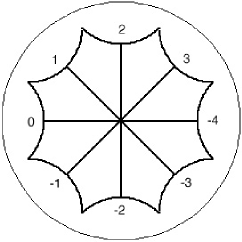
FIG. 1.: The symmetric octagon drawn in the Poincaré unit disc. The octagon forms a two-handled surface when the opposite sides are glued together. Each edge corresponds to a generator $g_{j}$ with $j=-4,..,3$ and are numbered accordingly.

We consider the simplest compact surface of negative curvature with genus 2. The fundamental domain is a symmetric regular octagon with the opposite edges identified in pairs as in fig. 1. The identifications are effected by a discrete subgroup of the Lorentz group. The horizontal identifying boost can be represented in coordinates $x=r\cos\phi$ and $y=r\sin\phi$ as

$$g_{0}=\pmatrix{\cosh\tau_{1}/2&\sinh\tau_{1}/2\cr\sinh\tau_{1}/2&\cosh\tau_{1}/2}$$ (5)

with $\cosh\tau_{1}/2=1+\sqrt{2}$, while the other four are related by a rotation of $g_{0}$ through the angle $j\pi/4$. The four generators are related to their respective inverses by a rotation through $\pi$. We denote all the generators and their inverses compactly as $g_{j}$ with $j=-4,..,3$ so that the $g_{0}g_{-4}=g_{3}g_{-1}=g_{2}g_{-2}=g_{1}g_{-3}={\bf I}$. These generators obey the one relation

$$g_{0}g_{-3}g_{2}g_{-1}g_{-4}g_{1}g_{-2}g_{3}={\bf I}.$$ (6)

FIG. 2.: The action of the map on the exit-entry domains for geodesics. An orbit is completely specified by the angular momentum $L$ and the angular coordinate $\phi(t=0)=\theta$ at which the geodesics intersects the boundary in the past. All the orbits within the darkened exit domain above exit edge 0 of fig. 1. The map takes this exit domain into the darkened vertical entry domain.

A geodesic is uniquely specified by two parameters $(\theta,L)$ where $\theta$ is the angular coordinate of the geodesic as it intersects the boundary in the past. Balasz and Voros [3] developed a reentry map which takes initial values for $(\theta,L)$ through the appropriate edge and back into the fundamental domain. The map which iterates all values through edge 0 of fig. 1 is

$$\tan(\theta_{n+1}/2) = e^{-\tau_{1}}\tan(\theta_{n}/2)$$ (7)

$$L_{n+1}=(\cosh\tau_{1} + \cos\theta_{n}\sinh\tau_{1})L_{n}-\sinh\tau_{1}\sin\theta_{n}.$$ (8)

The reentry map for orbits exiting any of the $8$ edges is effected by shifting $\theta\rightarrow\theta+j\pi/4$ for $j=-4,...3$. The map is Hamiltonian and area preserving.

A trajectory is a point in the plane $(\theta,L)$ and those trajectories lying within the intersection of the two darkened separating curves of fig. 2 exit edge 0. A separating curve is

$$L_{0}={\sin(\theta-\pi/8)\over\cos(\theta-\pi/8)-\coth\tau_{2}}$$ (9)

with $\coth\tau_{2}=2^{-5/4}(1+\sqrt{2})$. The other $7$ exit domains are shifted by $\pi/4$ as represented in fig. 2. All eight curves, $L_{j}$, are obtained from eqn. (9) by shifting $\theta\rightarrow\theta+j\pi/4$ with $j=-4,..0,..3$. The map acts very much like an eightfold Baker’s map. The $8$ sections exit their respective edges and reenter as the equal-area, nearly-vertical strips. Each of the $8$ exit strips overlaps with only $7$ of the reentry strips. In other words, the points can reenter any of the other edges except the one just exited. The original area is chopped into $8\times 7$ smaller areas, each of which continues to flow through the space and gets resegmented into $8\times 7\times 7$ new areas. The total number of pieces at order $n$ is then $8\times 7^{n-1}$. Covering the area with boxes of size $\epsilon=(1/7)^{n/2}$ gives the box-counting dimension $D_{0}=\lim_{n\rightarrow\infty}\ln(7^{n-1})/\ln(7^{n/2})=2$. The fractal fills the allowed area.

The number of periodic orbits is slightly smaller than the number of areas. The $g_{j}$ construct a symbolic alphabet out of which to build $n$-letter words. Each repeated word corresponds to a periodic orbit. The number of words of order $n$, $N(n)$, is the sum of the number of words which begin and end on the same letter, $O(n)$, and the number of words which begin and end on different letters, $\Delta(n)$,

$$N(n)=O(n)+\Delta(n).$$ (10)

A word cannot begin and end on inverse letters: a repeated $n$-letter word of the form ${g_{i}g_{j}...g_{k}g^{-1}_{i}}$ is equivalent to the repeated $(n-1)$-letter word ${g_{j}...g_{k}}$. An $n$-letter word can be built from every $O(n-1)$ by attaching any of the letters in the alphabet except the one which is inverse to the end letter. So, there are $7O(n-1)$ of these. More $n$-letter words can be built from every $\Delta(n-1)$ by attaching any of the letters in the alphabet except for the two letters which are either the inverse of the end letter or the inverse of the beginning letter. So, there are $6\Delta(n-1)$ of these. Although $(n-1)$-letter words of the form $g_{i}....g^{-1}_{i}$ do not contribute to $N(n-1)$, they do contribute to $N(n)$ (for $n\geq 3$) by adding any letter other than $g_{i}$ or $g^{-1}_{i}$. The number of words of order $(n-1)$ that begin and end on inverse letters is

$$I(n-1)=\sum_{m=2}^{m=n-2}\Delta(m).$$ (11)

It follows that

$$N(n)=7O(n-1)+6\Delta(n-1)+6I(n-1).$$ (12)

Eqn. (12) can be simplified by noting that $O(n)=N(n-1)$. We can combine these relations to reexpress (12) for $n\geq 3$ as

$$N(n)=7N(n-2)+6N(n-1)-6N(1).$$ (13)

There is additional pruning at higher orders due to the one relation eqn. (6). However, this pruning is extremely sparse and affects the counting very little. The number in (13) is actually slightly smaller than $N(n)=7^{n}$ but tends toward this behaviour as $n\rightarrow\infty$. To see this, let $N\sim b^{n}$ in the limit of large $n$ and solve for $b$ to obtain $N\rightarrow 7^{n}$. The topological entropy is then, $H_{T}=\lim_{n\rightarrow\infty}(1/n)\ln N=\ln 7$.

There is a spectrum of weighted dimensions which measures the distribution of frequencies and the distribution of the points in space. The spectrum is defined by covering the set with boxes of size $\epsilon$ on a side and taking the limit as as $\epsilon\rightarrow 0$,

$$D_{q}={1\over q-1}\lim_{\epsilon\rightarrow 0}{\ln\sum_{i=1}^{N(\epsilon)}p_{i}^{q}\over\ln\epsilon}.$$ (14)

with $p_{i}$ the weight assigned to the $i$th box. If all closed orbits are equally weighted then $p_{i}=1/N(\epsilon)$ and the fractal is self-affine with the $D_{q}$ equal. For a multifractal, some of the orbits are more popular than others and at least some of the $D_{q}$ are unequal.

Following the reasoning of ref. [7] for the Baker’s map, we can use the areas of fig. 2 to analytically determine the spectrum of dimensions for the map. A given exit section of area $A$ overlaps with the reentry strip into $7$ overlap sections of area $A_{j}$. The map then takes these $7$ areas and lays them down in nearly vertical strips preserving the area of each. The natural measure on the vertical strip is then the relative area $f_{j}=A_{j}/A$. The vertical strips will have nearly the same height and differ only in relative width, so the relative width is also given by $f_{j}$. There is a simple scaling symmetry: if any of the vertical strips were to be multiplied by the width of that strip, the features of the entire set are reproduced. This kind of reproduction on smaller and smaller scales is precisely what makes the set fractal. We can exploit the scaling to deduce the fractal dimension [7]. In this vertical approximation the dimension is fractal only in the $\theta$ direction and $D_{q}=1+D_{q}^{\theta}$. Write the weighted sum of (14), $I=\sum^{N(\epsilon)}p_{i}^{q}$, as $I(\epsilon)=\sum_{j=1}^{7}I_{j}$ with natural measure $f_{j}$ on the $j$th strip. As we make $\epsilon$ smaller by $\epsilon/f_{j}$, we reproduce the structure of the entire set. The scaling can be expressed as

$$I_{j}(\epsilon)=f_{j}^{q}I(\epsilon/f_{j}).$$ (15)

From the definition (14), $I(\epsilon)\sim\epsilon^{(q-1)D^{\theta}_{q}}$, we obtain

$$\sum_{j=1}^{7}f_{j}^{q+(1-q)D^{\theta}_{q}}=1.$$ (16)

Since the natural measures are normalized so that $\sum_{j}f_{j}=1$ it must be that the exponent $q+(1-q)D^{\theta}_{q}=1$ and it follows that

$$D_{q}=1+D^{\theta}_{q}=2$$ (17)

for all $q$. The fractal is self-similar and fills an area. It should be noted that this dimension is computed by taking the entire area filled with periodic trajectories of all lengths and kneeding those areas into an iterate of parallel sections, analogous to a Hamiltonian Baker’s map. We can find a slightly different dimension which is sensitive to the number of windings of the orbit around the space. Numerically we generate the fixed points order by order instead so the area is initially empty and fills with fixed points at each iteration. We must get the same box-counting dimension for this set, that is, the set fills the allowed area, but the spectrum of weighted dimensions is different as shown below.

To obtain the dimensions numerically we isolate the periodic orbits order by order analytically. The periodic orbits correspond to fixed points of the map. The points are then numerically covered with boxes in the $(\theta,L)$ plane to explicitly determine the dimension. Let $y=\exp{(i\theta_{n+1})}$, $x=\exp{(i\theta_{n})}$, and $b_{j}=\exp{(i\pi j/4)}$. With $a=\tanh(\tau_{1}/2)=\sqrt{2}(1+\sqrt{2})^{-1/2}$ the $\theta$ map eqn. (7) can be written as

$$y={x+ab_{j}^{-1}\over 1+ab_{j}x}\ \$$ (18)

for all points $(\theta,L)$ in the $j$th diagonal strip exiting the $j$th edge. All $n=1$ fixed points satisfy $b_{j}^{2}y^{2}=1$ which implies $\theta_{*}=-{j\pi\over 4}$ and $L=0$. These correspond to the $4$ short period orbits and their inverses shown in fig. 1.

The fixed points at any order will satisfy an equation of the form $y={(Ay+B)/(Cy+D)}$ and the periodic orbits are solutions to a quadratic equation. The fixed points are found by using the following recurrence relations:

$$A^{(n)} = A^{(n-1)}+ab_{j^{(n)}}^{-1}C^{(n-1)}$$ (19)

$$B^{(n)} = B^{(n-1)}+ab_{j^{(n)}}^{-1}D^{(n-1)}$$ (20)

$$C^{(n)} = C^{(n-1)}+ab_{j^{(n)}}A^{(n-1)}$$ (21)

$$D^{(n)} = D^{(n-1)}+ab_{j^{(n)}}B^{(n-1)}\ \ .$$ (22)

At order $n=5$, there are $\sum_{n=1}^{n=5}N(n)=19,624$ periodic points exactly as predicted by eqn. (13). These are shown in fig. 3.

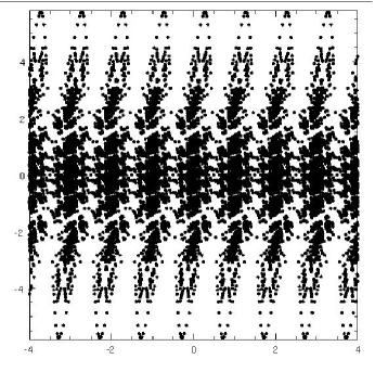
FIG. 3.: Each point corresponds to a periodic orbit. All fixed points up to order $n=5$ are shown. There are $19,624$ in all.

Numerically we count the number of boxes needed to cover the set as $\epsilon\rightarrow 0$. We measure the box-counting dimension as $2$, as predicted. To find the weighted dimensions we let $p_{i}$ equal the number of fixed points in a box and it is important to note that we count each time a given fixed point occurs, so short orbits are more heavily weighted. We find the information dimension is $D_{1}=1.4\pm 0.1$. The weight assigned to each box is sensitive to the number of windings around the space and therefore measures a different topological property than eqn. (17).

In the transition to quantum mechanics, remnants of chaos have been found in the form of smooth scars of enhanced amplitude along the classical periodic orbits [2]. We argue that the scars are the residue of the most frequently encountered orbits in the fractal set.

The semiclassical wave function can be constructed as a superposition of modes $\Psi(\vec{x})=\sum_{k}\hat{\phi}_{k}\psi_{k}(\vec{x})$ with $\psi_{k}$ eigenvectors of the Laplace-Beltrami operator, $\nabla^{2}\psi_{k}=-k^{2}\psi_{k}$. The intuition that the quantum system blurs any chaotic features derives from two important conjectures. The first conjecture asserts that the eigenvalues are given by random matrix theory for systems which are classically completely chaotic. As a consequence, the amplitudes $\hat{\phi}_{\vec{k}}$ are drawn from a Gaussian random ensemble with a flat spectrum and should be thoroughly mixed and featureless. The second conjecture, due to Berry [6], implies that the eigenmodes will be concentrated in the regions of phase space which are visited by the classical trajectories given an infinite time. A completely chaotic region of phase space is covered by mixing trajectories and at first glance Berry’s conjecture seems to imply a uniform distribution.

While these arguments for uniformity are convincing, one might wonder what happened to the structure of the periodic orbits. It is no surprise that the periodic orbits, which play such a prominent role in the classical dynamics, should also play a defining role in the quantum system. Periodic loops have in fact been the backbone of a quantization prescription in quantum chaos [4, 5]. Scars are the first evidence of quantum features related to these closed orbits. Heller discovered scars in the evolution of a wave-packet moving along a short orbit in a chaotic stadium [2]. He deduced that only certain eigenstates would contribute to the wave function as it traversed the orbit. Since the wave-packet was peaked about a single periodic orbit, the few contributing eigenstates must also show enhanced intensity along that orbit. The fewer the number of eigenstates which contribute to the wave-packet, the larger the intensity of the scar along that loop.

Rather than being inconsistent with Berry’s conjecture, the scar can be interpreted as a consequence of it. Scars occur in the regions of space where classical trajectories spend the most time. A typical trajectory will near a periodic orbit and then, due to the instability, will veer away onto a different periodic orbit. In this way, typical paths can be built from segments of periodic orbits. The most frequently visited periodic orbits tend to scar the most substantially. For a fully chaotic system, the fractal set of closed orbits will fill a volume in phase space. This would lead to some uniformity in the distribution of classical orbits and hence their quantum counterparts, as Berry suggested. However, not all closed orbits are created equal. Some may be visited by typical aperiodic trajectories more frequently than others.

The scarring phenomenon has been investigated primarily in terms of the dynamics of a wave-packet for test particle motion. Since the periodic orbits are unstable, a particle will depart from that trajectory by a factor of $\exp{(-\lambda t)}$ where $\lambda$ is the positive Lyapunov exponent. The frequency $\omega$ with which the wave-packet traces out the path must be sufficiently short, $\lambda/\omega\leq 1$, if the orbit is to be susceptible to scarring. For paths of length $\ell$, the frequency is $\omega=2\pi/\ell$. A hyperbolic surface is specified by $\lambda=1$ in curvature units and the scarring condition is simply $\ell\leq 2\pi$ [2, 8]. Only the shortest orbits scar. The short orbits are also the ones visited most frequently. The paths shown in fig. 1 are all of length $\ell\sim 3.06$ and are all potential avenues for scars.

On the compact octagon, the eigenmodes must obey precisely the same conditions as the periodic orbits: $\psi_{k}(\vec{x})=\psi_{k}(g_{j}\vec{x})$. The eigenmodes must be built out of primitives which correspond to the primitive periodic geodesics. For compact hyperbolic spaces, a relation between eigenmodes and closed loops is evident. Aurich and Steiner investigated scars in an asymmetric octagon in Refs [8]. They confirmed that the weighted spectral density of states shows bands related to the periodic recurrence of the wave packet along the orbit. The eigenstates under the bands had de Broglie wavelength, $\lambda_{B}\sim 2\pi/k$, a multiple of the length of the orbit, leading to the band quantization condition $k\sim{2\pi n\over\ell}$ for integer band quantum number $n$ [8]. The fewer the number of states contributing to a band, the more likely they were to show scars. Consistent with this observation, the authors found that very low energy eigenstates did scar short orbits. The low energy eigenstates had few orbits to choose from and therefore tended to show scars. (They found scars can appear as underdensities as well as overdensities [8].) For higher energy eigenstates however, they found that scars were absent. High-$k$ states have many orbits to choose from and so are less likely to scar along a given one. In fact, since $D_{q}=2$, we know that as $k\rightarrow\infty$, the area is covered by closed orbits. So, even if a given high-$k$ eigenstate aligns with some closed orbits, it will be entirely consistent with a random statistical distribution.

We should emphasize that a full description of the eigenmodes requires an infinite sum over orbits, or at least a very large and cautiously truncated sum. Still, we can guess the location of scars in physical space without this detailed description by exploiting the fractal connection. The scarred features can be described qualitatively for any classically chaotic system without having to quantize the system: simply isolate the most frequently visited orbits in the fractal set of periodic orbits. These will be the site for quantum scars. This offers a simple indicator of the quantum remnants of chaos.

A more strongly multifractal set would show more extreme scars than the weak scars on the octagon. But the compact space is interesting as a model of the universe and, like our universe, is suggestively marginal between homogeneity and inhomogeneity. If the octagon were a $2d$ universe, created in a Big Bang, then fluctuations in the geometry could be expanded in terms of the eigenmodes with amplitudes drawn from a random Gaussian ensemble with a flat spectrum. The superposition of fluctuations would show weak scars along short orbits from the low-$k$ modes but would appear increasingly random on smaller and smaller scales.

Since galaxies have their origin in quantum fluctuations, the distribution of large-scale structure would reflect the homogeneity on nearly all scales except the largest where the pattern of galaxies could carry memory of the quantum scars. On scales comparable to the area of the universe, the distribution of matter could appear filamentary and web-like.

Our own $3d$ universe does show vast voids and huge filaments in the distribution of large-scale structure. Galaxies would trace the scars and chart the shortest loops around a finite universe. If our universe is finite and negatively curved, the cobweb of luminous matter might be a residue of primordial quantum scars.

JDB and JL gratefully acknowledge PPARC support. We thank R. Aurich for useful comments.

REFERENCES

- [1] The entire volume Class. Quantum Grav. 15 9 (1998), Ed. G.D. Starkman.
- [2] E.J. Heller, Phys. Rev. Lett. 53 (1984) 1515.
- [3] N.L. Balazs and A. Voros, Phys. Rep. 143 (1986) 109.
- [4] M.C. Gutzwiller, J. Math. Phys., 12 (1971) 343.
- [5] M.V. Berry and M. Tabor, Proc. Roy. Soc. London, Ser. A 349 (1976) 101; J. Phys. A 10(1977) 371.
- [6] M.V. Berry, J. Phys. A 12 (1977) 2083; M.V. Berry in Chaotic Behavior of Deterministic Systems, eds. G. Iooss, R. Hellman, and R. Stora, Les Houches Proc. 36 (North-Holland, NY, 1981).
- [7] E. Ott, Chaos in dynamical systems, (CUP, Cambridge, 1993).
- [8] A. Aurich and F. Steiner, Physica D48 (1991) 445; Physica D64 (1993); 185. Chaos, Solitons & Fractals 5 (1995) 229.