Choptuik scaling in six dimensions

Abstract

We perform numerical simulations of the critical gravitational collapse of a spherically symmetric scalar field in 6 dimensions. The critical solution has discrete self-similarity. We find the critical exponent $\gamma$ and the self-similarity period $\Delta$.

I Introduction

Critical behavior in gravitational collapse, as first found by Choptuik[1], occurs at and near the threshold of black hole formation[2]. For a one-parameter family of initial data slightly above the threshold, the mass of the black hole, $M_{BH}$, scales like ${(p-p*)}^{\gamma}$. Here $p$ is the parameter, $p*$ is its critical value and $\gamma$ is a constant that depends on the type of matter, but not on the family of data. For initial data slightly below the threshold, the maximum curvature scales like ${(p*-p)}^{-2\gamma}$ where $\gamma$ is the same constant as in the black hole mass scaling law[3]. (The definition of the scaling exponent $\gamma$ must be slightly generalized in $n$ spacetime dimensions, where $M_{BH}$ has dimension $(\rm length)^{n-3}$; see section II.) The critical solution ($p=p*$) has either continuous self similarity or discrete self similarity, depending on the type of matter.

While critical gravitational collapse has been studied in many types of matter, the work has, in general, been done in 4 spacetime dimensions. (The exception is work on analogs of gravitational collapse in 3 spacetime dimensions[4]). One might therefore wonder whether critical behavior occurs in gravitational collapse in $n$ spacetime dimensions for $n>4$, and if so, how the properties of the critical behavior depend on $n$.

In this work, we perform numerical simulations of the collapse of a spherically symmetric scalar field in 6 spacetime dimensions. We find that the critical solution has discrete self-similarity. We find the scaling exponent $\gamma$ and the self-similarity period $\Delta$. Section 2 reviews the Schwarzschild solution in $n$ dimensions and shows how the definition of the $\gamma$ exponent should be generalized to the $n$-dimensional case. Section 3 gives the equations for the evolution of the scalar field and the metric in a form suitable for our numerical simulations. The numerical method is presented in section 4 and our results in section 5.

II Schwarzschild in $n$ dimensions

The Schwarzschild metric in $n$ spacetime dimensions is [5]

$$ds^{2}=-\bigl{(}1-\frac{16\pi}{(n-2)A_{n-2}}\frac{M}{r^{n-3}}\bigr{)}dt^{2}+\bigl{(}1-\frac{16\pi}{(n-2)A_{n-2}}\frac{M}{r^{n-3}}\bigr{)}^{-1}dr^{2}+r^{2}d\Omega^{2}_{n-2}$$ (1)

where $A_{n-2}=2\pi^{(n-1)/2}/\Gamma(\frac{n-1}{2})$ is the area of the unit $(n-2)$-sphere. The quantity $M$ in the metric (1) is the spacetime mass. M is normalized so that when (1) is the exterior metric of a nearly Newtonian static fluid ball, then $M$ is $\int{T_{00}dV}$. With this normalization, the force on a static unit-mass particle at distance $r$ approaches $\frac{8\pi(n-3)}{(n-2)A_{n-2}}M/r^{n-4}$ as $r\rightarrow\infty$.

It is important to note that $M$ has dimension $({\rm length})^{n-3}$. This implies the following scaling behaviors for critical phenomena in $n$ dimensions. If below threshold the maximum curvature [which has dimension $({\rm length})^{-2}$] scales like $(p*-p)^{-2\gamma}$, then above threshold $M_{BH}$ scales as $(p-p*)^{(n-3)\gamma}$.

III Evolution equations

Our matter model is the one used in reference[1]: a massless, minimally coupled, self gravitating scalar field $\phi$. The stress-energy of the field is

$${T_{ab}}={\nabla_{a}}\phi\,{\nabla_{b}}\phi\;-\;{1\over 2}\;{\nabla^{c}}\phi{\nabla_{c}}\phi\,{g_{ab}}$$ (2)

In $n$ spacetime dimensions, a spherically symmetric metric has the form

$$d{s^{2}}=-\;{e^{2\nu}}\,d{u^{2}}\;-\;2\,{e^{\nu+\lambda}}\,du\,dr\;+\;{r^{2}}d{\Sigma^{2}}$$ (3)

where $d{\Sigma^{2}}$ is the metric of the unit $(n-2)$-sphere and $\nu$ and $\lambda$ are functions of $u$ and $r$. The coordinate $r$ is a generalization of the usual area radius. The coordinate $u$ is constant on outgoing radial null geodesics. Here, we also require that on the world line of the central observer, $u$ is equal to the proper time of that observer. This gives rise to the condition $\nu=0$ at $r=0$. Define ${E_{ab}}\equiv{G_{ab}}\,-\,8\pi{T_{ab}}$ where $G_{ab}$ is the Einstein tensor, so the Einstein-scalar equations are just ${E_{ab}}=0$. Note that as a consequence of the Bianchi identities, $\phi$ must satisfy the wave equation.

In 4 spacetime dimensions, Christodoulou[8] showed how to write the spherically symmetric Einstein-scalar equations as an integro-differential equation for the scalar field. We now generalize the method of reference[8] to the $n$-dimensional case. Define the null vectors $l^{a}$ and $n^{a}$ by

$${l^{a}}={e^{-\lambda}}\;{{\left({\partial\over{\partial r}}\right)}^{a}}$$ (4)

$${n^{a}}={e^{-\nu}}\;{{\left({\partial\over{\partial u}}\right)}^{a}}\;-\;{1\over 2}\;{e^{-\lambda}}\;{{\left({\partial\over{\partial r}}\right)}^{a}}$$ (5)

Then some straightforward but tedious calculations give

$${G_{ab}}{l^{a}}{l^{b}}={{n-2}\over r}\;{e^{-2\lambda}}\;{\partial\over{\partial r}}\;(\lambda\,+\,\nu)\;\;\;,$$ (6)

$${G_{ab}}{l^{a}}{n^{b}}={{n-2}\over 2}\;\left[{{n-3}\over{r^{2}}}\;\left(1\,-\,{e^{-2\lambda}}\right)\;-\;{{e^{-2\lambda}}\over r}\;{\partial\over{\partial r}}\;(\nu\,-\,\lambda)\right]\;\;\;.$$ (7)

One can show that the equations

$${E_{ab}}{l^{a}}{l^{b}}=0\;\;\;\;,\;\;{E_{ab}}{l^{a}}{n^{b}}=0\;\;\;\;,\;\;\;{\nabla_{a}}{\nabla^{a}}\phi=0$$ (8)

plus the condition of regularity at the origin imply ${E_{ab}}=0$ everywhere. Thus we need to impose only those three equations.

Using equations (6,7) and (2), we find that the first two of equations (8) yield

$${{n-2}\over r}\;{\partial\over{\partial r}}\;(\lambda\,+\,\nu)\;-\;8\pi\;{{\left({{\partial\phi}\over{\partial r}}\right)}^{2}}=0\;\;\;.$$ (9)

$${{2-n}\over{2r}}\;\left[\;e^{-2\lambda}\;{\partial\over{\partial r}}\;(\nu\,-\,\lambda)-{{n-3}\over{r}}\;\left(1\,-\,{e^{-2\lambda}}\right)\;\right]=0\;\;\;.$$ (10)

Define $g\equiv{e^{\nu+\lambda}}$ and ${\bar{g}}\equiv{e^{\nu-\lambda}}$. Then the solution of equations (9) and (10) is

$$g=\exp\left[{{8\pi}\over{n-2}}\;{\int_{0}^{r}}\;{\hat{r}}\;{{\left({{\partial\phi}\over{\partial{\hat{r}}}}\right)}^{2}}\;d{\hat{r}}\right]\;\;\;.$$ (11)

$${\bar{g}}={{n-3}\over{r^{n-3}}}\;{\int_{0}^{r}}\;{{\hat{r}}^{n-4}}\;g(\hat{r})\;d\hat{r}\;\;\;.$$ (12)

The wave equation for $\phi$ in this metric is

$$2\;{{{\partial^{2}}\phi}\over{\partial u\partial r}}\;+\;{{n-2}\over r}\;{{\partial\phi}\over{\partial u}}\;-\;{r^{2-n}}\;{\partial\over{\partial r}}\;\left({r^{n-2}}\,{\bar{g}}\;{{\partial\phi}\over{\partial r}}\right)=0\;\;\;.$$ (13)

In principle, equations (11-13) could be used for a numerical treatment of the Einstein-scalar equations. Given $\phi$ on an initial light cone, equations (11) and (12) could be used to find the metric on that light cone. Equation (13) could then be used to evolve $\phi$ to a nearby light cone. However, in 4 spacetime dimensions, Christodoulou[8] finds that a change of variables gives rise to a nicer form of the wave equation. Define the operator $D$ by $D\equiv{e^{\nu}}{n^{a}}{\nabla_{a}}$. Then $D$ is a derivative along ingoing light rays and we have

$$D={\partial\over{\partial u}}\;-\;{1\over 2}\;{\bar{g}}\;{\partial\over{\partial r}}\;\;\;.$$ (14)

Now in 4 spacetime dimensions define $h\equiv({\partial/{\partial r}})(r\phi)$. Then the wave equation (13) becomes

$$D\,h={1\over{2r}}\;(g\,-\,{\bar{g}})\,(h\,-\,{\bar{h}})$$ (15)

where ${\bar{h}}\equiv{r^{-1}}{\int_{0}^{r}}h\,dr$. For the purposes of numerical simulations, the nice property of equation (15) is that it involves a derivative only in the direction of ingoing light rays. Another nice feature of equation (15) is that in the absence of gravity ($g={\bar{g}}=1$), the right hand side vanishes. This is related to the fact that in general, the right hand side vanishes like $r^{2}$ as $r\to 0$. (The metic is smooth, and therefore in a neighborhood of the origin it behaves like a flat metric to some order in $r$). This property is important for the following reason: spherically symmetric metrics have coordinate singularities at the origin. These coordinate singularities are reflected in the appearance of inverse powers of $r$ in equation (13), which can lead to instabilities or inaccuracies in a numerical simulation.

These considerations suggest that instead of a numerical simulation of equation (13) in $n$ dimensions, we should instead search for a new variable $h$ that satisfies $Dh=0$ in the absence of gravity. Note that a quantity that satisfies $Dh=0$ is constant along ingoing light rays and therefore satisfies Huygens’ principle. However, it is well known that solutions of the wave equation in flat spacetime satisfy Huygens’ principle only in even spacetime dimensions.[9] Therefore, we should only expect to find an appropriate new variable in even spacetime dimensions. Let $n$ be even and define $m\equiv(n-2)/2$. For any $\phi$ define

$$h\equiv{{(m-1)!}\over{(2m-1)!}}\;{r^{1-m}}\;{{\left({\partial\over{\partial r}}\right)}^{m}}\;\left({r^{2m-1}}\,\phi\right)\;\;\;.$$ (16)

(Here, the numerical factor is chosen for later convenience). If $\phi$ is a solution of the flat space wave equation (equation (13) with ${\bar{g}}=1$), then $h$ satisfies $Dh=0$. That is, in the absence of gravity, a solution of the wave equation $\phi$ gives rise to an $h$ that is constant along ingoing light rays. One can demonstrate this property of $h$ by using equation (13) (with ${\bar{g}}=1$) and mathematical induction on $m$.

The advantage of using $h$ as the basic variable is that it tends to make computer simulations more stable and accurate, especially near the origin. The disadvantages are (1) the method only works in even dimensions, (2) a seperate computer code must be written for each value of $n$ and (3) as $n$ gets larger, the equations become more complicated. We expect that some numerical technique can be used to evolve the Einstein-scalar equations in $n$ dimensions with a single code, with $n$ as a free parameter, stably and with enough accuracy to treat critical gravitational collapse. However, we have been unable to devise such a technique. Therefore, in this work we use $h$ as our basic variable. Due to the increase in complication with increasing $n$, we treat only the case of $6$ spacetime dimensions.

We now specialize to the case of 6 dimensions. The variable $h$ is given by

$$h\equiv{1\over{6r}}\;{{\partial^{2}}\over{\partial{r^{2}}}}\;\left({r^{3}}\,\phi\right)\;\;\;.$$ (17)

We must now use equation (11) to express $g$ in terms of $h$ and integrals involving $h$. Define the quantities $s$ and $\bar{s}$ by

$$s\equiv{2\over{r^{2}}}\;{\int_{0}^{r}}\;\hat{r}\;h(\hat{r})\;d\hat{r}\;\;\;,$$ (18)

$${\bar{s}}\equiv{3\over{r^{3}}}\;{\int_{0}^{r}}\;{\hat{r}^{2}}\;s(\hat{r})\;d\hat{r}\;\;\;.$$ (19)

Then, using equations (17-19) and (11) we find

$$g=\exp\left[18\,\pi\;{\int_{0}^{r}}\;{{d\hat{r}}\over{\hat{r}}}\;{{\left(s\,-\,{\bar{s}}\right)}^{2}}\right]\;\;\;.$$ (20)

Equation (12) specialized to 6 spacetime dimensions becomes

$${\bar{g}}={3\over{r^{3}}}\;{\int_{0}^{r}}\;{\hat{r}^{2}}\;g(\hat{r})\;d\hat{r}\;\;\;.$$ (21)

Using equations (17-21) in equation (13) we find that the wave equation for $\phi$ in 6 spacetime dimensions becomes

$$Dh={3\over r}\;(g\,-\,{\bar{g}})\,(h\,+\,{\bar{s}}\,-\,2s)\;+\;{{27\pi}\over 2}\;{g\over r}\;{{(s\,-\,{\bar{s}})}^{3}}\;\;\;.$$ (22)

Equations (17-22) are the full set of equations that are evolved in 6 spacetime dimensions.

IV Numerical method

The numerical method used is that of Garfinkle[6]. This method is based on numerical work of Goldwirth and Piran[7], which is in turn based on the analytical work of Christodoulou[8]. The spatial grid is a set of points on an outgoing null cone, and each spatial grid point is evolved along an ingoing light ray. Given $h$ on a light cone, the code performs several integrals in turn: equations (18-21). Near the origin, these integrals are approximated by a Taylor series and evaluated using the slope of $h$ at $r=0$. At all other points, the integrals are evaluated using Simpson’s rule.

For each time step the quantity $h$ is evolved using equation (22) and the quantity $r$ is evolved using

$$Dr=-\;{{\bar{g}}\over 2}\;\;\;.$$ (23)

These are essentially a set of uncoupled ODEs, one for each grid point. In the scheme of[6] as the evolution procedes grid points that pass through $r=0$ are lost. When half of the grid points are lost, they are put back, interpolated between the remaining grid points. The critical solution is found by a search of a $1$-parameter space of evolved data to find the boundary between those data that form black holes and those that do not. The outermost gridpoint is chosen to be the light ray that hits the singularity of the critical solution. This choice maintains resolution throughout the evolution.

V Results

All runs were done with 300 spatial grid points. The code was run in quadruple precision on Dec alpha workstations and in double precision on a Cray YMP8. The initial data for the scalar field was chosen to be of the form

$$\phi(0,r)=p\;{r^{2}}\;\exp\left[-\;{{(r-{r_{0}})}^{2}}/{\sigma^{2}}\right]\;\;\;.$$ (24)

Here, $p$ is our parameter, and $r_{0}$ and $\sigma$ are constants. The critical solution was found to have discrete self-similarity. Let $u*$ be the value of $u$ at the origin at the singularity of the critical solution. Define the coordinates $T\equiv-\ln(u*-u)$ and $R\equiv r{e^{T}}$. Then discrete self similarity means that $h$, considered as a function of $T$ and $R$, is periodic in $T$. Figure 1 shows $h$ plotted as a function of $T$ and $R$. Note that after some initial transient behavior, $h$ becomes periodic. To examine the periodicity more closely, in Figure 2 we plot $h$ vs $R$ at two different times where the minimum of $h$ occurs at $r=0$. Note that the curves agree, demonstrating periodicity of $h$. The period of $h$ is $\Delta=3.03$. Thus, in each period a typical length of the system shrinks by a factor of ${e^{\Delta}}\approx 21$. For comparison, recall that for $n=4$, $\Delta=3.445$.

To compute the scaling exponent $\gamma$ we use the method of reference[3]. We evolve data for a range of parameters below the threshold of black hole formation. For each evolution we find the maximum of the absolute value of the scalar curvature on the world line of the central observer $R_{\rm max}$. Plotting $\ln{R_{\rm max}}$ vs $\ln(p*-p)$ the result is a straight line with a periodic wiggle, where the slope of the line is $-\,2\gamma$. We use 50 values of $p$ equally spaced in $\ln(p*-p)$. Figure 3 is a plot of $\ln{R_{\rm max}}$ vs $\ln(p*-p)$ along with the best straight line fit to the points. The slope allows us to find $\gamma$. The result is $\gamma=0.424$, so $M_{BH}\propto(p-p*)^{1.27}$. Recall that for $n=4$, $\gamma=0.374$. Note that $\gamma$ can also be found by evolving data above the threshold of black hole formation and plotting $\ln{M_{BH}}$ vs $\ln(p-p*)$. We have done this and the result is a straight line with a periodic wiggle where the slope of the line is $\approx 1.27$. However, our method gives a more accurate treatment of subcritical collapse than of supercritical collapse. For that reason, we have used subcritical collapse to calculate $\gamma$.

Comparison of our results for 6 dimensions with Choptuik’s results for 4 dimensions[1] seems to indicate that $\Delta$ is a decreasing function of the dimensionality $n$ of spacetime. The quantity $\gamma$ seems to be an increasing function of $n$. It would be interesting to obtain more information about these functions by studying critical collapse for other values of $n$.

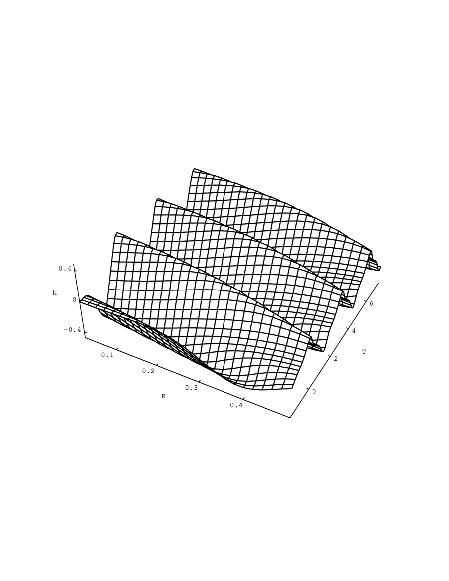
FIG. 1.: $h$ plotted vs. the rescaled coordinates $R$ and $T$.

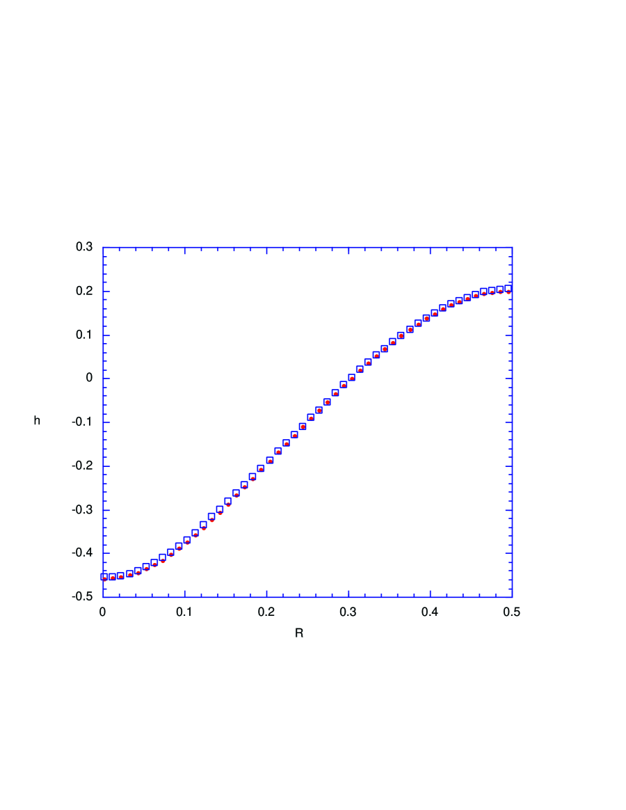
FIG. 2.: $h$ plotted vs. $R$ at two times when the minimum of $h$ is at $r=0$. Note that the two curves agree.

FIG. 3.: $\ln{R_{\rm max}}$ plotted vs. $\ln(p*-p)$ along with the best straight line fit. The curve is a straight line with a periodic wiggle and the slope of the line is $-2\gamma$.

- [1] M. Choptuik, Phys. Rev. Lett. 70, 9 (1993)
- [2] For a review see C. Gundlach, Adv. Theor. Math. Phys. 2, 1 (1998) and references therein
- [3] D. Garfinkle and G.C. Duncan, Phys. Rev. D 58, 064024 (1998)
- [4] Y. Peleg and A. Steif, Phys. Rev. D51, 3992 (1995)
- [5] R. Myers and M. Perry, Ann. Phys. 172, 304 (1986)
- [6] D. Garfinkle, Phys. Rev. D51, 5558 (1995)
- [7] D.S. Goldwirth and T. Piran, Phys. Rev. D36, 3575 (1987)
- [8] D. Christodoulou, Commun. Math. Phys. 105, 337 (1986)
- [9] Y. Choquet-Bruhat, C. De Witt-Morette and M. Dillard-Bleick, Analysis, Manifolds and Physics, page 432 (North Holland, Amsterdam, 1977)