Detection of Gravitational Waves from Eccentric Compact Binaries

Abstract

Coalescing compact binaries have been pointed out as the most promising source of gravitational waves for kilometer-size interferometers such as LIGO. Gravitational wave signals are extracted from the noise in the detectors by matched filtering. This technique performs really well if an a priori theoretical knowledge of the signal is available. The information known about the possible sources is used to construct a model of the expected waveforms (templates). A common assumption made when constructing templates for coalescing compact binaries is that the companions move in a quasi-circular orbit. Some scenarios, however, predict the existence of eccentric binaries. We investigate the loss in signal-to-noise ratio induced by non-optimal filtering of eccentric signals.

1 Introduction

Coalescing compact binaries have been pointed out as the most promising source of gravitational waves for the LIGO/VIRGO/TAMA/GEO interferometers[1, 2]. These binaries typically have formed a long time ago, giving them time to radiate most of their eccentricity away. The templates (model of the radiation) needed for matched filtering are thus constructed according to this assumption. Gravitational waves emitted by a circular binary will be explicitly searched for in the output of the detectors, but not gravitational waves emitted by eccentric binaries. The scenario we have in mind allows for the formation of young eccentric binary systems, young enough that they did not have had time to be fully circularized by the radiation reaction. For example, the collapse of a dense Newtonian globular cluster can lead to the formation of a copious number of eccentric binaries via two- and three- body encounters[3, 4].

These eccentric binaries will emit strongly in the frequency band of the LIGO interferometers. It may seem that these eccentric binaries can be dealt with by incorporating adequate templates in the bank of templates already available, but this may prove to be inefficient. The addition of new templates has two undesirable effects: It adds to the already heavy computational burden associated with data processing and it increases the probability of false detection (mistaking the noise in the detector for a signal). A better solution might be to search for these eccentric signals with the circular templates, and once a signal is concluded to be present, to extract the information using eccentric templates.

For this to be possible, the circular templates have to follow the phase of the eccentric signals very well. To assess the quality of the circular templates at modeling eccentric signals, special detection tools are needed.

2 Matched filtering as a detection method

Gravitational wave signals are very weak and at best they will be of the same order of magnitude as the noise in the detectors. This motivates the general belief that matched filtering will be needed to extract the signals from the noisy output of the detectors [1]. When the signals are of known shape, this technique produces the highest signal-to-noise ratio[5]. Suppose a gravitational wave $h(t)$ reaches the detector. The output of the detector $o(t)$ is then a superposition of the useful signal $h(t)$ and the noise $n(t)$. In matched filtering, the signal is extracted by using a theoretical template (theoretical model) that mimics the signal as well as possible; we call this template $m(t,\mbox{\boldmath$\Omega$\unboldmath})$. The vector $\Omega$ denotes the parameters that characterize the template. If the template were a perfect copy of the signal, the parameters would represent the real parameters of the source, such as its mass and distance from earth. If the templates are not a perfect approximation to the real signal, the parameters $\Omega$ represent phenomenological parameters.

If instead of working in the time domain we work in frequency space, we can introduce the natural inner product of matched filtering. For two functions $a(t)$ and $b(t)$ with Fourier transforms $\tilde{a}(f)$ and $\tilde{b}(f)$, the inner product is defined as[6]

$$(a|b) = 2\int_{0}^{\infty}{\mathrm{d}}f\frac{\tilde{a}^{*}(f)\tilde{b}(f)+\tilde{a}(f)\tilde{b}^{*}(f)}{S_{n}(f)}\,,$$ (1)

where a “  *  ” denotes complex conjugation and $S_{n}(f)$ is the one-sided spectral density of the detector’s noise. In terms of this inner product, the average signal to noise ratio is[7]

$$\left<\rho\right> = \frac{(m(\mbox{\boldmath$\Omega$\unboldmath})|h)}{\sqrt{(m(\mbox{\boldmath$\Omega$\unboldmath})|m(\mbox{\boldmath$\Omega$\unboldmath}))}}\,.$$ (2)

In practice, the set of parameters $\Omega$ is varied until a maximum of the signal-to-noise ratio is found. This maximum is the signal-to-noise ratio achievable by using $\tilde{m}(f,\mbox{\boldmath$\Omega$\unboldmath})$ as a template. The signal-to-noise ratio of equation (2) does not give any information about the quality of the templates or, equivalently, how well the template models the signal. The Schwartz inequality provides an answer to this question[7]. The absolute maximum the signal-to noise ratio can take is achieved when the template is a perfect match of the signal, and the parameters $\Omega$ correspond to the parameters of the source ($\tilde{m}(t,\mbox{\boldmath$\Omega$\unboldmath})\equiv\tilde{h}(f)$). The optimal SNR is[7]

$$\left<\rho\right>_{max} = \sqrt{(h|h)}\,.$$ (3)

By dividing the signal-to-noise ratio (equation (2)) with the value achieved by optimal filtering (equation (3)), we construct the ambiguity function ${\mathcal{A}}(\mbox{\boldmath$\Omega$\unboldmath})$:

$${\mathcal{A}}(\mbox{\boldmath$\Omega$\unboldmath}) = \frac{(m(\mbox{\boldmath$\Omega$\unboldmath})|h)}{\sqrt{(m(\mbox{\boldmath$\Omega$\unboldmath})|m(\mbox{\boldmath$\Omega$\unboldmath}))(h|h)}}\,.$$ (4)

This function takes values between 0 and 1. It is equal to 1 when the optimal template is used.

The value of the parameters $\Omega$ can be varied until ${\mathcal{A}}(\mbox{\boldmath$\Omega$\unboldmath})$ is maximized. The maximum value of the ambiguity function is the fitting factor:

$$FF=\max_{\mbox{\boldmath$\Omega$\unboldmath}}{\mathcal{A}}(\mbox{\boldmath$\Omega$\unboldmath})\,.$$ (5)

The fitting factor is a direct measure of the template’s quality since it can be related to the loss of event rate, i.e. the number of events missed by using an inappropriate set of templates. This loss is calculated according to $1-FF^{3}$[6]. For example, if the fitting factor is 0.8, then $48.8\%$ of the events would be mistaken for noise. We adopt a threshold of $FF=0.9$ for the present work. This corresponds to a loss in event rate of $27\%$.

3 The gravitational waveforms

We calculate the waveforms for both circular and eccentric binaries in the quadrupole approximation. In this approximation the waveforms are given by[8]

$$h^{TT}_{ij}=\frac{2}{R}\frac{{\mathrm{d}}^{2}}{{\mathrm{d}}t^{2}}\left(I_{ij}-\frac{1}{3}\delta_{ij}I^{k}\,_{k}\right)^{TT}\,,$$ (6)

where $R$ is the distance between the source and the observer, $I_{ij}$ is the source’s quadrupole moment and the superscript $TT$ reminds us that gravitational waves are traceless and live in the plane transverse to the direction of propagation.

For eccentric binary systems, the waveforms are[9]

$$\mathrm{h_{+}} = h_{xx}=-h_{yy}=\frac{1}{R}\frac{\mu}{p}\Bigg{\{}2(1+\cos^{2}\theta_{o})\cos 2(\varphi-\varphi_{o})$$ (7)

$$+ e\left[(1+\cos^{2}\theta_{o})\left(\frac{5}{2}\cos(\varphi-2\varphi_{o})+\frac{1}{2}\cos(3\varphi-2\varphi_{o})\right)+\sin^{2}\theta_{o}\cos\varphi\right]$$

$$+ e^{2}{(1+\cos^{2}\theta_{o})\cos 2\varphi_{o}+\sin^{2}\theta_{o}}\Bigg{\}}\,,$$

$$\mathrm{h_{\times}} = h_{xy}=h_{yx}=-\frac{1}{R}\frac{\mu}{p}\cos\theta_{o}\Bigg{\{}4\sin 2(\varphi-2\varphi_{o})$$ (8)

$$+ e\left[5\sin(\varphi-2\varphi_{o})+\sin(3\varphi-2\varphi_{o})\right\}-2e^{2}\sin 2\varphi_{o}\Bigg{\}}\,,$$

where $\theta_{o}$ and $\varphi_{o}$ are the two angles defining the location of the observer with respect to the orbital plane, $\mu$ is the reduced mass, and $p$ and $e$ are defined in terms of the turning points $(r_{\pm})$ of the Newtonian orbit as

$$r_{\pm} = \frac{Mp}{1\pm e}\,.$$

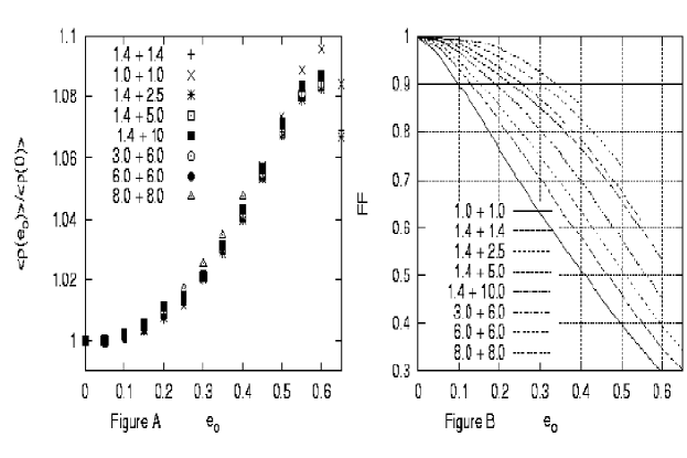
Figure 1: Figure A: The ratio of the optimal signal-to-noise ratio $\left<\rho(e_{o})\right>$ to the signal-to-noise ratio ($\left<\rho(0)\right>$). The figure shows that eccentric binary systems will be easier to detect if they are explicitly searched for at the output of the interferometers.
Figure B: The fitting factor as a function of $e_{o}$ for various binary systems. Two trends are apparent. The first one is the net decrease in the fitting factor as $e_{o}$ increases, while the total mass of the binary is held fixed. The second one is the increase in the detection probability when the total mass of the binary increases. The various binaries studied are labeled by the two masses of the companions; they are given in units of the solar mass.

The eccentric waveforms oscillate at once, twice and thrice the orbital frequency, whereas the circular waveforms oscillate only at twice the orbital frequency. We parameterize our binaries by specifying the two masses, and the eccentricity $e_{o}$ they have when they first enter the LIGO frequency band (at 40 Hz).

The Fourier transform of the waveforms is calculated numerically for the eccentric signal, and obtained through the stationary phase approximation for the circular templates[10]. Once these Fourier transforms are known, it is straightforward to calculate the optimal SNR (equation (3)), build the ambiguity function (equation (4)), and maximize it over the different parameters of the templates to get the fitting factor (equation (5)).

The results for the signal-to noise ratio and the fitting factor are displayed in figure (1). The signal-to-noise ratio for an eccentric signal is higher than the ratio obtained for an equivalent circular binary. This means that if both binaries are located at the same distance $R$, the eccentric binary will emit stronger radiation and will be easier to detect if optimal filters are used. On the other hand, the fitting factor decreases as the initial eccentricity is increased. The circular templates fail to model the eccentric signal properly. The good news is that circular templates are still accurate enough to detect some eccentric signals. For example, a neutron star binary system will be detected as long as its initial eccentricity does not exceed 0.13. If the total mass of the system is increased, the detection probability increases as well. For example, for a system of two 8.0 $M_{\odot}$ black holes, the initial eccentricity can be as high as 0.33. This trend is explained in the following way. As the total mass of the system increases, the radiation it emits is stronger and the system coalesces in a shorter time. The shorter the signal, the less opportunity the circular templates have to go out of phase with it. This is a good news, because the higher the mass is, the easier it is to detect the signal because it is stronger. Thus, the LIGO interferometers should be able to detect radiation from some eccentric binaries, those with large masses and relatively low eccentricities[11].

Acknowledgments: This work was carried out with É. Poisson. It was supported by NSERC.

References

- [1] K.S. Thorne. Three Hundred Years of Gravitation, pages 330–458. Cambridge University Press, New York(1987).
- [2] B.F. Schutz. Gravitational waves. Nuclear Physics B35(Proc. Suppl.), 44(1994).
- [3] S.L. Shapiro and S.A. Teukolsky. The collapse of dense star clusters to supermassive black holes: The origin of quasars and AGN’s. Astrophys. J. 292, L41(1985).
- [4] S.L. Shapiro and G.D. Quinlan. The collapse of dense star clusters to supermassive black holes: Binaries and gravitational radiation. Astrophys. J. 321, 199(1987).
- [5] . . Flanagan and S. A. Hughes. Measuring gravitational waves from binary black hole coalescences: I. signal to noise for inspiral, merger, ringdown. Phys.Rev. D57, 4535(1998).
- [6] T.A. Apostolatos. Construction of a template family for the detection of gravitational waves from coalescing binaries. Phys.Rev.D54, 2421(1996).
- [7] L.A. Wainstein and V.D. Zubakov. Extraction of Signals from Noise. Prentice-Hall, Englewood Cliffs (1962).
- [8] C.W. Misner, K.S. Thorne, and J.A. Wheeler. Gravitation. Freemann, San Francisco(1973).
- [9] H. Wahlquist. The doppler response to gravitational waves from a binary star source. General Relativity and Gravitation, vol.19, no 11, 1101(1987).
- [10] L.S. Finn and D.F. Chernoff. Observing binary inspiral in gravitational radiation: One interferometer. Phys. Rev. D47, 2198(1993).
- [11] K. Martel and . Poisson. http://xxx.lanl.gov/archive/gr-qc, 9907006.