Self-similar cosmological solutions with a non-minimally coupled scalar field

Abstract

We present self-similar cosmological solutions for a barotropic fluid plus scalar field with Brans-Dicke-type coupling to the spacetime curvature and an arbitrary power-law potential energy. We identify all the fixed points in the autonomous phase-plane, including a scaling solution where the fluid density scales with the scalar field’s kinetic and potential energy. This is related by a conformal transformation to a scaling solution for a scalar field with exponential potential minimally coupled to the spacetime curvature, but non-minimally coupled to the barotropic fluid. Radiation is automatically decoupled from the scalar field, but energy transfer between the field and non-relativistic dark matter can lead to a change to an accelerated expansion at late times in the Einstein frame. The scalar field density can mimic a cosmological constant even for steep potentials in the strong coupling limit.

]

I Introduction

Scalar fields have come to play a dominant role in recent years in theoretical models of the universe. This has usually been in the context of inflationary models of the very early universe where the self interaction potential energy density $V(\phi)$ remains undiluted by the cosmological expansion. If the potential is sufficiently flat this can lead to an effective cosmological constant which can drive an accelerated expansion. The detailed nature of the evolution is driven by the specific form of the scalar field’s potential energy.

More recently observational evidence has been growing that the energy density of the universe today may be dominated by a homogeneous (smooth) component with negative pressure - christened “quintessence” [1]. A suitably small cosmological constant $\Lambda$ provides a good fit to the observational data [2, 3], but the required low energy scale, $\Lambda\sim(10^{-3}{\rm eV})^{4}$, seems unnatural in any supergravity model. This has lead to an explosion of interest in the late-time evolution of self-interacting scalar fields, where radiation and matter contribute the dominant energy density at earlier times, but slowly rolling scalar fields may provide a dynamical mechanism to achieve a small effective cosmological constant today by mimicking a decaying effective-$\Lambda$. The late time evolution of sufficiently steep potentials has been shown to be largely insensitive to initial conditions [4] (though it should be remembered that it the case of a true cosmological constant there is also no dependence upon initial conditions!). This steep potential must become flat by the present in order to act as an effective cosmological constant today and there remains the “fine-tuning” problem of why the scalar field density comes to dominate at just the present epoch.

Scalar fields with exponential potentials provide a strikingly simple model in which the energy density of the scalar field decreases at exactly the same rate as a barotropic fluid. Wetterich [5] was the first to point out that the energy density of a scalar field with an exponential potential does not simply die away if the potential is too steep to drive inflation, but rather approaches an attractor solution [6] where it mimics the equation of state of a barotropic fluid (radiation or dust) and remains a fixed fraction of the total energy density. We will refer to these solutions as self-similar or scaling cosmological models where the dimensionless density parameter for each component, $\Omega_{i}\equiv\rho_{i}/\rho_{\rm crit}$, is a constant.

Self-similar homogeneous cosmological solutions are invariant under a global conformal rescaling of the metric. Such models may be expanding, but the physical state at different times differ only by a change in the overall length scale [8]. In a Friedmann-Robertson-Walker (FRW) cosmological model this is equivalent to a rescaling of the cosmic time,

$$t\to\Gamma t\ ,$$ (1)

where $\Gamma$ is a constant. Self-similarity requires that the evolution of the scale factor $a(t)$ is a power-law, and the Hubble constant $H\equiv\dot{a}/a\propto 1/t$.

We will consider the evolution of spatially flat FRW cosmologies containing a fluid, with density $\rho$, and pressure $P$, and a scalar field $\phi$ with self-interaction potential $V(\phi)$. In general relativity, the Friedmann constraint equation requires

$$H^{2}={8\pi G_{N}\over 3}\left(\rho+{1\over 2}\dot{\phi}^{2}+V(\phi)\right)\ ,$$ (2)

where $G_{N}$ is Newton’s constant. Equation (1) then requires that the matter content is invariant under a rescaling $\rho\to\Gamma^{-2}\rho$. Requiring $P\to\Gamma^{-2}P$ for all $\Gamma$ then leads to a barotropic equation of state $P=(\gamma-1)\rho$ where $\gamma$ is a constant. Thus the familiar radiation ($\gamma=4/3$) or pressureless matter ($\gamma=1$) dominated FRW models can be described as self-similar solutions with

$$a\propto t^{2/(3\gamma)}\ .$$ (3)

A scalar field has kinetic energy $\dot{\phi}^{2}/2$ which only allows a constant shift of the scalar field, $\phi\to\phi+\phi_{\Gamma}$, if we are to require $\dot{\phi}^{2}\to\Gamma^{-2}\dot{\phi}^{2}$. In order to obtain a self-similar solution we require in addition

$$V(\phi)\to V(\phi+\phi_{\Gamma})=\Gamma^{-2}V(\phi)\ .$$ (4)

which is only compatible with a non-interacting field, $V(\phi)=0$, or an exponential potential

$$V(\phi)=V_{0}\exp\left(-\lambda\kappa\phi\right)\ ,$$ (5)

where $\kappa^{2}=8\pi G_{N}$, $\lambda$ is a dimensionless constant and we have $\kappa\phi_{\Gamma}=(2/\lambda)\ln\Gamma$.

FRW solutions for scalar fields with exponential potentials where the kinetic energy and potential energy of the field remain proportional were proposed as a model for power-law inflation in the early universe by Luchinn and Matarrese [9], and are the late-time attractor solutions (in the absence of other matter) for $\lambda^{2}<6$ [10, 11]. More recently attention has focused on the possible late-time evolution of scalar fields in FRW cosmologies containing matter. Self-similar solutions are known for scalar fields with exponential potentials whose energy density scales with that of a barotropic fluid yielding the same time dependence given in Eq. (3) for a barotropic fluid dominated solution [5]. These scaling solutions are the unique late-time attractors for sufficiently steep potentials ($\lambda^{2}>3\gamma$) [6]. Such a scalar field is so successful at scaling with the barotropic matter that the scalar field never comes to dominate the cosmological dynamics. A minimally coupled field can only mimic a cosmological constant at late times if the scale invariance of the scalar field is broken, leading to the deviation from the pure scaling solution which must be fine-tuned to occur at just the present epoch.

In this paper we will consider the effect of non-minimal coupling of the scalar field to the spacetime curvature. In the next section we show that self-similar cosmological solutions are possible for scalar fields with simple power-law potentials if the scalar field has a Brans-Dicke-type coupling to the spacetime curvature. The equations of motion reduce to an autonomous phase-plane whose fixed points correspond to self-similar solutions. We show that this system is conformally related to a scalar field with exponential potential and minimally coupled to the spacetime curvature, but with an explicit coupling to matter, studied in Refs. [12, 13, 14, 15, 16]. This coupling is sensitive to the fluid equation of state and can produce a natural change in the nature of the solution after matter-radiation equality. In contrast with the case of a minimally coupled scalar field there is the possibility of recovering an effective late time cosmological constant even if the potential remains steep [17], depending on the value of the dimensionless non–minimal coupling constant and we investigate this possibility in section III.

II Brans–Dicke–type cosmology with power–law potential

It is possible to obtain self-similar solutions for scalar fields with arbitrary power-law potentials , $V(\phi)=V_{0}(\kappa\phi)^{2n}$, if we go beyond Einstein’s theory of general relativity and allow the field to be non-minimally coupled to the spacetime curvature. In Brans-Dicke gravity [18] with dimensionless parameter $\omega$, Newton’s constant is replaced by a dynamical field $G=\omega/(2\pi\phi^{2})$ and the generalised Friedmann equation requires

$$H^{2}={8\pi\over 3}{\omega\over 2\pi\phi^{2}}\left(\rho+{1\over 2}\dot{\phi}^{2}+V(\phi)-{3\over 2\omega}H\phi\dot{\phi}\right)\ .$$ (6)

In the original Brans-Dicke theory where $V(\phi)=0$, Eq. (1) is compatible with a global re-scaling of the barotropic fluid density $\rho\to\Gamma_{\rho}\rho$ and $\phi\to\Gamma_{\phi}\phi$ for all $\Gamma_{\rho}/\Gamma_{\phi}^{2}=\Gamma^{-2}$. The self-similar solution for a barotropic fluid in Brans-Dicke gravity was given by Nariai [20, 21]. In the presence of a power-law potential, $V(\phi)=V_{0}(\kappa\phi)^{2n}$, (absent in the pure Brans-Dicke theory [18]) we require in addition that $V(\phi)/\phi^{2}\to\Gamma^{-2}[V(\phi)/\phi^{2}]$ which specifies $\phi\to\Gamma^{-1/(n-1)}\phi$ and $\rho\to\Gamma^{-2n/(n-1)}\rho$. Thus self-similar solutions can exist for “quintessence”-type power-law scalar field potentials [22, 23], so long as this scalar field has Brans-Dicke type coupling to the spacetime curvature.

Motivated by the preceding qualitative discussion of self-similar solutions we examine the cosmological evolution of one of the simplest forms of non–minimal coupling proposed by Brans and Dicke [18] which is described by a single dimensionless parameter $\omega$. In addition to the original Brans–Dicke Lagrangian [18], we introduce a self interaction potential $V(\phi)$ [24, 25, 26, 27]. The action is

$$S = \int\sqrt{-g}d^{4}x[\pm{1\over 8\omega}\phi^{2}R\mp\frac{1}{2}g^{\mu\nu}\phi_{,\mu}\phi_{,\nu}-V(\phi)]\,$$ (7)

$$+ \int\sqrt{-g}d^{4}x{\cal L}_{matter}\,$$ (8)

where upper/lower signs should be chosen to ensure $\pm\omega>0$ and hence a positive gravitational coupling. The self-interaction potential is taken to be a power-law,

$$V(\phi)=V_{0}(\kappa\phi)^{2n}\ .$$ (9)

This action can be re-expressed as a theory of interacting matter fields in general relativity with fixed Newton’s constant $G_{N}$ [28] if we define quantities in the conformally related Einstein frame with respect to the rescaled metric

$$\tilde{g}_{\mu\nu}=\left|{\kappa^{2}\phi^{2}\over 4\omega}\right|g_{\mu\nu}\ .$$ (10)

The scalar field is now minimally coupled to metric $\tilde{g}_{\mu\nu}$, but non-minimally coupled to the other matter fields. We will re-express the scalar field $\phi$ in terms of a field $\psi$ which has a canonical kinetic term in the Einstein frame, which requires that

$$\kappa\phi=\exp\left({\kappa\psi\over\sqrt{2(3+2\omega)}}\right)\ .$$ (11)

The scalar field will have a non-negative energy density in the Einstein frame so long as $\omega>-3/2$. Thus we consider $\omega$ with any value $>-3/2$, which includes, for example, the coupling of the string-theory dilaton where $\omega=-1$ [29].

The effective self-interaction potential for canonical field $\psi$ in the Einstein frame is of exponential form and given by (see, e.g., Refs. [27, 30])

$$\tilde{V}(\psi)=\left(\frac{4\omega}{\kappa^{2}\phi^{2}}\right)^{2}V(\phi)=\tilde{V}_{0}\exp(-\lambda\kappa\psi)\ ,$$ (12)

where $\tilde{V}_{0}\equiv(4\omega)^{2}V_{0}$ and

$$\lambda\equiv\sqrt{{2\over 3+2\omega}}(2-n)\ .$$ (13)

A Autonomous Phase–Plane

Using the Hubble rate, $\tilde{H}$, fluid density, $\tilde{\rho}$, and scalar field density, $\tilde{\rho}_{\psi}=(1/2)(d\psi/d\tilde{t})^{2}+\tilde{V}(\psi)$, defined in the Einstein frame, the evolution equations are

$$\frac{d\tilde{H}}{d\tilde{t}}=-\frac{\kappa^{2}}{2}\left(\tilde{\rho}+\tilde{P}+\left(\frac{d\psi}{d\tilde{t}}\right)^{2}\right)\,,$$ (14)

$$\frac{d\tilde{\rho}}{d\tilde{t}}+3\tilde{H}(\tilde{\rho}+\tilde{P})=-\frac{dQ}{d\tilde{t}}\,,$$ (15)

$$\frac{d\psi}{d\tilde{t}}\left(\frac{d^{2}\psi}{d\tilde{t}^{2}}+\frac{d\tilde{V}}{d\psi}+3\tilde{H}\frac{d\psi}{d\tilde{t}}\right)=\frac{dQ}{d\tilde{t}}\,,$$ (16)

subject to the Friedmann constraint,

$$\tilde{H}^{2}=\frac{\kappa^{2}}{3}\left(\tilde{\rho}+\frac{1}{2}\left(\frac{d\psi}{d\tilde{t}}\right)^{2}+\tilde{V}(\psi)\right).$$ (17)

The non-minimal coupling of the scalar field in the Brans-Dicke frame leads to an explicit energy transfer in the Einstein frame, between the scalar field and the fluid,

$$\frac{dQ}{d\tilde{t}}\equiv\kappa\frac{d\psi}{d\tilde{t}}\frac{\tilde{\rho}-3\tilde{P}}{\sqrt{2(3+2\omega)}}\,.$$ (18)

The same system of equations was considered, starting from a different motivation, by Wetterich [13], and more recently by Amendola [14]. In the case $dQ/d\tilde{t}=0$, these equations reduce to previous studies of minimally coupled scalar fields with exponential potentials [5, 6].

Following Ref. [6], we define,

$$x\equiv\frac{\kappa}{\sqrt{6}\tilde{H}}\left(\frac{d\psi}{d\tilde{t}}\right)\qquad,\qquad y\equiv\frac{\kappa\sqrt{\tilde{V}}}{\sqrt{3}\tilde{H}}\,.$$ (19)

The evolution equations for a barotropic fluid where $\tilde{P}=(\gamma-1)\tilde{\rho}$ can then be written as [6, 14]

$$x^{\prime} = -3x+\lambda\sqrt{\frac{3}{2}}y^{2}+\frac{3}{2}x[2x^{2}+\gamma(1-x^{2}-y^{2})]\,$$ (20)

$$+ W(1-x^{2}-y^{2}),$$ (21)

$$y^{\prime} = -\lambda\sqrt{\frac{3}{2}}xy+\frac{3}{2}y[2x^{2}+\gamma(1-x^{2}-y^{2})],$$ (22)

where a prime denotes the derivative with respect to $N\equiv\int\tilde{H}d\tilde{t}$, the logarithm of the scale factor in the Einstein frame, and we have used the constraint equation,

$$\frac{\kappa^{2}\tilde{\rho}}{3\tilde{H}^{2}}+x^{2}+y^{2}=1$$ (23)

We parameterise the energy transfer in terms of the dimensionless quantity $W$, where

$$W\equiv\sqrt{\frac{3}{3+2\omega}}\left(\frac{4-3\gamma}{2}\right)\ ,$$ (24)

Equations (20) and (22) define an two-dimensional autonomous phase-plane whenever $W$ can be written as function of $x$ and $y$. The Brans-Dicke-type theory defined in Eq. (7) naturally leads to an interaction with constant $W$, although the analysis could be extended to more general $W(x,y)$ [15, 16].

The constraint Eq. (23) restricts physical solutions with non–negative fluid density to $0\leq x^{2}+y^{2}\leq 1$ and so the evolution is completely described by trajectories within the unit disc. In the following discussion we will only consider expanding cosmologies corresponding to the upper-half disc, $y\geq 0$.

B Self-similar solutions

Fixed points of the system, ($x_{i}$,$y_{i}$) where $x^{\prime}=0$ and $y^{\prime}=0$, correspond to power-law solutions for the scale factor and logarithmic evolution of the scalar field with respect to the cosmic time in the Einstein frame:

$$\tilde{a}\propto\tilde{t}^{\tilde{p}}\quad,\quad\kappa\psi\propto\tilde{q}\ln\tilde{t}\,,$$ (25)

where the constants $\tilde{p}$ and $\tilde{q}$ are given by,

$$\tilde{p} = \frac{2}{3\gamma(1-x_{i}^{2}-y_{i}^{2})+6x_{i}^{2}}\,,$$ (26)

$$\tilde{q} = \frac{2\sqrt{6}x_{i}}{3\gamma(1-x_{i}^{2}-y_{i}^{2})+6x_{i}^{2}}\,.$$ (27)

These are self-similar solutions where the dimensionless density parameter for the barotropic fluid in the Einstein frame, given from the constraint Eq. (23)

$$\tilde{\Omega}\equiv{\kappa^{2}\tilde{\rho}\over 3\tilde{H}^{2}}=1-x_{i}^{2}-y_{i}^{2}\ ,$$ (28)

is a constant and therefore so is the dimensionless density of the scalar field

$$\tilde{\Omega}_{\psi}=x_{i}^{2}+y_{i}^{2}\ .$$ (29)

The scalar field has an effective barotropic index given by,

$$\tilde{\gamma}_{\psi}\equiv\frac{\tilde{P}_{\psi}+\tilde{\rho}_{\psi}}{\tilde{\rho}_{\psi}}=\frac{2x^{2}}{x^{2}+y^{2}}.$$ (30)

The existence and stability of critical points, already defined in the Einstein frame, remain unchanged under a conformal transformation back to the Brans-Dicke frame. The evolutionary behaviour for the scale factor and scalar field is however modified. If we denote the evolutionary behaviour of the scale factor $a$, and scalar field $\phi$ in the Brans-Dicke frame by,

$$a\sim t^{p}\qquad,\qquad\phi^{2}\sim t^{q}$$ (31)

exponents can be related to those in the Einstein frame by,

$$p = \tilde{p}+\frac{(\tilde{p}-1)\tilde{q}}{\sqrt{2(3+2\omega)}-\tilde{q}}\,,$$ (32)

$$q = \frac{2\tilde{q}}{\sqrt{2(3+2\omega)}-\tilde{q}}\,.$$ (33)

Depending on the values of the parameters $\lambda,\gamma$ and $W$ we can have up to five fixed points in the Einstein frame. The nature and stability of each point in the phase-plane is briefly reviewed below. A full analysis of the existence and stability is given in the Appendix. See also Ref. [14].

1 2–Way, Matter–Kinetic scaling solution

$$x_{1}=\frac{2W}{3(2-\gamma)}\qquad,\qquad y_{1}=0.$$ (34)

This solution lies on the $x$–axis where the scalar field potential is negligible, and the scalar field’s density in the Einstein frame is dominated by its kinetic energy, leading to a stiff equation of state for the scalar field, $\tilde{\gamma}_{\psi}=2$. We have a power-law solution of the form given in Eq. (25) with

$$\tilde{p}_{1} = \frac{6(2-\gamma)}{9\gamma(2-\gamma)+4W^{2}}\,,$$ (35)

$$\tilde{q}_{1} = \frac{4\sqrt{6}W}{9\gamma(2-\gamma)+4W^{2}}\,.$$ (36)

In the Brans–Dicke frame these are the power law solutions for a barotropic fluid in Brans-Dicke gravity as first given by Nariai [20, 21], where the power law exponents of the scale factor and scalar field are given by

$$p_{1} = \frac{2\omega(2-\gamma)+2}{3\omega\gamma(2-\gamma)+4}\,$$ (37)

$$q_{1} = \frac{2(4-3\gamma)}{3\omega\gamma(2-\gamma)+4}\,.$$ (38)

2 Kinetic dominated solutions

$$x_{2,3}=\pm 1\qquad,\qquad y_{2,3}=0$$ (39)

These solutions correspond to negligible fluid density and negligible scalar field potential so that the Friedmann constraint equation is dominated by the kinetic energy of the scalar field with a stiff equation of state $\tilde{\gamma}_{\psi}=2$. We have power-law solutions of the form given in Eq. (25) with

$$\tilde{p}_{2,3}=1/3\qquad,\qquad\tilde{q}_{2,3}=\pm\sqrt{2/3}\,.$$ (40)

In the Brans–Dicke frame we recover the vacuum solutions of Brans-Dicke gravity found by O’Hanlon and Tupper [31, 21] with power-law exponents given by

$$p_{2,3} = \frac{\sqrt{6}\mp\sqrt{2(3+2\omega)}}{\sqrt{6}\mp 3\sqrt{2(3+2\omega)}}\,,$$ (41)

$$q_{2,3} = \frac{\pm 2\sqrt{6}}{3\sqrt{2(3+2\omega)}\mp\sqrt{6}}\,.$$ (42)

3 Scalar field dominated solutions

$$x_{4}=\lambda/\sqrt{6}\qquad,\qquad y_{4}=(1-\lambda^{2}/6)^{1/2}.$$ (43)

Here the fluid density is negligible, but neither the kinetic energy, nor the potential dominates the energy density of the scalar field in the Einstein frame. The scalar field has an effective equation of state $\tilde{\gamma}_{\psi}=\lambda^{2}/3$, and for $\lambda^{2}<2$ this solution corresponds to power-law inflation [9]. For $\lambda\neq 0$ we have power-law solutions of the form given in Eq. (25) with

$$\tilde{p}_{4}=\frac{2}{\lambda^{2}}\qquad,\qquad\tilde{q}_{4}=\frac{2}{\lambda}\,.$$ (44)

In the Brans–Dicke frame the power law exponents are given (for $n\neq 1$ and $n\neq 2$) by [27],

$$p_{4} = {2\omega+n+1\over(2-n)(1-n)}\,,$$ (45)

$$q_{4} = {2\over 1-n}\,.$$ (46)

For $n=0$ the potential acts like a false vacuum energy density in the Brans-Dicke frame and this corresponds to extended inflation solutions for $\omega>1/2$ [32]. For $n=2$ it is the potential in the Einstein frame that remains constant, leading to de Sitter expansion [27, 33]. The case $n=1$ was studied by Kolitch [34].

4 3–Way, Matter–Kinetic–Potential scaling solutions

$$x_{5} = \frac{3\gamma}{\sqrt{6}\lambda-2W}\,,$$ (47)

$$y_{5}^{2} = \left[\frac{9\gamma(2-\gamma)-2W(\sqrt{6}\lambda-2W)}{(\sqrt{6}\lambda-2W)^{2}}\right].$$ (48)

Here neither the fluid nor the scalar field dominates the evolution, and we have self-similar solution where both the potential and kinetic energy density of the scalar field remains proportional to that of the barotropic matter. The effective equation of state for the scalar field is given by,

$$\tilde{\gamma}_{\psi 5}=\gamma\left(\frac{6\gamma}{6\gamma-W(\sqrt{6}\lambda-2W)}\right)\ .$$ (49)

We have power-law solutions of the form given in Eq. (25) with [13, 14]

$$\tilde{p}_{5}=\frac{2}{3\gamma}\left(\frac{\sqrt{6}\lambda-2W}{\sqrt{6}\lambda}\right)\qquad,\qquad\tilde{q}_{5}=\frac{2}{\lambda}.$$ (50)

In the Brans-Dicke frame this corresponds to power-law evolution with exponents given by,

$$p_{5}=\frac{2}{3\gamma}\left(\frac{n}{n-1}\right)\qquad,\qquad q_{5}={2\over 1-n}\ .$$ (51)

As far as we are aware, this solution has not been discussed before in the context of Brans-Dicke gravity. It is interesting to note that the cosmological evolution in the Brans-Dicke frame is independent of the Brans-Dicke parameter $\omega$, although it does determine the existence of this 3-way scaling solution (see Appendix).

C Recovering the Einstein limit when $\omega\to\infty$

There are two limiting procedures which one can apply to recover minimally coupled general relativistic solutions.

One can work with quantities defined with respect to the Einstein frame where we always have a fixed gravitational coupling $G_{N}$. We can take the limit $W\to 0$ to decouple the barotropic fluid from the scalar field but keep $\lambda$ finite. From Eqs. (13) and (24) this requires $\omega\to\infty$ but also $|n|\to\infty$ in the Brans-Dicke frame. In this way we obtain a minimally coupled scalar field in Einstein gravity with an exponential self-interaction potential which possesses self-similar solutions where the energy density of the field scales with that of the barotropic matter for $\lambda^{2}>3\gamma$ [5]. However in this case the scalar field never changes the cosmological dynamics from that in a conventional universe dominated by the barotropic fluid on its own, so these solutions by themselves can never produce an accelerating universe at late times.

Alternatively one can let $\omega\to\infty$ in the Brans-Dicke frame while keeping $G=\omega/(2\pi\phi^{2})$, $V(\phi)$ and $n$ finite. This means that finite changes in the scalar field $\phi\to\phi+\Delta\phi$ leave both the gravitational coupling $G$ and the potential energy $V$ fixed. This corresponds to the familiar general relativistic solution for a massless scalar field plus cosmological constant. The cosmological constant will always dominate over any barotropic fluid with $\gamma>0$, but there is always a fine-tuning required if we are to postpone this domination until the present epoch.

In the context of a scalar-tensor gravity theory it is intriguing to note the implicit connection between fixing the gravitational coupling and fixing the effective value of the cosmological constant. A theory in which $\omega$ has small effective value in the early universe can naturally give rise to a self-similar cosmological evolution where the potential energy scales with radiation or dust. If $\omega$ itself can dynamically evolve to large values and fix the gravitational coupling at late times [35] then it would also fix the value of the effective cosmological constant. But a variable $\omega(\phi)$ theory breaks the scale-invariance of the pure Brans-Dicke theory and requiring that $\phi$ becomes fixed only at late-cosmological times is another manifestation of the cosmological coincidence problem [4].

III Cosmological quintessence

We will now consider whether the self-similar solutions presented above could form the basis of a viable cosmological model which produces an effective cosmological constant dominating only at late-times without fine-tuning. There are two key features which appear promising in this respect. Firstly the scalar field is automatically decoupled, $W=0$, for relativistic matter (radiation) with a traceless energy-momentum tensor, $\gamma=4/3$. In this case the Einstein frame evolution coincides with that for a minimally coupled scalar field with exponential potential which has scaling solutions for $\lambda^{2}>3\gamma$. Secondly, we naturally expect a change in the cosmological evolution when non-relativistic (pressureless) matter with $\gamma=1$ comes to dominate the density at late times. Here the non-minimal coupling could play a key role and, at least in principle, it seems possible to effect a change to an accelerating universe.

These two phases of evolution are fundamentally different and the change from radiation to matter domination (“matter-radiation equality”) is known to occur relatively late in the cosmological history. We consider separately these two phases of cosmological evolution.

In a multi-fluid cosmology we need to consider the possibility that different fluids are minimally coupled with respect to different metrics. Relativistic matter (radiation) is minimally coupled in any conformally related frame, but in the case of non-relativistic matter we will distinguish two alternative scenarios:

1. Brans-Dicke theory: In the original gravity theory proposed by Brans and Dicke [18] it assumed that all matter was minimally coupled with respect to the Brans-Dicke frame metric $g_{\mu\nu}$. This respects the weak equivalence principle [36]. Thus all matter, ordinary baryonic matter and any dark matter, must be minimally coupled to scalar field, $\phi$, in the Brans-Dicke frame. Conformally transforming to the Einstein frame introduces an explicit energy transfer to the scalar field, $\psi$, [given by $dQ/d\tilde{t}$ in Eq. (18)] for all non-relativistic matter.

2. Generalised dark matter: Given the uncertain form of the cold dark matter assumed to dominate the matter density in the universe today, we will also consider the possibility that this dark matter and ordinary baryonic matter are minimally coupled with respect to different metrics [37, 38, 12]. This violates the weak equivalence principle but experimental tests [36] are only performed with baryonic matter and baryonic observers. We will consider in what follows the case where baryonic matter is minimally coupled in the Einstein frame ($dQ_{\rm B}/d\tilde{t}=0$). This is equivalent to setting $\omega_{\rm B}\to\infty$ as far as baryonic observers are concerned, which is consistent with weak-field tests [36]. But some or all of the dark matter is minimally coupled in a Brans-Dicke frame with finite $\omega_{\rm DM}$ which leads to $dQ_{\rm DM}/d\tilde{t}\neq 0$ in the Einstein frame.

Amendola [14] considered case (1) where observational constraints on the value of $\omega$ restrict the cosmological evolution to be close to the conventional general relativistic case. Instead we will consider the second possibility of generalised dark matter where solar system tests of weak-field gravity do not directly constrain $\omega_{\rm DM}$. It is important that in this case cosmological observations of baryonic matter refer to the quantities calculated in the Einstein frame.

A Radiation

The late-time attractor for a decoupled barotropic fluid ($W=0$) plus scalar field with an exponential potential in the Einstein frame is either the scalar field dominated solution given in Eq. (44) for flat potentials with $\lambda^{2}<3\gamma$ or the 3-way scaling solution given in Eq. (50) for steeper potentials with $\lambda^{2}>3\gamma$. This latter solution yields $\tilde{a}\propto\tilde{t}^{\tilde{p}}$ where $\tilde{p}=2/(3\gamma)$ as previously studied [5, 6].

The energy-momentum tensor for radiation with $\gamma=4/3$ has vanishing trace, so it is automatically decoupled from a scalar field non-minimally coupled to the spacetime scalar curvature, as shown by Eq. (24). The only constraint that can be placed upon the evolution of the field during this radiation era is that the scalar field should not disrupt the standard temperature-time relation at nucleosynthesis. If ordinary barotropic matter, specifically protons and neutrons, as well as electrons and neutrinos are minimally coupled in the Einstein frame, then this constraint must be applied in this frame where $\tilde{p}=1/2$ is unperturbed, and we simply require that the scalar field does not contribute a significant fraction of the overall energy-density. Substituting Eq. (47) for the 3-way scaling solution into Eq. (29) we have

$$\lambda^{2}>\frac{4}{\tilde{\Omega}_{\psi,{\rm nuc}}^{\rm Max}}\ ,$$ (52)

where the current bound on the energy density of the scalar field at the time of nucleosynthesis, $\tilde{\Omega}_{\psi,nuc}^{Max}$, is in the range 0.03 to 0.2 [39, 40].

For large $|\lambda|$ the steepness of the effective potential, ensures, rather paradoxically, that the evolution of the scalar field $\psi$ is slow. This is because the gradient of an exponential potential depends exponentially upon the value of the scalar field. As the scaling solution is approached the gradient of the scalar field is balanced against the frictional effect of the radiation density Eq. (16). The larger the exponent, the slower the scalar field must evolve in order to maintain scaling. From Eq. (13) we see that the limit $|\lambda|\to\infty$ can be obtained either as $|n|\to\infty$ for $\omega>-3/2$ or for finite $n$ when $\omega\to-3/2$. This is in marked contrast to the more familiar case of nucleosynthesis constraints on Brans-Dicke gravity where we require weak-coupling $\omega\to\infty$ [41, 42].

B Non-relativistic matter

Most estimates of the present density of non-relativistic (pressureless) matter in the universe are in the range $\Omega_{m,0}=0.2-0.4$ [43, 44]. There are upper limits on the fraction of baryonic matter coming from models of primordial nucleosynthesis. Observational upper bounds on the abundance of deuterium in the universe places an upper limit on the baryonic matter content, $\Omega_{\rm B}h^{2}=0.02$ [40], leaving most of the matter as some unknown cold dark matter. We consider here the cosmological evolution where this CDM is non-minimally coupled to the scalar field $\psi$ in the Einstein frame.

In addition recent observations imply that at the present time the universe is undergoing an accelerated expansion [45, 46], which equates to $\tilde{p}>1$ in the Einstein frame for power-law solutions presented in Sect. II B. This is only possible for the scalar field dominated solution given in Eq. (44) if $\lambda^{2}<2$, which would lead to acceleration even during the radiation era which is wildly incompatible with primordial nucleosynthesis, or for the 3–way matter–kinetic–potential scaling solution given in Eq. (50) for $\lambda<0$. In practice the nucleosynthesis constraint on $\lambda^{2}$ during the radiation era, given in Eq. (52), ensures that the 3-way scaling solution must exist and is the unique late-time attractor for non-relativistic matter ($\gamma=1$) and $\lambda<0$.

Acceleration, $\tilde{p}_{5}>1$, for the 3–way matter–kinetic–potential scaling solution with $\gamma=1$ and $\lambda<0$ requires

$$-\sqrt{6}\lambda<4W\ .$$ (53)

which from Eqs. (13) and (24) implies that $2<n<3$ in the Brans-Dicke field potential in Eq. (9). The existence condition (see Appendix) reduces to

$$-\sqrt{6}\lambda>-W+\sqrt{W^{2}+18}\ ,$$ (54)

which, combined with Eq. (53) gives as a necessary condition for an accelerated 3-way scaling solution that $W>\sqrt{3}/2$ which, from Eq. (24), implies $\omega<1/2$. Because nucleosynthesis places such a strong lower limit on the allowed value of $\lambda^{2}$ this requires the coupling constant $\omega$, to be close to its minimum value of $-3/2$ for $2<n<3$.

The present day density parameter for the scalar field $\psi$ is then given from Eqs. (29) and (47) by,

$$\tilde{\Omega}_{\psi} = {2W(2W-\sqrt{6}\lambda)+18\over(2W-\sqrt{6}\lambda)^{2}}\,,$$ (55)

$$= {2n+15+12\omega_{\rm DM}\over(2n-3)^{2}}\,.$$ (56)

Requiring an accelerating universe at the present day places a lower bound on the coupling $W$ for a given $\lambda$ [see Eq. (53)] and satisfying the nucleosynthesis bound on $\lambda$ during the radiation era places a lower bound on the value of the present day energy density of the scalar field $\psi$:

$$\tilde{\Omega}_{\psi,0}\geq\frac{1+\tilde{\Omega}_{\psi,nuc}^{Max}}{3},$$ (57)

Thus a small energy density in the scalar field during the radiation era, consistent with nucleosynthesis bounds, is compatible with a large density in the present due to the different couplings of relativistic and non-relativistic matter to the scalar field.

The scalar field behaves like a decaying cosmological constant whose effective equation of state can be described by $w_{q}=\tilde{\gamma}_{\psi}-1$, which is given from Eqs. (30) and (47) as

$$w_{q}=-\,{2W\over 2W-\sqrt{6}\lambda}=-\,{1\over 2n-3}\ .$$ (58)

The relationship between $\tilde{\Omega}_{M,0}=1-\tilde{\Omega}_{\psi,0}$ and $w_{q}$ is shown in Figure 1. In the limit of strong coupling between the scalar field and the dark matter ($W\to\infty$ or $\omega_{\rm DM}\to-3/2$) the equation of state approaches that of a cosmological constant $w_{q}\to-1$. In contrast to the usual cosmological models where a late time effective cosmological constant is recovered only for a sufficiently flat potential, here $|\lambda|\to\infty$ is allowed, whilst in the conformally related Brans-Dicke frame $n$ remains finite [see Eq. (13)]. We see from Figure 1 that if we require $\tilde{\Omega}_{M,0}\sim 0.3$, then the nucleosynthesis constraint on $|\lambda|$ drives $w_{q}$ very close to $-1$.

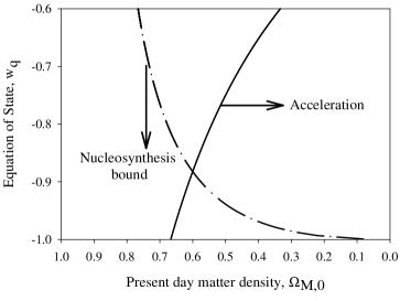
FIG. 1.: $\Omega_{M,0}$-$w_{q}$ parameter space for 3-way matter–kinetic–potential scaling solution with $\gamma=1$ and $\lambda<0$. Limits from nucleosynthesis constraints requiring $\tilde{\Omega}_{\psi,{\rm nuc}}^{\rm Max}=0.2$ are shown by a dot–dash line. The solid line shows the constraint from requiring acceleration at present.

IV Conclusions

We have presented the results of a phase-plane analysis of the evolution of spatially flat FRW cosmological models containing a barotropic fluid in a scalar-tensor theory of gravity where the Brans-Dicke scalar, $\propto\phi^{2}$, has a self-interaction potential, $V\propto\phi^{2n}$. In contrast to minimally coupled fields in general relativity, this scalar field has self-similar scaling solutions for an arbitrary power-law potential which correspond to fixed points in the phase-plane. The scalar-tensor gravity theory with perfect fluid in the Brans-Dicke frame, is equivalent to general relativistic gravity with an explicit interaction between the fluid and the scalar field in the conformally related Einstein frame. In this frame the effective potential for the scalar field is an exponential and the phase-plane coincides with that studied recently by Amendola [14], and Billyard and Coley [15].

There are five different possible fixed points for the system. Two of these are solutions where the scalar field’s kinetic energy dominates, and the fixed points coincide with O’Hanlon and Tupper’s vacuum solutions in Brans-Dicke theory [31]. A third solution, where the scalar field’s kinetic and potential energy remain proportional, coincides with Mathiazhagan and Johri’s [32] scalar-field dominated power-law solution, which is inflationary for $\lambda^{2}<2$. The fluid density is non-negligible only at the two remaining fixed points. When the self-interaction potential energy of the scalar field is negligible, we recover Nariai’s power-law solutions for a barotropic fluid in Brans-Dicke gravity. In these solutions, the rate of change of the Brans-Dicke field, and hence the effective gravitational constant $G\propto 1/\phi^{2}$, is inversely proportional to the Brans-Dicke parameter, $\omega$. But there is also a new solution when the scalar field kinetic and potential energy densities both remain proportional to the fluid density. In contrast to Nariai’s solutions, the rate of change of the effective gravitational constant is independent of the value of $\omega$ and depends only upon the potential exponent $n$. This 3-way scaling solution was originally discovered by in the context of Einstein gravity [17, 13].

We have investigated whether it is possible in this theoretical framework to construct cosmological solutions with non-relativistic (pressureless) matter which are accelerating at late cosmic times. A generalised dark matter model may be one way to achieve this, where non-relativistic dark matter is minimally coupled in a Brans-Dicke frame, but baryonic matter is minimally coupled in the conformally related Einstein frame (consistent with the current bounds on the variability of the gravitational constant [47]). This leads to an explicit energy transfer between the dark matter and the scalar field in the Einstein frame. In contrast to other scalar field models of quintessence [4, 48], scalar fields with potentials of pure exponential form, but non-minimally coupled to the dark matter, allow a late-time scaling solution with equation of state $w_{q}\approx-1$, as shown in Figure 1. It is only possible for the scalar field to make a significant contribution to the present energy density, while remaining consistent with nucleosynthesis limits upon the evolution during the radiation era, by approaching the strong coupling limit ($\omega_{\rm DM}\to-3/2$). Such strongly coupled dark matter is very different from the usual model of non-interacting dark matter and a more detailed investigation is necessary to determine whether this could represent a viable cosmological model .

Due to the scale-invariant nature of the theory and the existence of self-similar cosmological solutions, there is no fine-tuning required of the scalar field, either its initial conditions or its parameters, in order to produce a change to an accelerated expansion at late cosmic times. This can occur due to a change in the cosmological equation of state when a non-relativistic dark matter component, directly coupled to the scalar field, begins to make a significant contribution to the total density. This is a familiar feature of the standard hot big bang model where non-relativistic species, whether baryons or massive neutrinos or more exotic dark matter candidates, only come to affect the expansion at relatively late cosmic times.

Appendix: Eigenvalues of critical points

To determine the stability of solutions we expand about the critical points $(x_{i},y_{i})$,

$$x = x_{i}+u,$$ (A.1)

$$y = y_{i}+v$$ (A.2)

which to first order gives the equations of motion for $u$ and $v$,

$$u^{\prime} = \left(\frac{9}{2}(2-\gamma)x_{i}^{2}-2Wx_{i}-\frac{3}{2}\gamma y_{i}^{2}-\frac{3}{2}(2-\gamma)\right)u$$ (A.3)

$$+ \left((\lambda\sqrt{6}-3\gamma x_{i}-2W)y_{i}\right)v,$$ (A.4)

$$v^{\prime} = \left(3(2-\gamma)x_{i}y_{i}-\lambda\frac{3}{2}y_{i}\right)u$$ (A.5)

$$+ \left(\frac{3}{2}(2-\gamma)x_{i}^{2}-\lambda\frac{3}{2}x_{i}-\frac{9}{2}\gamma y_{i}^{2}+\frac{3}{2}\gamma\right)v.$$ (A.6)

We solve the simultaneous first order equations for two eigenvalues $m_{\pm}$ such that the eigenmodes $u=K_{\pm}v$ evolve as $u\propto e^{m_{\pm}N}$. Stability of the critical points $(x_{i},y_{i})$ depends on the eigenvalues $m_{\pm}$. Points are stable if the real part of the eigenvalues are negative, linear perturbations about the point being exponentially damped. A saddle point in the phase plane has the real part of the eigenvalues of opposite sign, whilst instability requires both real parts to be positive. The eigenvalues for the system are listed below.

In what follows we will make extensive use of the following bifurcation values for the parameters:

$$\gamma_{a} \equiv 2\left(1-{|W|\over 3}\right)\ ,$$ (A.7)

$$\lambda_{b} \equiv \sqrt{6}\ ,$$ (A.8)

$$\sqrt{6}\lambda_{c} \equiv 2W+{9\gamma(2-\gamma)\over 2W}\ ,$$ (A.9)

$$\sqrt{6}\lambda_{d\pm} \equiv W\pm\sqrt{W^{2}+18\gamma}\ .$$ (A.10)

1. 2–Way, Matter–Kinetic scaling solution

   $$m_{-} = -{3\over 2}\left[{(2-\gamma)^{2}-(2-\gamma_{a})^{2}\over(2-\gamma)}\right]\,,$$ (A.11)

   $$m_{+} = -\frac{2W(\lambda-\lambda_{c})}{\sqrt{6}(2-\gamma)}\,.$$ (A.12)

   Exists for $\gamma<\gamma_{a}$ and stable for $W(\lambda-\lambda_{c})>0$.

2. Kinetic dominated solutions $x=\pm 1,y=0$

   $$m_{+} = 3(2-\gamma)\mp 2W\,,$$ (A.13)

   $$m_{-} = 3\left(1\mp{\lambda\over\sqrt{6}}\right)\,,$$ (A.14)

   always exist. $x=\pm 1$ stable for $\pm W>0$, $\gamma>\gamma_{a}$ and $\pm\lambda>\lambda_{b}$.

3. Scalar field dominated solutions

   $$m_{+} = -{1\over 2}\left(6-\lambda^{2}\right)\,,$$ (A.15)

   $$m_{-} = (\lambda-\lambda_{d-})(\lambda-\lambda_{d+})$$ (A.16)

   Exists for $\lambda^{2}<\lambda_{b}^{2}$ and stable for $\lambda_{d-}<\lambda<\lambda_{d+}$.

4. 3–Way, Matter–Kinetic–Potential scaling solutions

   Eigenvalues, $m_{\pm}$ are defined by the solution to the quadratic equation,

   $$m^{2}+bm+c=0.$$ (A.17)

   where $b$ and $c$ are defined as,

   $$b=\frac{3}{(\sqrt{6}\lambda-2W)^{2}}[3(2-\gamma)(\lambda-\lambda_{d-})(\lambda-\lambda_{d+})$$ (A.18)

   $$\qquad-2W\sqrt{6}(\lambda-\lambda_{c})]\,,$$ (A.19)

   $$c=\frac{-6\sqrt{6}W(\lambda-\lambda_{d-})(\lambda-\lambda_{d+})(\lambda-\lambda_{c})}{(\sqrt{6}\lambda-2W)^{2}}\,,$$ (A.20)

   Exists for $W(\lambda_{c}-\lambda)>0$ and either $\lambda<\lambda_{d-}$ or $\lambda>\lambda_{d+}$. Always stable when it exists.

REFERENCES

- [1] N. Bahcall, J. P. Ostriker, S. Perlmutter and P. J. Steinhardt, Science 284, 1481 (1999) astro-ph/9906463.
- [2] M. Tegmark, Astrophys. J. 514, L69 (1999) astro-ph/9809201.
- [3] G. Efstathiou, S. L. Bridle, A. N. Lasenby, M. P. Hobson and R. S. Ellis, astro-ph/9812226.
- [4] I. Zlatev, L. Wang and P. J. Steinhardt, Phys. Rev. Lett. 82, 896 (1999) astro-ph/9807002; P. J. Steinhardt, L. Wang and I. Zlatev, Phys. Rev. D59, 123504 (1999) astro-ph/9812313.
- [5] C. Wetterich, Nucl. Phys. B302, 668 (1988).
- [6] E. J. Copeland, A. R. Liddle and D. Wands, Phys. Rev. D57, 4686 (1998) gr-qc/9711068.
- [7] A. R. Liddle and R. J. Scherrer, Phys. Rev. D59, 023509 (1999) astro-ph/9809272.
- [8] J. Wainwright and G. F. R. Ellis, “Dynamical Systems in Cosmology”, (C.U.P., Cambridge, 1997).
- [9] F. Lucchin and S. Matarrese, Phys. Rev. D32, 1316 (1985); Y. Kitada and K. Maeda, Class. Quant. Grav. 10, 703 (1993).
- [10] J. J. Halliwell, Phys. Lett. B185, 341 (1987).
- [11] A. B. Burd and J. D. Barrow, Nucl. Phys. B308, 929 (1988).
- [12] D. Wands, Cosmology of Scalar–Tensor Gravities, D.Phil. thesis, University of Sussex (1993).
- [13] C. Wetterich, Astron. Astrophys. 301, 321 (1995).
- [14] L. Amendola, Phys. Rev. D60 (1999) 043501, astro-ph/9904120.
- [15] A. P. Billyard and A. A. Coley, astro-ph/9908224.
- [16] A. P. Billyard, The Asymptotic Behaviour of Cosmological Models Containing Matter and Scalar Fields, Ph.D. thesis, Dalhousie University (1999) gr-qc/9908067.
- [17] D. Wands, E. J. Copeland and A. R. Liddle, Ann. N. Y. Acad. Sci. 688, 647 (1993).
- [18] C. H. Brans and R. H. Dicke, Phys. Rev. 124, 925 (1961).
- [19] J. E. Lidsey, D. Wands and E. J. Copeland, hep-th/9909061.
- [20] H. Nariai, Prog. Theor. Phys. 40, 49 (1968).
- [21] D. J. Holden and D. Wands, Class. Quantum Grav. 15, 3271 (1998) gr-qc/9803021.
- [22] B. Ratra and P. J. E. Peebles, Phys. Rev. D37, 3406 (1988); V. Sahni, H. Feldman and A. Stebbins, Astrophys. J. 385, 1 (1992).
- [23] R. R. Caldwell, R. Dave and P. J. Steinhardt, Phys. Rev. Lett. 80, 1582 (1998) astro-ph/9708069.
- [24] P. G. Bergmann, Int. J. Theor. Phys. 1, 25 (1968).
- [25] R. V. Wagoner, Phys. Rev. D1, 3209 (1970).
- [26] K. Nordtvedt, Astrophys. J. 161, 1059 (1970).
- [27] J. D. Barrow and K. Maeda, Nucl. Phys. B341, 294 (1990).
- [28] R. H. Dicke, Phys. Rev. 125, 2163 (1962).
- [29] M. B. Green, J. H. Schwarz and E. Witten, Superstring Theory (Cambridge University Press, Cambridge, 1988).
- [30] A.P. Billyard, A. Coley, J. Ibanez, Phys. Rev. D58 (1999) 023507
- [31] J. O’Hanlon and B. O. J. Tupper, Il Nuovo Cimento 7, 305 (1972).
- [32] C. Mathiazhagan and V. B. Johri, Class. Quantum Grav. 1, L29 (1984); D. La and P. J. Steinhardt, Phys. Rev. Lett. 62, 376 (1989).
- [33] C. Santos and R. Gregory, Annals Phys. 258, 111 (1997) gr-qc/9611065.
- [34] S. J. Kolitch, Annals Phys. 246, 121 (1996).
- [35] T. Damour and K. Nordtvedt, Phys. Rev. Lett. 70, 2217 (1993); Phys. Rev. D48, 3436 (1993).
- [36] C. Will, 1993 Theory and Experiment in Gravitational Physics (Cambridge University Press, Cambridge, 1993).
- [37] T. Damour, G.W. Gibbons, C. Gundlach, Phys. Rev. Lett. 64, 123 (1990).
- [38] J. A. Casas and J. García-Bellido, Class. Quantum Grav. 9, 1371 (1992) hep-ph/9204213.
- [39] P. G. Ferreira and M. Joyce, Phys. Rev. Lett. 79, 4740 (1997) astro-ph/9707286; Phys. Rev. D 58 023503 (1998) astro-ph/9711102.
- [40] S. Burles, K. M. Nollett, J. N. Truran and M. S. Turner, Phys. Rev. Lett. 82, 4176 (1999) astro-ph/9901157.
- [41] T. Damour and C. Gundlach, Phys. Rev. D 43, 3873 (1991).
- [42] J. A. Casas, J. García-Bellido and M. Quiros, Mod. Phys. Lett. A 7, 447 (1992).
- [43] M. S. Turner, to appear in The Third Stromlo Symposium: The Galactic Halo, eds. B. K. Gibson, T. S. Axelrod, and M. E. Putnam (Astron. Soc. Pac. Conf. Series, Vol. 666, 1999) astro-ph/9811454
- [44] W. L. Freedman, invited review ”Particle Physics and the universe”, Nobel Symposium, Haga Slott, Sweden, 1998, astro-ph/9905222.
- [45] P. M. Garnavich, et. al., Astron. J. 116, 1009 (1998) astro-ph/9806396.
- [46] S. Perlmutter, et. al., 1998, Astrophys. J. 517, 565 (1999) astro-ph/9812133.
- [47] D. B. Guenther, L. M. Krauss, P. Demarque, Astrophys. J. 498, 871 (1998).
- [48] G. Efstathiou, astro-ph/9904356.
- [49] L. Amendola, astro-ph/9908023.