(2+1)-dimensional Einstein-Kepler problem
in the centre-of-mass frame

Abstract

We formulate and analyse the Hamiltonian dynamics of a pair of massive spinless point particles in $(2+1)$-dimensional Einstein gravity by anchoring the system to a conical infinity, isometric to the infinity generated by a single massive but possibly spinning particle. The reduced phase space $\Gamma_{\rm red}$ has dimension four and topology ${\mathbb{R}}^{3}\times S^{1}$. $\Gamma_{\rm red}$ is analogous to the phase space of a Newtonian two-body system in the centre-of-mass frame, and we find on $\Gamma_{\rm red}$ a canonical chart that makes this analogue explicit and reduces to the Newtonian chart in the appropriate limit. Prospects for quantisation are commented on.

I Introduction

Einstein gravity in 2+1 spacetime dimensions provides an arena in which many of the conceptual features of $(3+1)$-dimensional Einstein gravity appear in a technically simplified setting [1]. One of these simplifications is that in 2+1 dimensions the theory can be consistently coupled to point particles. The spacetimes containing point particles can be described in terms of ${\rm IO}(2,1)$ holonomies around nontrivial loops [2, 3], and there exists considerable work on the global structure of these spacetimes [4, 5, 6, 7, 8, 9, 10, 11, 12, 13], much of it motivated by the observation that the spacetimes may contain closed causal curves. Several variational formulations of the dynamics have been introduced, both for examining the classical solution space in its own right and also as a starting point for quantisation [14, 15, 16, 17, 18, 19, 20, 21, 22, 23, 24].

In a spatially open universe, a variational formulation of Einstein gravity must specify boundary conditions at the infinity. In 3+1 dimensions, the spacelike infinity of an isolated system can be taken asymptotically Minkowski, and one can introduce in the Hamiltonian formulation a falloff that anchors the system to an asymptotic Minkowski spacetime [25, 26, 27]. The four-momentum and angular momentum of the system, defined as surface integrals at the infinity, can be interpreted respectively as a constant timelike vector and a constant spacelike vector in the asymptotic Minkowski spacetime, and the asymptotic Poincaré isometry group can be used to choose an asymptotic centre-of-mass Lorentz frame [25].

By contrast, in 2+1 dimensions the spacelike infinity of an isolated system is not asymptotically Minkowski but conical [28, 29]. The neighbourhood of the infinity has only two independent globally-defined Killing vectors, a timelike one generating time translations and a spacelike one generating rotations, but none that could be understood as generating boosts or spatial translations. It follows that the neighbourhood of the spacelike infinity contains information that defines an analogue of a centre-of-mass frame also in 2+1 dimensions: in the special case of a spacetime containing a single massive and possibly spinning point particle, the metric near the infinity uniquely determines the locus of the particle world line [2]. However, as the ${\rm IO}(2,1)$ holonomy around the infinity is nontrivial, with a nontrivial ${\rm O}(2,1)$ part, the ‘momentum’ and ‘angular momentum’ cannot be understood as constant vectors in an asymptotic $(2+1)$-dimensional Minkowski spacetime, and the analogue of the centre-of-mass frame cannot be realised as a Lorentz frame in an asymptotic Minkowski spacetime.

With point particle sources in a spatially open $(2+1)$-dimensional spacetime, there is thus a certain tension between two different viewpoints on the dynamics. On the one hand, one expects the conditions at the conical infinity to be crucial for defining what evolution means, for finding a Hamiltonian that generates this evolution, and for discussing symmetries and conservation laws. On the other hand, the relative motion of the particles takes a simple form when expressed in small patches of Minkowski geometry valid ‘between’ the particle world lines, but not valid globally, and in particular not valid in a neighbourhood of the infinity: this suggests formulating the dynamics first in terms of fields and variables that are defined locally, in small patches valid between the particles, and only later glueing the patches into a more globally-defined formulation that incorporates the conditions at the infinity. Each of the variational formulations of [14, 15, 16, 17, 18, 19, 20, 21, 22, 23, 24] strikes a different balance between these two viewpoints. An example near one extreme is [23], which specifies the trajectory of a single particle in terms of a reference point in the spacetime and a reference frame at this point. The purpose of the present paper is to approach the opposite extreme: we anchor the particle trajectories to the conical infinity at the very outset.

We concentrate on the case of two massive spinless particles, which can be regarded as the Kepler problem in $(2+1)$-dimensional Einstein gravity. Briefly put, we shall formulate and solve the Hamiltonian dynamics of the $(2+1)$-dimensional Einstein-Kepler problem in [the $(2+1)$-dimensional analogue of] the centre-of-mass frame.

To state the technical input more precisely, we assume the two-particle spacetime to have a spacelike infinity whose neighbourhood is isometric to a neighbourhood of the infinity in the spacetime of a single massive but possibly spinning point particle [2], with a defect angle less than $2\pi$. This is equivalent to assuming that the relative velocity of the two particles is less than the critical velocity found in [5, 6, 7], and it implies that the spacetime has no closed causal curves. The neighbourhood of the infinity admits a coordinate system that is adapted to the isometries, and these conical coordinates foliate the neighbourhood of the infinity by spacelike surfaces. We adopt these conical coordinates as the asymptotic structure to which the Hamiltonian dynamics will be anchored.

We take advantage of the well-known description of the two-particle spacetimes in terms of a piece of Minkowski geometry between the particle world lines [5, 6, 7, 8, 9, 10]. We first translate this description into one that relates the world lines of the particles to the conical infinity. We then use this explicit form of the classical solutions to reduce the first-order gravitational action, and we find on the reduced phase space a canonical chart analogous to that in a nongravitating two-particle system in the centre-of-mass frame. As expected from the nongravitating case, the reduced phase space has dimension four. The reduced Hamiltonian is bounded both above and below, in agreement with the general arguments of [28, 29], it has the correct relativistic test particle limit when the mass of one particle is small, and it has the correct nonrelativistic limit when the masses and velocities of both particles are small. The functional form of the Hamiltonian is nevertheless complicated, given only implicitly through the solution to a certain transcendental equation. Quantising this reduced Hamiltonian theory would thus seem to present a substantial challenge.

The plan of the paper is as follows. In section II we review the spacetime of a single spinning point particle and introduce the conical coordinates. Section III describes the two-particle spacetimes as anchored to the conical infinity. Section IV recalls the first-order action [23] of $(2+1)$-dimensional Einstein gravity coupled to massive point particles. The action is reduced in section V, and the reduced phase space is analysed in section VI. Section VII contains brief concluding remarks.

We use units in which $c=4\pi G=1$ (Planck’s constant will not appear). The Hamiltonian of a conical spacetime is in these units equal to half of the defect angle [23], and the mass of a point particle is then by definition half the defect angle at the particle world line. ${\rm O}_{\rm c}(2,1)$ and ${\rm IO}_{\rm c}(2,1)$ stand respectively for the connected components of ${\rm O}(2,1)$ and ${\rm IO}(2,1)$.

II Spacetime of a single spinning point particle

In this section we briefly review the spacetime of a single spinning point particle [2]. The main purpose is to establish the notation, in particular the conical coordinates (6).

Let $M$ be the $(2+1)$-dimensional spacetime obtained by removing a timelike geodesic from $(2+1)$ Minkowski space, and let ${\tilde{M}}$ be the universal covering space of $M$. We introduce on ${\tilde{M}}$ the global coordinates $(T,R,\theta)$ in which the metric reads

$$ds^{2}=-dT^{2}+dR^{2}+R^{2}d\theta^{2}\ \ ,$$ (1)

such that $R>0$, $-\infty<T<\infty$, and $-\infty<\theta<\infty$. The only linearly-independent globally-defined Killing vectors on ${\tilde{M}}$ are $\partial_{T}$ and $\partial_{\theta}$.

Consider on ${\tilde{M}}$ the isometry $J:=\exp\left(2\pi S\partial_{T}+2\pi\alpha\partial_{\theta}\right)$,

$$J:(T,R,\theta)\mapsto(T+2\pi S,R,\theta+2\pi\alpha)\ \ ,$$ (2)

where $\alpha>0$ and $S\in{\mathbb{R}}$. We interpret ${\tilde{M}}/J$ as the spacetime generated by a spinning point particle at $R=0$ [2]. The mass of the particle in our units is $\pi(1-\alpha)$, and we refer to $S$ as the spin. We take the mass to be positive, and we thus have $0<\alpha<1$.

${\tilde{M}}/J$ can be described in terms of a fundamental domain and an identification across its boundaries. As $\alpha<1$, this fundamental domain can be embedded in $M$, and the identification is then a $(2+1)$-dimensional Poincaré transformation, consisting of a $2\pi\alpha$ rotation about the removed timelike geodesic and a $2\pi S$ translation in the direction of this geodesic. One choice for the fundamental domain is the wedge $0<\theta<2\pi\alpha$.

We refer to $2\pi\alpha$ as the opening angle and to $\delta:=2\pi(1-\alpha)$ as the defect angle. When $S=0$, ${\tilde{M}}/J$ is the product spacetime of the time dimension and a two-dimensional cone, and this terminology conforms to the standard terminology for two-dimensional conical geometry.

We introduce on ${\tilde{M}}$ the coordinates $(t,R,\varphi)$ by

$$T=t+S\varphi\ \ ,$$ (4)

$$\theta=\alpha\varphi\ \ ,$$ (5)

so that $R>0$, $-\infty<T<\infty$, and $-\infty<\theta<\infty$, and the metric reads

$$ds^{2}=-(dt+Sd\varphi)^{2}+dR^{2}+\alpha^{2}R^{2}d\varphi^{2}\ \ .$$ (6)

In these coordinates $J=\exp(2\pi\partial_{\varphi})$, so that

$$J:(t,R,\varphi)\mapsto(t,R,\varphi+2\pi)\ \ .$$ (7)

With the usual abuse of terminology, we refer to $(t,R,\varphi)$ with the identification $(t,R,\varphi)\sim(t,R,\varphi+2\pi)$ as the conical coordinates on ${\tilde{M}}/J$. The only linearly-independent Killing vectors on ${\tilde{M}}/J$ are $\partial_{t}=\partial_{T}$ and $\partial_{\varphi}=\alpha\partial_{\theta}+S\partial_{T}$.

The conical coordinates on ${\tilde{M}}/J$ are uniquely defined up to the isometries generated by $\partial_{t}$ and $\partial_{\varphi}$. $\partial_{t}$ is timelike, while $\partial_{\varphi}$ is spacelike for $R>|S|/\alpha$, null for $R=|S|/\alpha$, and timelike for $R<|S|/\alpha$. One can think of $\partial_{t}$ as the generator of time translations and $\partial_{\varphi}$ as the generator of rotations. ${\tilde{M}}/J$ has closed causal curves, but none of them are contained in the region $R>|S|/\alpha$.

III Two-particle spacetimes with a conical infinity

In this section we describe the $(2+1)$-dimensional Einstein spacetimes with a pair of massive spinless point particles, assuming the spacelike infinity to be isometric to that of a single spinning point particle spacetime. In subsection III A we recall the well-known description in terms of a patch of Minkowski geometry between the particle world lines [5, 6, 7, 8, 9, 10]. In the remaining three subsections we translate this description into one in which the particle world lines are specified with respect to the conical infinity.

A Local description

We label the particles by the index $i=1,2$. If the spacetime contains a collision of the particles, we consider either the part outside the causal past of the collision or the part that is outside the causal future of the collision.

In a neighbourhood of the world line of each particle, the geometry is the spinless special case of the conical geometry of section II. The defect angles at the particles are $\delta_{i}:=2\pi(1-\alpha_{i})$. We regard these defect angles as prescribed parameters, and we write $c_{i}:=\cos(\delta_{i}/2)$, $s_{i}:=\sin(\delta_{i}/2)$. We take the masses of the particles to be positive, which implies $0<\delta_{i}<2\pi$, and the condition that the far-region geometry be conical implies $\delta_{1}+\delta_{2}<2\pi$ [7]. It follows that $s_{i}>0$ and $c_{1}+c_{2}>0$.

The description of the spacetime in terms of a sufficiently small piece $\tilde{D}$ of Minkowski spacetime ‘between’ the particles is well known [5, 6, 7, 8, 9, 10]. Each particle world line is a timelike geodesic on the boundary of $\tilde{D}$. The boundary segments of $\tilde{D}$ can in most cases be chosen as timelike plane segments joining at the particle world lines; the only exception is when the particle world lines are not in the same timelike plane in $\tilde{D}$ and one of the defect angles is greater than $\pi$, in which case the boundary segments need to be chosen suitably twisted (see subsection III D below). The identification across the two boundary segments joining at the world line of particle $i$ is a rotation about this world line by the angle $\delta_{i}$. The effect of encircling in the spacetime both particle world lines appears in the Minkowski geometry of $\tilde{D}$ as the composition of the two rotations, and this composition is a Poincaré transformation that may in general have a translational component as well as a Lorentz-component. Assuming the far-region geometry to be conical implies that the Lorentz-component is a rotation (and not a null rotation or a boost); this condition is equivalent to [7]

$$-1<c_{1}c_{2}-s_{1}s_{2}\cosh\beta\ \ ,$$ (8)

where $\beta$ denotes the relative boost parameter of the particle trajectories in $\tilde{D}$.

Our task is to translate this description into one anchored to the conical infinity. We proceed in the following steps:

$\bullet$ Cut $\tilde{D}$ into two along a suitably-chosen timelike surface connecting the particle world lines;

$\bullet$ Rotate the two halves of $\tilde{D}$ about the world line of particle $1$ so that the wedge originally at particle $1$ closes;

$\bullet$ In the resulting new fundamental domain, find a set of Minkowski coordinates $(T,X,Y)$ and cylindrical Minkowski coordinates $(T,R,\theta)$ in which the identification of the infinity-reaching boundary segments has the form (2);

$\bullet$ Introduce the conical coordinates $(t,R,\varphi)$ (II) in a neighbourhood of the infinity, extend this neighbourhood inward to the particle trajectories, and read off the particle trajectories in the conical coordinates.

When the particle trajectories are in the same timelike plane in the Minkowski geometry of $\tilde{D}$, the boundary segments of $\tilde{D}$ and the timelike surface along which $\tilde{D}$ is cut can each be chosen to be in a timelike plane, and implementing the above steps is relatively straightforward. However, when the particle trajectories in the Minkowski geometry of $\tilde{D}$ are not in the same timelike plane, the timelike surface along which $\tilde{D}$ is cut cannot be chosen to be in a plane, and when in addition one defect angle is larger than $\pi$, the boundary segments of $\tilde{D}$ cannot be chosen to be in timelike planes arbitrarily far into the future and the past (see subsection III D below). The geometry in this latter case is thus quite subtle.

We divide the analysis into three qualitatively different cases, proceeding from the simplest one to the most intricate one. First, when the particle trajectories in the Minkowski geometry of $\tilde{D}$ are parallel, the spacetime is static and has in particular vanishing spin. Second, when the particle trajectories in the Minkowski geometry of $\tilde{D}$ are in the same timelike plane but not parallel, the spacetime has a vanishing spin but is not static, and it contains a collision of the particles. Third, when the trajectories in the Minkowski geometry of $\tilde{D}$ are not in the same timelike plane, the spacetime has a nonvanishing spin: this is the ‘generic’ case. We devote a separate subsection to each case.

We record here the result, noted in [7] and to be verified below in all our three cases, that the defect angle $\delta$ of the far-region conical geometry is the unique solution in the interval $0<\delta<2\pi$ to the equation

$$\cos(\delta/2)=c_{1}c_{2}-s_{1}s_{2}\cosh\beta\ \ .$$ (9)

Note that this implies $\delta\geq\delta_{1}+\delta_{2}$, equality holding iff $\beta=0$. The parameter $\alpha$ of the far-region conical geometry is

$$\alpha=1-\delta/(2\pi)\ \ .$$ (10)

B $\beta=0$: Static spacetimes

When $\beta=0$, the particle world lines on the boundary of $\tilde{D}$ are parallel in the Minkowski geometry of $\tilde{D}$. We introduce in $\tilde{D}$ Minkowski coordinates $({\tilde{t}},{\tilde{x}},{\tilde{y}})$ such that $\partial_{\tilde{t}}$ points to the future, the world line of particle $1$ is $({\tilde{t}},{\tilde{x}},{\tilde{y}})=(\lambda,0,0)$, and the world line of particle $2$ is $({\tilde{t}},{\tilde{x}},{\tilde{y}})=(\lambda,-a,0)$, where $a$ is a positive constant. Here $\lambda$ stands for a proper time parameter individually on each world line.

We choose $\tilde{D}$ so that its boundary segments are half-planes bounded by the particle world lines and its intersection with the surface ${\tilde{t}}=0$ is as shown in figure 1. The spacetime is clearly static.

To obtain an equivalent fundamental domain that is better adapted to the infinity, we proceed as outlined in subsection III A. We first work in the plane of figure 1 and then extend into the time dimension by staticity.

We cut the planar fundamental domain of figure 1 into two along the straight line connecting the particles, and we rotate the two halves with respect to each other about particle $1$ so that the wedge on the right closes. The new planar fundamental domain is shown in figure 2: the corner labelled $1$ is at the first particle, while the corners labelled $2$ and $2^{\prime}$ are both at the second particle. We introduce in this new planar fundamental domain polar coordinates $(R,\theta)$ in which the boundary segments from $2$ and $2^{\prime}$ to infinity are at constant $\theta$: the origin of these polar coordinates lies outside the domain and is labelled in figure 2 by $O$. We denote the value of $R$ at corner $1$ by $R_{1}$, and that at corners $2$ and $2^{\prime}$ by $R_{2}$. Elementary planar geometry yields

$$R_{1}=\frac{as_{2}}{\sin(\delta/2)}\ \ ,$$ (12)

$$R_{2}=\frac{as_{1}}{\sin(\delta/2)}\ \ ,$$ (13)

where $\delta=\delta_{1}+\delta_{2}$. Choosing the corner $1$ to be at $\theta=0$, the corners $2$ and $2^{\prime}$ are respectively at $\theta=\pm(\pi-\delta/2)$.

The new spacetime fundamental domain $D$ is the product of the planar fundamental domain of figure 2 and the time axis. In the cylindrical Minkowski coordinates $(T,R,\theta)$ (1) in $D$, the two infinity-reaching boundary segments of $D$ are in the half-planes $\theta=\pm(\pi-\delta/2)$, and their identification is a pure rotation about the (fictitious) axis at $R=0$. A spacetime picture of $D$ is shown in figure 3. The spacetime near the infinity is thus conical with vanishing spin, and $\delta$ is the defect angle. Note that this discussion verifies equation (9) in the special case $\beta=0$.

We now introduce near the infinity the conical coordinates $(t,R,\varphi)$ as in (II), with $S=0$ and with $\alpha$ given by (10), except in that we add to $\varphi$ a constant $-\varphi_{0}$ that is defined modulo $2\pi$. The conical coordinates are valid in a neighbourhood of the infinity, and we can extend this neighbourhood inwards (in a $\varphi$-dependent way if $\delta_{1}\neq\delta_{2}$) so that the boundary of the extended neighbourhood contains the trajectories of both particles. The world line of particle 1 is then at $(t,R,\varphi)=(\lambda,R_{1},\varphi_{0})$, and that of particle 2 is at $(t,R,\varphi)=(\lambda,R_{2},\varphi_{0}+\pi)$.

To summarise, we have introduced a neighbourhood of the infinity covered by the conical coordinates $(t,R,\varphi)$ and expressed the particle trajectories as lines on the boundary of this neighbourhood. The values of the radial coordinate $R$ at the particles are given by (III B), and the values of the angular coordinate $\varphi$ are respectively $\varphi_{0}$ and $\varphi_{0}+\pi$: in this sense, the particles are diametrically opposite each other. The parameter $\varphi_{0}$ specifies the orientation of the two-particle system relative to the conical coordinates, and spacetimes differing only in the value of $\varphi_{0}$ are clearly isometric.

C $\beta\neq 0$, $S=0$: Spacetimes with colliding particles

When $\beta\neq 0$ but the particle trajectories in the Minkowski geometry of $\tilde{D}$ are in the same timelike plane, the spacetime contains a collision of the particles. We consider either the part outside the causal past of the collision or the part that is outside the causal future of the collision.

As in subsection III B, we introduce in $\tilde{D}$ Minkowski coordinates $({\tilde{t}},{\tilde{x}},{\tilde{y}})$ in which the world line of particle $1$ is $({\tilde{t}},{\tilde{x}},{\tilde{y}})=(\lambda,0,0)$. We now choose these coordinates so that the world line of particle $2$ is $({\tilde{t}},{\tilde{x}},{\tilde{y}})=(\lambda\cosh\beta,-\lambda\sinh\beta,0)$ at ${\tilde{x}}<0$. The particles collide at $({\tilde{t}},{\tilde{x}},{\tilde{y}})=(0,0,0)$. For $\beta>0$ ($\beta<0$, respectively), the particles are receding (approaching).

We choose $\tilde{D}$ so that its intersection with the surface ${\tilde{t}}=0$ is as shown in figure 4. The boundary segments of $\tilde{D}$ are continued to ${\tilde{t}}\neq 0$ in the half-planes bounded by the respective particle world lines.

To find a fundamental domain better suited to the infinity, we proceed as outlined in subsection III A. We cut $\tilde{D}$ into two along the totally geodesic timelike surface between the particle world lines, and we rotate the two halves with respect to each other about the world line of particle $1$ so that the wedge originally at particle $1$ closes. In the resulting new fundamental domain $D$, we introduce Minkowski coordinates $(T,X,Y)$ and cylindrical Minkowski coordinates $(T,R,\theta)$ in which the identification of the infinity-reaching boundary segments has the form (2). We choose these coordinates so that particle $1$ has always $\theta=0$ and the collision of the particles is at $(T,X,Y)=(0,0,0)$.

The algebra in finding $(T,R,\theta)$ is lengthy but straightforward. A constant $T$ surface of $D$ is shown in figure 5, with $T>0$ ($T<0$) for $\beta>0$ ($\beta<0$). The first particle is at the corner labelled $1$, at $(T,R,\theta)=(T,T\tanh\beta_{1},0)$, and the second particle is at the corners labelled $2$ and $2^{\prime}$, respectively at $(T,R,\theta)=\biglb(T,T\tanh\beta_{2},\pm(\pi-\delta/2)\bigrb)$, where $\delta$ is defined by (9) and $\beta_{i}$ by

$$\sinh\beta_{1}=\frac{s_{2}\sinh\beta}{\sin(\delta/2)}\ \ ,$$ (15)

$$\sinh\beta_{2}=\frac{s_{1}\sinh\beta}{\sin(\delta/2)}\ \ .$$ (16)

$\beta_{i}$ are thus the boost parameters of the particle world lines with respect to the coordinates $(T,X,Y)$. The boundary of $D$ between edges $1$ and $2$ is the timelike plane sector connecting these edges, and similarly for the boundary between edges $1$ and $2^{\prime}$. The infinity-reaching boundaries are in the timelike planes $\theta=\pm(\pi-\delta/2)$, and their identification is by the map (2) with $S=0$. The spacetime near the infinity is thus conical with $S=0$, and the defect angle is $\delta$. A spacetime picture of $D$ (with $\beta>0$) is shown in figure 6.

Near the infinity, we introduce conical coordinates $(t,R,\varphi)$ as in (II), except in that we replace $t$ by $t-t_{0}$ and $\varphi$ by $\varphi-\varphi_{0}$, where $t_{0}$ and $\varphi_{0}$ are constants, the latter one defined modulo $2\pi$. The resulting conical coordinates are valid in a neighbourhood of infinity, and we extend this neighbourhood inwards so that the particle trajectories lie on its boundary. The trajectory of particle $1$ is $(t,R,\varphi)=(t_{0}+\lambda\cosh\beta_{1},\lambda\sinh\beta_{1},\varphi_{0})$, and that of particle $2$ is $(t,R,\varphi)=(t_{0}+\lambda\cosh\beta_{2},\lambda\sinh\beta_{2},\varphi_{0}+\pi)$. The particles are thus again diametrically opposite at each $t$, and the constant $\varphi_{0}$ is the conical angle of particle $1$, specifying the orientation of the two-particle system with respect to the infinity. The constant $t_{0}$ is the value of the conical time at the collision of the particles.

D $S\neq 0$: Spinning spacetimes

When the particle trajectories in the Minkowski geometry of $\tilde{D}$ are not in the same timelike plane, we again introduce in $\tilde{D}$ Minkowski coordinates $({\tilde{t}},{\tilde{x}},{\tilde{y}})$ such that $\partial_{\tilde{t}}$ points to the future and the world line of particle $1$ is $({\tilde{t}},{\tilde{x}},{\tilde{y}})=(\lambda,0,0)$. We now choose the coordinates so that the world line of particle $2$ is $({\tilde{t}},{\tilde{x}},{\tilde{y}})=(\lambda\cosh\beta,-a,-\lambda\sinh\beta)$, where $a>0$ and $\beta\neq 0$.

We choose the intersection of $\tilde{D}$ with the surface ${\tilde{t}}=0$ as shown in figure 7. If neither defect angle is greater than $\pi$, one possible choice for the boundary segments of $\tilde{D}$ would be to continue them off the ${\tilde{t}}=0$ surface as timelike half-planes bounded by the respective particle world lines [5, 10]. If one defect angle is greater than $\pi$, such half-planes would however eventually intersect the trajectory of the other particle, and the boundary segments need to be chosen suitably twisted. It is fortunately not necessary to specify here precisely how the boundary segments of $\tilde{D}$ are chosen: we shall construct a new fundamental domain $D$ as outlined in subsection III A, and we shall specify the boundary segments of $D$ in a way that is more easily described directly in terms of $D$. In particular, we choose the infinity-reaching boundary segments of $D$ not to be in timelike planes for any values of the defect angles.

We first choose in $\tilde{D}$ a timelike surface that connects the world lines of the two particles. We take this surface to contain the spacelike geodesic that connects the particles at ${\tilde{t}}=0$, shown as the dashed line in figure 7; the choice of the surface for ${\tilde{t}}\neq 0$ will be specified shortly. We cut $\tilde{D}$ into two along this surface, and we rotate the two halves with respect to each other about the world line of particle $1$ so that the wedge originally at particle $1$, in figure 7 on the right, closes. The ${\tilde{t}}=0$ surface of the resulting domain $D$ is shown in figure 8. The corner labelled $1$ is at the first particle, and the corners labelled $2$ and $2^{\prime}$ are both at the second particle.

Finding in $D$ Minkowski coordinates $(T,X,Y)$ and cylindrical Minkowski coordinates $(T,R,\theta)$ in which the identification of the infinity-reaching boundary segments has the form (2) is again lengthy but straightforward. Let $\delta$ be defined by (9), let $\beta_{i}$ be defined by (III C), and let

$$\rho_{1}:=\frac{as_{2}\cosh\beta_{2}}{\sin(\delta/2)}\ \ ,$$ (18)

$$\rho_{2}:=\frac{as_{1}\cosh\beta_{1}}{\sin(\delta/2)}\ \ .$$ (19)

Let $(T_{1},R_{1},\theta_{1})$ stand for the cylindrical Minkowski coordinates of the edge labelled $1$ in figure 8, and let $(T_{2},R_{2},\theta_{2})$ and $(T_{2^{\prime}},R_{2^{\prime}},\theta_{2^{\prime}})$ similarly stand for the respective cylindrical Minkowski coordinates of the edges labelled $2$ and $2^{\prime}$. We choose the point ${\tilde{t}}=0$ at edge $1$ to be at $T_{1}=0=\theta_{1}$. We then find

$$R_{1} = \frac{\rho_{1}}{\cos\sigma}\ \ ,$$ (21)

$$R_{2}=R_{2^{\prime}} = \frac{\rho_{2}}{\cos\sigma}\ \ ,$$ (22)

$$T_{1}=\frac{a\cosh\beta_{1}\cosh\beta_{2}}{\sinh\beta}\tan\sigma\ \ ,$$ (24)

$$T_{2}=a\left[\frac{\cosh\beta_{1}\cosh\beta_{2}}{\sinh\beta}\tan\sigma+\frac{s_{1}s_{2}\sinh\beta}{\sin(\delta/2)}\right]\ \ ,$$ (25)

$$T_{2^{\prime}}=a\left[\frac{\cosh\beta_{1}\cosh\beta_{2}}{\sinh\beta}\tan\sigma-\frac{s_{1}s_{2}\sinh\beta}{\sin(\delta/2)}\right]\ \ ,$$ (26)

and

$$\theta_{1}=\sigma\ \ ,$$ (28)

$$\theta_{2}=\sigma+\alpha\pi\ \ ,$$ (29)

$$\theta_{2^{\prime}}=\sigma-\alpha\pi\ \ ,$$ (30)

where $\sigma\in(-{\frac{1}{2}}\pi,{\frac{1}{2}}\pi)$ is a parameter along each of the three edges. For $\beta>0$ ($\beta<0$), $\sigma$ grows towards the future (past). The map that identifies the infinity-reaching boundary segments of $D$, taking in particular edge $2^{\prime}$ to edge $2$, is (2) with

$$S:=\frac{as_{1}s_{2}\sinh\beta}{\pi\sin(\delta/2)}\ \ .$$ (31)

In the Minkowski coordinates $(T,X,Y)$, the tangent vector of edge $1$ is $(\cosh\beta_{1},\sinh\beta_{1},0)$, the tangent vector of edge $2$ is $\biglb(\cosh\beta_{2},-\sinh\beta_{2}\sin(\delta/2),-\sinh\beta_{2}\cos(\delta/2)\bigrb)$, and the tangent vector of edge $2^{\prime}$ is $\biglb(\cosh\beta_{2},\sinh\beta_{2}\sin(\delta/2),-\sinh\beta_{2}\cos(\delta/2)\bigrb)$. $\beta_{i}$ are thus the boost parameters of the respective edges with respect to the coordinates $(T,X,Y)$, as in the colliding-particle spacetimes of subsection III C.

Having found the edges on the boundary of $D$, we are ready to specify the rest of the boundary. First, note that the identification of edges $2$ and $2^{\prime}$ takes a point on edge $2^{\prime}$ with a given value of $\sigma$ to a point on edge $2$ with the same value of $\sigma$. We can therefore choose the boundary segment between edges $1$ and $2$ to consist of geodesics joining edge $1$ to edge $2$ at the same value of $\sigma$ on the two edges, and similarly for the boundary segment between edges $1$ and $2^{\prime}$: this specifies the way how $\tilde{D}$ was cut in two. All these geodesics are spacelike. Finally, we take the boundary segment from edge $2$ to infinity to consist of half-lines at constant $T$ and $\theta$, and similarly for the boundary segment from edge $2^{\prime}$ to infinity.

Figure 9 shows the $\sigma=0$ configuration of $D$ in the the Minkowski coordinates $(T,X,Y)$, with the $T$-coordinate suppressed: the plane of the paper is at $T=0$ and corner $1$ is in this plane, while corner $2$ is above and corner $2^{\prime}$ is below this plane for $\beta>0$, and conversely for $\beta<0$. Figure 10 shows the configuration at a larger value of $\sigma$, with the $T$-coordinate similarly suppressed: this configuration is later (earlier) for $\beta>0$ ($\beta<0$). A spacetime picture of $D$ is shown in figure 11 (for $\beta>0$). Note how all the boundary segments of $D$ twist as the particles evolve in $T$: none of these segments is in a timelike plane.

Near the infinity, we introduce conical coordinates $(t,R,\varphi)$ as in subsection III C, replacing in the transformation (II) $t$ by $t-t_{0}$ and $\varphi$ by $\varphi-\varphi_{0}$, and we extend the neighbourhood of the infinity inwards to the particle world lines. In terms of the parameter $\sigma$, the particle trajectories in the conical coordinates are then given by (III D) with

$$\varphi_{1}=\varphi_{0}+\sigma/\alpha\ \ ,$$ (33)

$$\varphi_{2}=\varphi_{0}+\sigma/\alpha+\pi\ \ ,$$ (34)

$$t_{1}=t_{2}=t_{0}+a\left[\frac{\cosh\beta_{1}\cosh\beta_{2}}{\sinh\beta}\tan\sigma-\frac{s_{1}s_{2}\sinh\beta}{\pi\alpha\sin(\delta/2)}\sigma\right]\ \ .$$ (35)

The particles at a given $\sigma$ are thus on the same constant $t$ surface. Equation (35) can be uniquely inverted for $\sigma$ as a function of $t\in(-\infty,\infty)$, and the resulting function $\sigma(t)$ vanishes at $t=t_{0}$. Substituting this $\sigma(t)$ in (III D) and (III D) yields the particle trajectories in the form $\biglb(t,R_{i}(t),\varphi_{i}(t)\bigrb)$.

Equations (III D) show that the particle world lines intersect a constant $t$ surface at values of $\varphi$ that differ by $\pi$. In this sense, the particles are at each $t$ again diametrically opposite each other. To understand geometrically the constants $t_{0}$ and $\varphi_{0}$, we observe that the length of the geodesic connecting the particles at a given $t$ is

$$R_{c}:=\frac{a}{\cos\sigma}\sqrt{1+\frac{s_{1}^{2}s_{2}^{2}\sinh^{2}\beta\sin^{2}\sigma}{\sin^{2}(\delta/2)}}\ \ ,$$ (36)

which reaches its minimum at $\sigma=0$, or in other words at $t=t_{0}$, at which moment $\varphi_{1}=\varphi_{0}$. $t_{0}$ is therefore the moment of conical time at which the particles are at their smallest spatial separation, and $\varphi_{0}$ is the conical angle of particle $1$ at this moment. The constants $t_{0}$ and $\varphi_{0}$ thus encode the zero-point of time and the orientation of the two-particle system relative to the conical coordinates.

It follows from the general considerations of [5, 6, 7] that the spacetime does not have closed causal curves. In particular, it can be verified that $\rho_{i}$ are larger than the critical radius $|S|/\alpha$ at which closed causal curves appear in the spacetime of a single spinning particle.

Finally, note that the static spacetimes of subsection III B can be obtained from the spinning spacetimes in the limit $\beta\to 0$. The correct limiting forms for formulas involving the parameter $\sigma$ (which becomes ill-defined in the limit) arise after first replacing $\sigma$ by the new parameter $\lambda:=a\sigma/\beta$, which always increases toward the future. Similarly, the colliding-particle spacetimes of subsection III C can be obtained from the spinning spacetimes in the limit $a\to 0$ with fixed $\beta\neq 0$, provided one first restricts $t-t_{0}$ to having only one sign, positive (negative) values yielding a spacetime to the future (past) of the collision. If the sign of $t-t_{0}$ is unrestricted, the limit $a\to 0$ with fixed $\beta\neq 0$ is ambiguous: the reason is that for $S\neq 0$, the particles scatter off each other so that each conical angle changes from the asymptotic past to the asymptotic future by $(\pi/\alpha)\,{\rm sgn}(\beta)$, and the $a\to 0$ limit of this quantity with fixed $\beta\neq 0$ depends on the sign of $\beta$. Constructing a colliding-particle spacetime that contains both the past and the future of the collision requires thus additional assumptions: an example is the elastic collision discussed in [13].

IV Action in the connection formulation

In this section we recall a first-order formulation of 2+1 gravity [30, 31, 32, 33] with massive point particles [23]. We follow the notation of [32, 33, 34], with the exception that we use units in which $4\pi G=1$ [23].

A Bulk action

The $(2+1)$-dimensional gravitational field in the connection formulation is a connection in an ${\rm IO}_{\rm c}(2,1)$ bundle over the three-dimensional spacetime manifold. With our spacetime topology the relevant bundle is the trivial one, and we can without loss of generality work in a global trivialisation. The gravitational field can then be written as the globally-defined ${\rm O}_{\rm c}(2,1)$ connection one-form ${\bar{A}}_{a}^{I}$, taking values in the Lie algebra ${\mathfrak{o}}(2,1)\simeq{\mathfrak{s}l}(2,{\mathbb{R}})$, and the globally-defined co-triad ${\bar{e}}_{aI}$ one-form, taking values in the dual of this Lie algebra. The internal indices $I,J,\ldots$ take values in $\left\{0,1,2\right\}$, and they are raised and lowered with the internal Minkowski metric, $\eta_{IJ}={\rm{diag}}(-1,1,1)$. The indices $a,b,\ldots$ are abstract spacetime indices.

The bulk action reads

$$S=\frac{1}{4}\int_{M}{d^{3}x}\,\tilde{\eta}^{abc}\,{\bar{e}}_{aI}{\bar{F}}^{I}_{bc}\ \ ,$$ (37)

where $\tilde{\eta}^{abc}$ is the Levi-Civita density and ${\bar{F}}^{I}_{bc}$ is the curvature of the connection,

$${\bar{F}}^{I}_{bc}=2\partial^{\phantom{I}}_{[b}{\bar{A}}^{I}_{c]}+\epsilon^{I}{}_{JK}{\bar{A}}^{J}_{b}{\bar{A}}^{K}_{c}\ \ .$$ (38)

The structure constants $\epsilon^{I}{}_{JK}$ are obtained from the totally antisymmetric symbol $\epsilon_{IJK}$ by raising the index with the Minkowski metric. Our convention is $\epsilon_{012}=1$. When the co-triad is nondegenerate, the metric ${\bar{e}}_{aI}{\bar{e}}_{b}^{I}$ has signature $(-,+,+)$, and the field equations derived from (37) imply flatness of the metric, which is equivalent to the metric’s satisfying the vacuum Einstein equations.

Changing the global trivialisation of the ${\rm IO}_{\rm c}(2,1)$ bundle gives rise to the gauge transformation

$${\bar{A}}^{I}_{a}K_{I} \mapsto {\left({\sf R}^{-1}\right)}^{I}{\vphantom{\left({\sf R}^{-1}\right)}}_{J}\,{\bar{A}}^{J}_{a}K_{I}+{\sf R}^{-1}\partial_{a}{\sf R}\ \ ,$$ (40)

$${\bar{e}}^{I}_{a} \mapsto {\left({\sf R}^{-1}\right)}^{I}{\vphantom{\left({\sf R}^{-1}\right)}}_{J}\left({\bar{e}}^{J}_{a}+{\bar{\cal D}}_{a}w^{J}\right)\ \ ,$$ (41)

where the matrix ${\sf R}$ takes values in the defining representation of ${\rm O}_{\rm c}(2,1)$, ${\bar{\cal D}}_{a}$ is the gauge-covariant derivative determined by ${\bar{A}}^{I}_{a}$,

$${\bar{\cal D}}_{a}v_{K}=\partial_{a}v_{K}-\epsilon^{I}{}_{JK}{\bar{A}}^{J}_{a}v_{I}\ \ ,$$ (42)

and $K_{I}$ are the ${\mathfrak{o}}(2,1)$ adjoint representation basis matrices with the components ${\left(K_{J}\right)}^{I}{\vphantom{\left(K_{I}\right)}}_{L}=\epsilon^{I}{}_{JL}$,

$$K_{0}=\pmatrix{0&0&0\cr 0&0&-1\cr 0&1&0\cr}\ \ ,\ \ K_{1}=\pmatrix{0&0&-1\cr 0&0&0\cr-1&0&0\cr}\ \ ,\ \ K_{2}=\pmatrix{0&1&0\cr 1&0&0\cr 0&0&0\cr}\ \ .$$ (43)

We recall for future use the identities

$${\sf R}K_{I}{\sf R}^{-1}={{\sf R}}^{J}{\vphantom{{\sf R}}}_{I}\,K_{J}\ \ ,$$ (45)

$${\rm Tr}(K_{I}K_{J})=2\eta_{IJ}\ \ .$$ (46)

If the transformation (IV A) is connected to the identity, it leaves the action (37) invariant. If the transformation is not connected to the identity, the action (37) may acquire a topological additive constant.

We now take the spacetime manifold to be ${\mathbb{R}}\times\Sigma$, where $\Sigma$ is the plane with two punctures. The 2+1 decomposition of the bulk action reads [31, 32, 33]

$$S_{\rm bulk}={\frac{1}{2}}\int dt\int_{\Sigma}d^{2}x\left[{\tilde{E}}^{j}_{I}\left(\partial_{t}A^{I}_{j}\right)+{\bar{A}}^{I}_{t}{\cal D}_{j}{\tilde{E}}^{j}_{I}+{\frac{1}{2}}{\bar{e}}_{tI}F^{I}_{ij}{\tilde{\eta}}^{ij}\right]\ \ .$$ (47)

The abstract indices $i,j,\ldots$ live on $\Sigma$, and $t$ is the coordinate on ${\mathbb{R}}$. The ${\rm O}_{\rm c}(2,1)$ connection $A^{I}_{j}$ is the pull-back of ${\bar{A}}_{a}^{I}$ to $\Sigma$, $F^{I}_{ij}$ is its curvature, given by

$$F^{I}_{ij}=2\partial^{\phantom{I}}_{[i}A^{I}_{j]}+\epsilon^{I}{}_{JK}A^{J}_{i}A^{K}_{j}\ \ ,$$ (48)

and ${\tilde{\eta}}^{ij}$ is the Levi-Civita density on $\Sigma$. The vector density ${\tilde{E}}^{j}_{I}$ is given by ${\tilde{E}}^{j}_{I}={\tilde{\eta}}^{ji}e_{iI}$, where $e_{iI}$ is the pull-back of ${\bar{e}}_{aI}$ to $\Sigma$. ${\cal D}_{j}$ is the gauge-covariant derivative on $\Sigma$ determined by $A^{I}_{j}$,

$${\cal D}_{j}v_{K}=\partial_{j}v_{K}-\epsilon^{I}{}_{JK}A^{J}_{j}v_{I}\ \ .$$ (49)

The canonical pair is thus $(A^{I}_{j},{\tilde{E}}^{j}_{I})$, and the Poisson brackets read

$$\left\{A^{I}_{i}(x),{\tilde{E}}^{j}_{J}(x^{\prime})\right\}=2\,\delta^{j}_{i}\delta^{I}_{J}\delta\left(x,x^{\prime}\right)\ \ ,$$ (50)

where $x$ and $x^{\prime}$ denote points on $\Sigma$. ${\bar{e}}_{tI}$ and ${\bar{A}}^{I}_{t}$ act as Lagrange multipliers enforcing the constraints

$$F^{I}_{ij} = 0$$ (52)

$${\cal D}_{j}{\tilde{E}}^{j}_{I} = 0\ \ .$$ (53)

B Boundary conditions and boundary terms

We now turn to the boundary conditions. From now on we assume that the co-triad ${\bar{e}}_{aI}$ is nondegenerate everywhere on $\Sigma$. We write ${\mathchoice{{\hbox{\boldmath$\displaystyle\bar{A}$}}}{{\hbox{\boldmath$\textstyle\bar{A}$}}}{{\hbox{\boldmath$\scriptstyle\bar{A}$}}}{{\hbox{\boldmath$\scriptscriptstyle\bar{A}$}}}}^{I}:={\bar{A}}_{a}^{I}dx^{a}$, ${\mathchoice{{\hbox{\boldmath$\displaystyle\bar{e}$}}}{{\hbox{\boldmath$\textstyle\bar{e}$}}}{{\hbox{\boldmath$\scriptstyle\bar{e}$}}}{{\hbox{\boldmath$\scriptscriptstyle\bar{e}$}}}}^{I}:={\bar{e}}_{a}^{I}dx^{a}$, ${\mathchoice{{\hbox{\boldmath$\displaystyle A$}}}{{\hbox{\boldmath$\textstyle A$}}}{{\hbox{\boldmath$\scriptstyle A$}}}{{\hbox{\boldmath$\scriptscriptstyle A$}}}}^{I}:={A}_{j}^{I}dx^{j}$, ${\mathchoice{{\hbox{\boldmath$\displaystyle e$}}}{{\hbox{\boldmath$\textstyle e$}}}{{\hbox{\boldmath$\scriptstyle e$}}}{{\hbox{\boldmath$\scriptscriptstyle e$}}}}^{I}:={e}_{j}^{I}dx^{j}$.

Near the infinity, we introduce on $\Sigma$ polar coordinates $(r,\varphi)$, identified as $(r,\varphi)\sim(r,\varphi+2\pi)$, such that the infinity is at $r\to\infty$. We assume that in some neighbourhood of the infinity the variables take the form

$${\mathchoice{{\hbox{\boldmath$\displaystyle\bar{e}$}}}{{\hbox{\boldmath$\textstyle\bar{e}$}}}{{\hbox{\boldmath$\scriptstyle\bar{e}$}}}{{\hbox{\boldmath$\scriptscriptstyle\bar{e}$}}}}^{0} = dt+Sd\varphi\ \ ,$$ (55)

$${\mathchoice{{\hbox{\boldmath$\displaystyle\bar{e}$}}}{{\hbox{\boldmath$\textstyle\bar{e}$}}}{{\hbox{\boldmath$\scriptstyle\bar{e}$}}}{{\hbox{\boldmath$\scriptscriptstyle\bar{e}$}}}}^{1} = dr\ \ ,$$ (56)

$${\mathchoice{{\hbox{\boldmath$\displaystyle\bar{e}$}}}{{\hbox{\boldmath$\textstyle\bar{e}$}}}{{\hbox{\boldmath$\scriptstyle\bar{e}$}}}{{\hbox{\boldmath$\scriptscriptstyle\bar{e}$}}}}^{2} = \alpha rd\varphi\ \ ,$$ (57)

$${\mathchoice{{\hbox{\boldmath$\displaystyle\bar{A}$}}}{{\hbox{\boldmath$\textstyle\bar{A}$}}}{{\hbox{\boldmath$\scriptstyle\bar{A}$}}}{{\hbox{\boldmath$\scriptscriptstyle\bar{A}$}}}}^{0} = \alpha d\varphi\ \ ,$$ (58)

$${\mathchoice{{\hbox{\boldmath$\displaystyle\bar{A}$}}}{{\hbox{\boldmath$\textstyle\bar{A}$}}}{{\hbox{\boldmath$\scriptstyle\bar{A}$}}}{{\hbox{\boldmath$\scriptscriptstyle\bar{A}$}}}}^{1} = {\mathchoice{{\hbox{\boldmath$\displaystyle\bar{A}$}}}{{\hbox{\boldmath$\textstyle\bar{A}$}}}{{\hbox{\boldmath$\scriptstyle\bar{A}$}}}{{\hbox{\boldmath$\scriptscriptstyle\bar{A}$}}}}^{2}=0\ \ ,$$ (59)

where $\alpha$ and $S$ may depend on $t$, and they satisfy $\alpha>0$, $-\infty<S<\infty$. The integral defining $S_{\rm bulk}$ is then convergent at the infinity (since the integrand in (47) vanishes when (IV B) holds), and the variation of $S_{\rm bulk}$ acquires from the infinity the boundary term $-\pi\int dt\,\delta\alpha$. This boundary term is cancelled provided we add to $S_{\rm bulk}$ the infinity boundary action

$$S_{\infty}:=\pi\int dt\,(\alpha-1)\ \ .$$ (60)

The constant term in the integrand in (60) has been chosen for later convenience.

The field equations for the ansatz (IV B) are equivalent to the $t$-independence of $\alpha$ and $S$. When $\alpha$ and $S$ are $t$-independent, the metric obtained from (IV B) is the conical metric of section II, and $(t,r,\varphi)$ are a set of conical coordinates. The infinity behavior (IV B) and the boundary action (60) therefore reproduce the desired classical solutions near the infinity.

Consider then the particles, which we label by the index $i=1,2$ as in section III. We denote the masses by $m_{i}$, we regard these masses as prescribed parameters, and we assume $0<m_{i}<\pi$, $0<m_{1}+m_{2}<\pi$. Near each particle, we introduce on $\Sigma$ local polar coordinates $(r,\varphi)$, identified as $(r,\varphi)\sim(r,\varphi+2\pi)$, such that the particle is at the puncture of $\Sigma$ at $r\to 0_{+}$. (We suppress on these coordinates the index pertaining to the particle.) The boundary actions at the particles read [23], in our notation,

$$S_{i}:={\frac{1}{2}}\int dt\int_{r=0}d\varphi\,{\bar{A}}^{I}_{t}e_{I\varphi}-\int dt\,\zeta_{i}\left[{\frac{1}{2}}{\rm Tr}(\mathchoice{{\hbox{\boldmath$\displaystyle u$}}}{{\hbox{\boldmath$\textstyle u$}}}{{\hbox{\boldmath$\scriptstyle u$}}}{{\hbox{\boldmath$\scriptscriptstyle u$}}}_{i})-\cos(m_{i})\right]\ \ ,$$ (61)

where $\zeta_{i}$ is a Lagrange multiplier and $\mathchoice{{\hbox{\boldmath$\displaystyle u$}}}{{\hbox{\boldmath$\textstyle u$}}}{{\hbox{\boldmath$\scriptstyle u$}}}{{\hbox{\boldmath$\scriptscriptstyle u$}}}_{i}$ is the ${\rm SL}(2,{\mathbb{R}})$-holonomy of $A^{I}_{j}$ around the particle,

$$\mathchoice{{\hbox{\boldmath$\displaystyle u$}}}{{\hbox{\boldmath$\textstyle u$}}}{{\hbox{\boldmath$\scriptstyle u$}}}{{\hbox{\boldmath$\scriptscriptstyle u$}}}_{i}:={\cal P}\exp\left[{\frac{1}{2}}\int_{\varphi=0}^{\varphi=2\pi}d\varphi\,\left(A^{I}_{\varphi}\right)_{r=0}\gamma_{I}\right]\ \ ,$$ (62)

where ${\cal P}\exp$ is the path-ordered exponential and the $2\times 2$ matrices $\gamma_{I}$ are a basis for ${\mathfrak{s}l}(2,{\mathbb{R}})$,

$$\gamma_{0}=\pmatrix{0&1\cr-1&0}\ \ ,\ \ \gamma_{1}=\pmatrix{0&1\cr 1&0}\ \ ,\ \ \gamma_{2}=\pmatrix{1&0\cr 0&-1}\ \ .$$ (63)

$\mathchoice{{\hbox{\boldmath$\displaystyle u$}}}{{\hbox{\boldmath$\textstyle u$}}}{{\hbox{\boldmath$\scriptstyle u$}}}{{\hbox{\boldmath$\scriptscriptstyle u$}}}_{i}$ depends on the choice of the coordinates $(r,\varphi)$ via ${\rm SL}(2,{\mathbb{R}})$ conjugation, corresponding to changing the direction of $\varphi=0$, but as ${\rm Tr}(\mathchoice{{\hbox{\boldmath$\displaystyle u$}}}{{\hbox{\boldmath$\textstyle u$}}}{{\hbox{\boldmath$\scriptstyle u$}}}{{\hbox{\boldmath$\scriptscriptstyle u$}}}_{i})$ is invariant under conjugation, $S_{i}$ (61) is independent of this choice. With the variation of ${\bar{A}}^{I}_{t}$ unrestricted, the variation of the total action with respect to ${\bar{A}}^{I}_{t}$ then yields at $r=0$ the constraint $e^{I}_{\varphi}=0$: this means that the co-triad becomes degenerate in the limit $r\to 0_{+}$ in such a way that the proper circumference about $r=0$ vanishes. The variation with respect to $\zeta_{i}$ yields the constraint

$${\frac{1}{2}}{\rm Tr}(\mathchoice{{\hbox{\boldmath$\displaystyle u$}}}{{\hbox{\boldmath$\textstyle u$}}}{{\hbox{\boldmath$\scriptstyle u$}}}{{\hbox{\boldmath$\scriptscriptstyle u$}}}_{i})-\cos(m_{i})=0\ \ .$$ (64)

As discussed in [23], this implies that the extremal geometry is near $r=0$ a spinless conical geometry whose defect angle $\delta_{i}$ satisfies $\cos(\delta_{i}/2)=\cos(m_{i})$. We require the defect angles to satisfy $0\leq\delta_{i}<2\pi$: this can be achieved by adopting near $r=0$ suitable falloff conditions whose detailed form is not important here. With these conditions, the boundary actions (61) therefore reproduce the desired classical solutions near the particles.

To summarise, the desired classical solutions are recovered by varying the action

$$S_{\rm total}:=S_{\rm bulk}+S_{\infty}+S_{1}+S_{2}$$ (65)

under our boundary conditions. The constraint algebra and the gauge transformations of $S_{\rm total}$ are discussed in [23].

V Hamiltonian reduction

In this section we reduce the action by imposing on the canonical pair $(A^{I}_{j},{\tilde{E}}^{j}_{I})$ the constraints and fixing the gauge. We take advantage of the explicit knowledge of the classical solutions in the form given in section III: restricting in this section the attention to the spinning spacetimes, we parametrise the initial data $(A^{I}_{j},{\tilde{E}}^{j}_{I})$ in terms of the quadruple $(\beta,a,\varphi_{0},\sigma)$, which specifies a spinning spacetime and a spacelike surface in it near the infinity, and we then show that $(\beta,a,\varphi_{0},\sigma)$ provides a (noncanonical) chart on the reduced phase space and evaluate the symplectic structure. A reader not interested in the technicalities of the gauge-fixing conditions and the evaluation of the reduced action may wish to proceed directly to equations (V C)–(112), which give the reduced action in terms of the quadruple $(\beta,a,\varphi_{0},\sigma)$.

A Embedding of $\Sigma$ in a fictitious two-particle spacetime

The constraints in $S_{\rm total}$ imply that the fields $(A^{I}_{j},{\tilde{E}}^{j}_{I})$ on $\Sigma$ are induced by embedding $\Sigma$ in some (for the moment fictitious) two-particle Einstein spacetime of the form discussed in section III. We assume from now on that this embedding spacetime has nonvanishing spin: the embedding spacetime is then specified up to isometries by the pair $(\alpha,S)$ with $0<\alpha<1$ and $S\neq 0$, or equivalently by the pair $(\beta,a)$ with $\beta\neq 0$ and $a>0$.

We introduce on $\Sigma$ the simply-connected fundamental region $\Omega$ coordinatised by the pair $(\lambda,\omega)$ as shown in figure 12: $\Omega:=\left\{(\lambda,\omega)\mid\lambda>0,-\pi<\omega<\pi\right\}$. The boundaries of $\Omega$ at $\omega=\pm\pi$ are identified as $(\lambda,\omega)\sim(\lambda,\omega+2\pi)$. Particle $1$ is on the boundary of $\Omega$ at the line $\lambda=0$, while the second particle is on the boundary of $\Omega$ at the two points labelled $2$ and $2^{\prime}$, respectively at $(\lambda,\omega)=(1,\pm\pi)$.

In the neighbourhood of the infinity, the embedding of $\Sigma$ is by construction in a spacelike surface of constant conical time. We specify this surface by the quadruple $(\beta,a,\varphi_{0},\sigma)$. We wish to specify the embedding so that near the infinity $(\lambda,\omega)$ are the spatial conical coordinates of the embedding spacetime, while near the particles $(\lambda,\omega)$ are suitably adapted to the motion of the particles.

To achieve this, we introduce the three numbers $\lambda_{0}$, $\lambda_{1}$, and $\lambda_{2}$, satisfying $\lambda_{0}<\lambda_{1}<\lambda_{2}$, such that $\lambda_{0}$ is greater than the conical radii (III D) of the particles in the embedding spacetime at this conical time. For technical convenience, we may assume $\lambda_{0}>1$. We now specify the embedding separately in the regions $0<\lambda\leq\lambda_{0}$, $\lambda_{0}\leq\lambda\leq\lambda_{1}$, $\lambda_{1}\leq\lambda\leq\lambda_{2}$, and $\lambda\geq\lambda_{2}$ (see figure 12).

Throughout the region $\lambda\geq\lambda_{0}$, we take the embedding to be in the surface of constant conical time, and in this region we relate $(\lambda,\omega)$ to the spatial conical coordinates $(R,\varphi)$ by

$$R = \lambda\ \ ,$$ (67)

$$\varphi = \omega+(\varphi_{0}+\sigma/\alpha)h(\lambda)\ \ ,$$ (68)

where $h(\lambda)$ is a smooth monotonic function satisfying

$$h(\lambda)=\cases{1\ ,&$\lambda\leq\lambda_{1}$ \ \ ,\cr 0\ ,&$\lambda\geq\lambda_{2}$ \ \ .\cr}$$ (69)

For $\lambda\geq\lambda_{2}$, the coordinates $(\lambda,\omega)$ are then the spatial conical coordinates of the embedding spacetime, as desired. For $\lambda_{0}\leq\lambda\leq\lambda_{1}$, $\lambda$ is still the conical radius, but $\omega$ has been made to co-rotate with the particles so that $\omega$ vanishes at the conical angle of particle $1$, $\varphi=\varphi_{0}+\sigma/\alpha$. The interpolation between the conical coordinates and the co-rotating coordinates takes place in the intermediate region, $\lambda_{1}\leq\lambda\leq\lambda_{2}$.

The remaining and most technical part is to specify the embedding for $0<\lambda\leq\lambda_{0}$. Recall from subsection III D the embedding of the fictitious two-particle spacetime into the Minkowski fundamental region $D$. In terms of this embedding, the boundaries of $\Omega$ at $\lambda_{0}\leq\lambda\leq\lambda_{1}$ lie at the boundaries of $D$, and they further lie on the spacelike section of $D$ shown in figure 10, on the boundaries indicated there by double strokes. We now use this embedding to specify the boundaries of $\Omega$ everywhere at $\lambda<\lambda_{1}$ (and thus in particular at $\lambda<\lambda_{0}$): the stroked and double-stroked boundaries of $\Omega$ in figure 12 are taken to be at the corresponding stroked and double-stroked boundaries of the spacelike section of $D$ shown in figure 10. On the double-stroked boundaries of $\Omega$, we set

$$\partial_{\lambda} = f(\lambda)\left[\cos(\sigma\pm\alpha\pi)\partial_{X}+\sin(\sigma\pm\alpha\pi)\partial_{Y}\right]\ \ ,$$ (71)

$$\partial_{\omega} = S\partial_{T}+\alpha\left[-\sin(\sigma\pm\alpha\pi)\partial_{X}+\cos(\sigma\pm\alpha\pi)\partial_{Y}\right]\ \ ,$$ (72)

where the upper (lower) sign pertains to the boundary component from $2$ ($2^{\prime}$) towards increasing $\lambda$. Here $f(\lambda)$ is a positive function that is equal to $1$ for $\lambda_{0}\leq\lambda\leq\lambda_{1}$ and whose detailed form for $1\leq\lambda\leq\lambda_{0}$ is not important: it is introduced to account for the fact that the points $2$ and $2^{\prime}$ are at $\lambda=1$ but $R=R_{2}$ (22). On the single-stroked boundaries $\Omega$, we set

$$\partial_{\lambda} = \pm\pi S\partial_{T}+\left[R_{2}\cos(\sigma\pm\alpha\pi)-R_{1}\cos\sigma\right]\partial_{X}+\left[R_{2}\sin(\sigma\pm\alpha\pi)-R_{1}\sin\sigma\right]\partial_{Y}\ \ ,$$ (74)

$$\partial_{\omega} = -\sin\psi_{\pm}\,\partial_{X}+\cos\psi_{\pm}\left[\sinh\beta_{1}\,\partial_{T}+\cosh\beta_{1}\,\partial_{Y}\right]\ \ ,$$ (75)

where the upper (lower) signs pertain to the boundary component between $1$ and $2$ ($2^{\prime}$), and the angles $\psi_{\pm}$ are defined by

$$\cos\psi_{\pm} = \frac{-c_{1}\mp s_{1}\cosh\beta_{1}\,\tan\sigma}{\sqrt{1+\cosh^{2}\beta_{1}\,\tan^{2}\sigma}}\ \ ,$$ (77)

$$\sin\psi_{\pm} = \frac{\pm s_{1}-c_{1}\cosh\beta_{1}\,\tan\sigma}{\sqrt{1+\cosh^{2}\beta_{1}\,\tan^{2}\sigma}}\ \ .$$ (78)

Equations (III D)–(31) show that $\partial_{\lambda}$ (74) is the tangent vector to the affinely parametrised spacelike geodesic from $1$ to $2$ ($2^{\prime}$). $\partial_{\omega}$ (75) has been determined from the conditions that it is orthogonal to $\partial_{\lambda}$ and to the vector $v_{1}:=\cosh\beta_{1}\,\partial_{T}+\sinh\beta_{1}\,\partial_{Y}$ (which is the velocity of particle $1$ in $D$), and pointing outward (inward) on the boundary from $1$ to $2$ ($2^{\prime}$). We note for future use the decomposition

$$\partial_{\lambda}=\left(ac_{1}\sinh\beta_{1}\,\tan\sigma\right)v_{1}+a{\left(1+\cosh^{2}\beta_{1}\,\tan^{2}\sigma\right)}^{1/2}\,u_{\pm}\ \ ,$$ (79)

where the spacelike unit vector $u_{\pm}$ is given by

$$u_{\pm}:=\cos\psi_{\pm}\,\partial_{X}+\sin\psi_{\pm}\left[\sinh\beta_{1}\,\partial_{T}+\cosh\beta_{1}\,\partial_{Y}\right]\ \ .$$ (80)

The three vectors $(v_{1},u_{\pm},\partial_{\omega})$ form thus a Lorentz-orthonormal triad adapted to the velocity of particle $1$ and to the relative positions of the points $1$ and $2$ (respectively $2^{\prime}$): $u_{\pm}$ is obtained by rotating $\partial_{X}$ about $v_{1}$ by the angle $\psi_{\pm}$, and $\partial_{\omega}$ is obtained by rotating $\partial_{X}$ about $v_{1}$ by the angle $\psi_{\pm}+\pi/2$. Note that (V A) implies $\psi_{+}=\psi_{-}-\delta_{1}$ mod $2\pi$, which must be the case by the construction of $D$.

It now follows from the identifications of the boundaries of $D$ that our embedding of $\Sigma$ in the fictitious two-particle spacetime is $C^{1}$ across the identified boundaries of $\Omega$, and in particular the vectors $\partial_{\lambda}$ and $\partial_{\omega}$ are continuous everywhere on $\Sigma$. The embedding is smooth for $\lambda\geq\lambda_{0}$, and it can clearly be chosen smooth everywhere by introducing suitable additional conditions, and we now consider this done. Note that the embedding cannot be extended smoothly to the boundary of $\Omega$ at $\lambda=0$ and at the points $2$ and $2^{\prime}$, where the particles are. Note also that we have not specified the details of the embedding in the interior of $\Omega$: as will be seen in subsection V C, these details will not be needed.

B Gauge choice

We now use the embedding of $\Sigma$ in the fictitious two-particle spacetime to choose a gauge for the fields $(A^{I}_{j},{\tilde{E}}^{j}_{I})$.

Consider first the region $\lambda>\lambda_{0}$ of $\Omega$. We denote this region by $\Omega_{0}$. Near the infinity, the fields take the form (IV B): when the parameters in (IV B) are time-independent, these fields solve the field equations for $r$ larger than the conical radii of the particles, and the coordinates in (IV B) are directly the conical coordinates. We therefore adopt in $\Omega_{0}$ a gauge by transforming the spatial projection of (IV B) to the coordinates $(\lambda,\omega)$ by (V A). The result is

$${\mathchoice{{\hbox{\boldmath$\displaystyle e$}}}{{\hbox{\boldmath$\textstyle e$}}}{{\hbox{\boldmath$\scriptstyle e$}}}{{\hbox{\boldmath$\scriptscriptstyle e$}}}}^{0} = S\left[d\omega+(\varphi_{0}+\sigma/\alpha)h^{\prime}d\lambda\right]\ \ ,$$ (82)

$${\mathchoice{{\hbox{\boldmath$\displaystyle e$}}}{{\hbox{\boldmath$\textstyle e$}}}{{\hbox{\boldmath$\scriptstyle e$}}}{{\hbox{\boldmath$\scriptscriptstyle e$}}}}^{1} = d\lambda\ \ ,$$ (83)

$${\mathchoice{{\hbox{\boldmath$\displaystyle e$}}}{{\hbox{\boldmath$\textstyle e$}}}{{\hbox{\boldmath$\scriptstyle e$}}}{{\hbox{\boldmath$\scriptscriptstyle e$}}}}^{2} = \alpha\lambda\left[d\omega+(\varphi_{0}+\sigma/\alpha)h^{\prime}d\lambda\right]\ \ ,$$ (84)

$${\mathchoice{{\hbox{\boldmath$\displaystyle A$}}}{{\hbox{\boldmath$\textstyle A$}}}{{\hbox{\boldmath$\scriptstyle A$}}}{{\hbox{\boldmath$\scriptscriptstyle A$}}}}^{0} = \alpha\left[d\omega+(\varphi_{0}+\sigma/\alpha)h^{\prime}d\lambda\right]\ \ ,$$ (85)

$${\mathchoice{{\hbox{\boldmath$\displaystyle A$}}}{{\hbox{\boldmath$\textstyle A$}}}{{\hbox{\boldmath$\scriptstyle A$}}}{{\hbox{\boldmath$\scriptscriptstyle A$}}}}^{1} = {\mathchoice{{\hbox{\boldmath$\displaystyle A$}}}{{\hbox{\boldmath$\textstyle A$}}}{{\hbox{\boldmath$\scriptstyle A$}}}{{\hbox{\boldmath$\scriptscriptstyle A$}}}}^{2}=0\ \ ,$$ (86)

where $h^{\prime}:=dh(\lambda)/d\lambda$.

Consider then the region $\lambda<\lambda_{1}$ of $\Omega$. We denote this region by $\Omega_{1}$. (Note that $\Omega_{0}$ and $\Omega_{1}$ overlap at $\lambda_{0}<\lambda<\lambda_{1}$.) We introduce on the fundamental domain $D$ of the fictitious spacetime the fields

$${}_{0}{\mathchoice{{\hbox{\boldmath$\displaystyle\bar{e}$}}}{{\hbox{\boldmath$\textstyle\bar{e}$}}}{{\hbox{\boldmath$\scriptstyle\bar{e}$}}}{{\hbox{\boldmath$\scriptscriptstyle\bar{e}$}}}}^{0} = dT\ \ ,$$ (88)

$${}_{0}{\mathchoice{{\hbox{\boldmath$\displaystyle\bar{e}$}}}{{\hbox{\boldmath$\textstyle\bar{e}$}}}{{\hbox{\boldmath$\scriptstyle\bar{e}$}}}{{\hbox{\boldmath$\scriptscriptstyle\bar{e}$}}}}^{1} = dX\ \ ,$$ (89)

$${}_{0}{\mathchoice{{\hbox{\boldmath$\displaystyle\bar{e}$}}}{{\hbox{\boldmath$\textstyle\bar{e}$}}}{{\hbox{\boldmath$\scriptstyle\bar{e}$}}}{{\hbox{\boldmath$\scriptscriptstyle\bar{e}$}}}}^{2} = dY\ \ ,$$ (90)

$${}_{0}{\mathchoice{{\hbox{\boldmath$\displaystyle\bar{A}$}}}{{\hbox{\boldmath$\textstyle\bar{A}$}}}{{\hbox{\boldmath$\scriptstyle\bar{A}$}}}{{\hbox{\boldmath$\scriptscriptstyle\bar{A}$}}}}^{I} = 0\ \ ,$$ (91)

which satisfy the field equations and produce on $D$ the Minkowski metric $ds^{2}=-dT^{2}+dX^{2}+dY^{2}$. Let $({}_{0}A^{I}_{j},{}_{0}{\tilde{E}}^{j}_{I})$ denote the fields obtained by the pull-back of (V B) to $\Omega_{1}$. In order to obtain on $\Omega_{1}$ fields that can be continued to $\Sigma$ and agree with (V B) in the intersection of $\Omega_{0}$ and $\Omega_{1}$, we perform on $({}_{0}A^{I}_{j},{}_{0}{\tilde{E}}^{j}_{I})$ a (local) gauge transformation of the form (IV A) with $w^{I}=0$ and a judiciously-chosen ${\sf R}$:

(i) For $\lambda_{0}\leq\lambda\leq\lambda_{1}$, we take

$${\sf R}=\exp[(\sigma+\alpha\omega)K_{0}]\ \ .$$ (92)

The resulting fields clearly agree with (V B). We further take (92) to hold everywhere near and on the double-stroked boundary components of $\Omega_{1}$ in figure 12.

(ii) Near and at $\lambda=0$, we take

$${\sf R}=\exp(-\beta_{1}K_{1})\exp(\psi_{-}K_{0})\exp\{(\omega+\pi)[1-\delta_{1}/(2\pi)]K_{0}\}\ \ ,$$ (93)

and we further take (93) to hold everywhere near and on the single-stroked boundary components of $\Omega_{1}$. This implies that on the single-stroked boundary components themselves we have

$${\sf R} = \exp(-\beta_{1}K_{1})\exp(\psi_{\pm}K_{0})$$ (94)

$$= \exp(\psi_{\pm}v_{1}^{I}K_{I})\exp(-\beta_{1}K_{1})\ \ ,$$ (95)

where the signs correspond to those in (V A). The first equality in (95) follows using $\psi_{+}=\psi_{-}-\delta_{1}$ mod $2\pi$, and the second one using $v_{1}^{I}={\biglb(\exp(-\beta_{1}K_{1})\bigrb)}^{I}{\vphantom{{\biglb(\exp(-\beta_{1}K_{1})\bigrb)}}}_{0}$ and (45).

(iii) At the points $2$ and $2^{\prime}$ on the boundary of $\Omega_{1}$, ${\sf R}$ cannot be defined consistently with both (92) and (95). It will suffice to assume that ${\sf R}$ smoothly interpolates between these boundary values on (the interior of) $\Omega$.

We claim that the resulting fields can be extended from $\Omega$ to $\Sigma$. For $\Omega_{0}$ this is obvious, and we only need to consider $\Omega_{1}$.

Consider $A^{I}_{j}$ in $\Omega_{1}$. Where (92) holds, the only nonvanishing component of $A^{I}_{j}$ is $A^{0}_{\omega}=\alpha$, which is smooth across the identification of the double-stroked boundaries. Where (93) holds, the only nonvanishing component of $A^{I}_{j}$ is $A^{0}_{\omega}=1-\delta_{1}/(2\pi)$, which is smooth across the identification of the single-stroked boundaries. Thus $A^{I}_{j}$ extends smoothly from $\Omega_{1}$ to $\Sigma$.

Consider then ${\tilde{E}}^{j}_{I}$ in $\Omega_{1}$. On the double-stroked boundaries, where (V A) and (92) hold, we have

$${\mathchoice{{\hbox{\boldmath$\displaystyle e$}}}{{\hbox{\boldmath$\textstyle e$}}}{{\hbox{\boldmath$\scriptstyle e$}}}{{\hbox{\boldmath$\scriptscriptstyle e$}}}}^{0} = Sd\omega\ \ ,$$ (97)

$${\mathchoice{{\hbox{\boldmath$\displaystyle e$}}}{{\hbox{\boldmath$\textstyle e$}}}{{\hbox{\boldmath$\scriptstyle e$}}}{{\hbox{\boldmath$\scriptscriptstyle e$}}}}^{1} = f(\lambda)d\lambda\ \ ,$$ (98)

$${\mathchoice{{\hbox{\boldmath$\displaystyle e$}}}{{\hbox{\boldmath$\textstyle e$}}}{{\hbox{\boldmath$\scriptstyle e$}}}{{\hbox{\boldmath$\scriptscriptstyle e$}}}}^{2} = \alpha d\omega\ \ ,$$ (99)

which shows that $e^{I}_{j}$ is continuous on the identification of the double-stroked boundaries. An analogous calculation shows that $e^{I}_{j}$ is continuous on the identification of the single-stroked boundaries: as seen from the last expression in (95), ${\sf R}$ is precisely the matrix that relates the orthonormal Minkowski triad $(\partial_{T},\partial_{X},\partial_{Y})$ to the orthonormal triad $(v_{1},u_{\pm},\partial_{\omega})$ adapted to the double-stroked boundaries of $\Omega_{1}$, and the gauge transformation acting on the internal index of ${}_{0}{\bar{e}}^{I}_{a}$ (V B) matches on these boundaries the projection of the spacetime index $a$ to the spatial index $j\in\{\lambda,\omega\}$. Thus $e^{I}_{j}$ and ${\tilde{E}}^{j}_{I}$ extend continuously from $\Omega_{1}$ to $\Sigma$. The extension can be chosen smooth by making further assumptions about the embedding of $\Sigma$ in $D$, and we now consider this done.

To summarise, we have obtained on $\Sigma$ fields $(A^{I}_{j},{\tilde{E}}^{j}_{I})$ that satisfy the constraints. The gauge has not been specified everywhere on $\Sigma$, but it has been specified on and near the boundaries of the fundamental domain $\Omega$, and the only parameters in this specification are $(\beta,a,\varphi_{0},\sigma)$. We shall see that this is sufficient for evaluating the reduced action.

C Reduced action

As all the constraints have been solved, the only terms remaining in $S_{\rm total}$ (65) are $S_{\infty}$ and the Liouville term of $S_{\rm bulk}$. We now evaluate these terms.

The parameters $(\beta,a,\varphi_{0},\sigma)$ in our gauge fixing refer to a fictitious two-particle Einstein spacetime, and to a spacelike surface in this spacetime. We now interpret these parameters as coordinates on the reduced phase space. When evaluating the reduced action, all the parameters $(\beta,a,\varphi_{0},\sigma)$ are then regarded as functions of $t$.

Evaluating $S_{\infty}$ is immediate: the expression is as given in (60), with $\alpha$ understood a function of $\beta$ through (9) and (10).

In the Liouville term in $S_{\rm bulk}$, the integral over the region $\lambda>\lambda_{1}$ of $\Omega$ is straightforward using (V B), and yields to the Lagrangian the contribution $\pi S\left(\dot{\sigma}+\alpha{\dot{\varphi}}_{0}-{\dot{\alpha}}\alpha^{-1}\sigma\right)$. In the region $\lambda<\lambda_{1}$ ($\Omega_{1}$), a short calculation using (43) yields

$${\frac{1}{2}}{\tilde{E}}^{j}_{I}\left(\partial_{t}A^{I}_{j}\right)=\frac{1}{4}\partial_{j}\left[{\tilde{E}}^{jI}\,{\rm Tr}\left(K_{I}{\sf R}^{-1}{\dot{\sf R}}\right)\right]\ \ ,$$ (100)

and the integral of (100) over $\Omega_{1}$ can thus be converted into an integral over the boundary of $\Omega_{1}$. We now consider the parts of this boundary in turn.

On the boundary of $\Omega_{1}$ at $\lambda=\lambda_{1}$, ${\sf R}$ is given by (92), and from (V B) we have ${\tilde{E}}^{\lambda 0}=e^{0}_{\omega}=S$. Hence the contribution to the Lagrangian is $-\pi S{\dot{\sigma}}$.

The double-stroked boundary components of $\Omega_{1}$ are at $\omega=\pm\pi$, $0<\lambda<\lambda_{1}$. ${\sf R}$ is given by (92), and ${\sf R}^{-1}{\dot{\sf R}}$ is proportional to $K_{0}$, but (V B) implies ${\tilde{E}}^{\omega 0}=0$. The contributions to the Lagrangian therefore vanish.

On the boundary component at $\lambda=0$, the relevant components of ${\tilde{E}}^{jI}$ are ${\tilde{E}}^{\lambda I}=e^{I}_{\omega}$, and these vanish by our discussion of the particle action $S_{i}$ (61) in subsection IV B. As ${\sf R}$ is regular, the contribution to the Lagrangian vanishes. A similar argument applied to small half-circles about the singular points $2$ and $2^{\prime}$ shows that the Lagrangian gets no contribution from these singular points.

What remains are the single-stroked boundary components of $\Omega_{1}$, at $\omega=\pm\pi$, $0<\lambda<1$. Their contribution to the Lagrangian is

$$\frac{1}{4}{\left[{\tilde{E}}^{\omega I}{\rm Tr}\left(K_{I}{\sf R}^{-1}{\dot{\sf R}}\right)\right]}_{+}-\frac{1}{4}{\left[{\tilde{E}}^{\omega I}{\rm Tr}\left(K_{I}{\sf R}^{-1}{\dot{\sf R}}\right)\right]}_{-}\ \ ,$$ (101)

where the subscript $\pm$ indicates the component at $\omega=\pm\pi$. ${\tilde{E}}^{\omega I}$ in (101) can be written as

$${\left({\tilde{E}}^{\omega I}\right)}_{\pm} = -{\left[{\left({\sf R}^{-1}\right)}^{I}{\vphantom{\left({\sf R}^{-1}\right)}}_{J}\,{}_{0}e^{J}_{\lambda}\right]}_{\pm}$$ (102)

$$= -ac_{1}\sinh\beta_{1}\,\tan\sigma\pmatrix{1\cr 0\cr 0\cr}^{\!\!\!I}-a{\sqrt{1+\cosh^{2}\beta_{1}\,\tan^{2}\sigma}}\pmatrix{0\cr 1\cr 0\cr}^{\!\!\!I}\ \ ,$$ (103)

where the first equality follows from (41), and the second one from (79), (V B), and (95). As the last expression in (103) is independent of the subscript $\pm$, ${\tilde{E}}^{\omega I}$ factors out in (101). In the remaining factor in (101), we use the first expression in (95) to obtain

$${\sf R}^{-1}_{+}{\dot{\sf R}}_{+}-{\sf R}^{-1}_{-}{\dot{\sf R}}_{-} = -{\dot{\beta}}_{1}\left[\exp(-\psi_{+}K_{0})K_{1}\exp(\psi_{+}K_{0})-\exp(-\psi_{-}K_{0})K_{1}\exp(\psi_{-}K_{0})\right]$$ (104)

$$= -{\dot{\beta}}_{1}{\left[\exp(-\psi_{+}K_{0})-\exp(-\psi_{-}K_{0})\right]}^{J}{\vphantom{{\left[\exp(-\psi_{+}K_{0})-\exp(-\psi_{-}K_{0})\right]}}}_{1}K_{J}\ \ .$$ (105)

where the last equality follows from (45). Using (46) and (V A), we thus find that (101) is equal to

$$-as_{1}{\dot{\beta}}_{1}\cosh\beta_{1}\tan\sigma=\frac{{\dot{\alpha}}\pi a\cosh\beta_{1}\cosh\beta_{2}}{\sinh\beta}\tan\sigma\ \ ,$$ (106)

where the last equality follows using (15) and the identity

$$\frac{d}{d\alpha}\!\!\left[\frac{\sinh\beta}{\sin(\delta/2)}\right]=-\frac{\pi\cosh\beta_{1}\cosh\beta_{2}}{s_{1}s_{2}\sinh\beta}\ \ .$$ (107)

Collecting, and defining

$$p_{\alpha}:=\pi a\left[\frac{\cosh\beta_{1}\cosh\beta_{2}}{\sinh\beta}\tan\sigma-\frac{s_{1}s_{2}\sinh\beta}{\pi\alpha\sin(\delta/2)}\sigma\right]\ \ ,$$ (109)

$$p_{\varphi_{0}}:=\pi\alpha S\ \ ,$$ (110)

we find the reduced action

$$S_{\rm red}=\int dt\left(p_{\alpha}{\dot{\alpha}}+p_{\varphi_{0}}{\dot{\varphi}}_{0}-M\right)\ \ ,$$ (111)

where

$$M:=\delta/2=\pi(1-\alpha)\ \ .$$ (112)

The quadruple $(\beta,a,\varphi_{0},\sigma)$, with $\beta\neq 0$ and $a>0$, therefore provides a (noncanonical) chart on the reduced phase space, as promised. This chart consists of two disjoint patches, one with $\beta>0$ and the other with $\beta<0$. We denote the reduced phase space covered by this chart by $\Gamma_{\rm red}^{+}$. A canonical chart on $\Gamma_{\rm red}^{+}$ is provided by $(\alpha,\varphi_{0};p_{\alpha},p_{\varphi_{0}})$: this chart consists of the two disjoint patches $p_{\varphi_{0}}>0$ and $p_{\varphi_{0}}<0$, and in each patch $p_{\alpha}$ takes all real values, $\varphi_{0}$ takes all real values modulo $2\pi$, and $0<\alpha<1-(m_{1}+m_{2})/\pi$. Note that the Hamiltonian $M$, given by (112), arose from the infinity boundary action $S_{\infty}$ (60).

It is easily verified that the action (111) on $\Gamma_{\rm red}^{+}$ correctly reproduces the classical solutions with $S\neq 0$. What is missing, however, are the classical solutions with $S=0$. We shall obtain an action from which also the solutions with $S=0$ can be recovered in section VI.

VI New phase space chart: ‘Configuration’ and ‘momentum’ at a conical time

The canonical chart $(\alpha,\varphi_{0};p_{\alpha},p_{\varphi_{0}})$ on $\Gamma_{\rm red}^{+}$ is adapted to the spacetime properties of the spinning classical solutions. We now introduce on $\Gamma_{\rm red}^{+}$ a canonical chart in which the variables reflect more closely the geometrical ‘configuration’ of the two particles at a moment of conical time.

Recall that the spatial geodesic distance of the particles at a moment of conical time is $R_{c}$ (36). Recall also that the conical angles of the particles differ by $\pi$, so that the orientation of the particles with respect to the infinity is completely specified by (say) the conical angle of particle $1$ (33). We relabel this angle as $\varphi_{c}$:

$$\varphi_{c}:=\varphi_{0}+\sigma/\alpha\ \ .$$ (113)

Geometrically, the pair $(R_{c},\varphi_{c})$ then characterises a ‘configuration’ of the particles with respect to the infinity at a moment of conical time. Further, $R_{c}$ and $\varphi_{c}$ Poisson commute.

Define now on $\Gamma_{\rm red}^{+}$ the functions

$$P_{c}:=\mathop{\rm arcsinh}\nolimits\left(\frac{s_{1}s_{2}\sinh\beta\sin\sigma}{\sin(\delta/2)}\right)\ \ ,$$ (115)

$$p_{\varphi_{c}}:=p_{\varphi_{0}}\ \ .$$ (116)

It is tedious but elementary to verify that the quadruple $(R_{c},\varphi_{c};P_{c},p_{\varphi_{c}})$ provides a new two-patched chart on $\Gamma_{\rm red}^{+}$, such that the ranges of the coordinate functions are $p_{\varphi_{c}}\neq 0$, $R_{c}>0$, and

$$\frac{\pi|p_{\varphi_{c}}|\cosh(P_{c})}{R_{c}}<c_{1}+c_{2}\ \ .$$ (117)

The action in the new chart reads

$$S_{\rm red}=\int dt\left(P_{c}{\dot{R_{c}}}+p_{\varphi_{c}}{\dot{\varphi}}_{c}-M\right)\ \ ,$$ (118)

and the chart is thus canonical. The Hamiltonian $M$ in the new chart is the unique solution in the interval $m_{1}+m_{2}<M<\pi$ to

$$\frac{\left[c_{1}^{2}+c_{2}^{2}-2c_{1}c_{2}\cos(M)\right]}{\sin^{2}(M)}=\left[1+\frac{p_{\varphi_{c}}^{2}}{{(1-M/\pi)}^{2}R_{c}^{2}}\right]\cosh^{2}(P_{c})\ \ .$$ (119)

By definition, $p_{\varphi_{c}}\neq 0$ on $\Gamma_{\rm red}^{+}$. We now extend the chart $(R_{c},\varphi_{c};P_{c},p_{\varphi_{c}})$ to $p_{\varphi_{c}}=0$ by continuity, still maintaining the inequalities $R_{c}>0$ and (117). The action is given by (118), where $M$ is now the unique solution to (119) in the interval $m_{1}+m_{2}\leq M<\pi$; the lower limit of this interval is achieved when $P_{c}=0=p_{\varphi_{c}}$. We denote the resulting extended reduced phase space by $\Gamma_{\rm red}$. The action (118) on $\Gamma_{\rm red}$ correctly reproduces all the classical solutions, including those with $S=0$: the spacetimes with colliding particles arise with $P_{c}\neq 0=p_{\varphi_{c}}$, and the static spacetimes arise with $P_{c}=0=p_{\varphi_{c}}$.

$\Gamma_{\rm red}$ has dimension four. In comparison, this is the dimension of the phase space of the two-dimensional Newtonian two-body problem in the potential $V(|\vec{x}_{1}-\vec{x}_{2}|)$, after reduction to the centre-of mass frame. It is further the dimension of a system of two (say) free massive point particles in $(2+1)$-dimensional Minkowski spacetime, after reduction to the centre-of-mass frame. As discussed in section I, our anchoring the gravitating system to the infinity is thus analogous to a reduction to the centre-of-mass frame in Newtonian or special-relativistic physics.

The pair $(R_{c},\varphi_{c})$ provides a gravitational analogue of the reduced position vector of the Newtonian two-body problem, and the conjugates $(P_{c},p_{\varphi_{c}})$ provide a gravitational analogue of the Newtonian reduced momentum. One aspect of this analogue is the recovery of the static solutions for $P_{c}=0=p_{\varphi_{c}}$ and the solutions with colliding particles for $P_{c}\neq 0=p_{\varphi_{c}}$. Another aspect is that in the spinning solutions, recovered with $p_{\varphi_{c}}\neq 0$, the particles are at their smallest spatial separation when the ‘radial momentum’ $P_{c}$ vanishes, as seen from (36) and (115).

Because of the inequality (117), $\Gamma_{\rm red}$ is a genuine open subset of topology ${\mathbb{R}}^{3}\times S^{1}$ of the cotangent bundle over ${\mathbb{R}}_{+}\times S^{1}=\{(R_{c},\varphi_{c})\}$. Qualitatively, (117) says that the momenta are bounded from above, and when (117) approaches saturation, $M$ approaches its upper bound $\pi$. Discussion on this upper bound for more general matter sources can be found in [29].

For further insight into the chart $(R_{c},\varphi_{c};P_{c},p_{\varphi_{c}})$, we consider three different limits.

First, consider the slow motion limit. Expanding $M$ to quadratic order in $P_{c}$ and $p_{\varphi_{c}}$ yields

$$M=m_{1}+m_{2}+\frac{1}{2m}\left(P_{c}^{2}+\frac{p_{\varphi_{c}}^{2}}{{[1-(m_{1}+m_{2})/\pi]}^{2}R_{c}^{2}}\right)\ \ ,$$ (121)

where

$$m:={[\cot(m_{1})+\cot(m_{2})]}^{-1}\ \ .$$ (122)

Apart from the additive constant $m_{1}+m_{2}$, (VI) is the Hamiltonian of a nonrelativistic particle with mass $m$ on a cone with defect angle $\delta_{1}+\delta_{2}=2(m_{1}+m_{2})$. $m$ is thus an “effective mass” that takes into account the quasistatic gravitational effects. When $m_{1}$ and $m_{2}$ are both small, $m$ becomes the usual reduced mass for a free Newtonian two-particle system with the individual masses $m_{i}$. We thus correctly recover in this limit the free Newtonian two-body system in the centre-of-mass frame.

Second, consider the limit in which the mass of particle $1$ is small but neither particle is moving close to the speed of light. To incorporate this, we assume that $P_{c}$ and $p_{\varphi_{c}}$ are proportional to $m_{1}$ and expand $M$ to linear order in $m_{1}$, with the result

$$M=m_{2}+\sqrt{m_{1}^{2}+P_{c}^{2}+\frac{p_{\varphi_{c}}^{2}}{{(1-m_{2}/\pi)}^{2}R_{c}^{2}}}\ \ .$$ (123)

Apart from the additive constant $m_{2}$, the expression (123) is the familiar square-root Hamiltonian of a relativistic test particle with mass $m_{1}$ on the cone generated by particle $2$ [35]. We thus correctly recover the relativistic test particle limit for small $m_{1}$. Further expanding (123) to quadratic order in $P_{c}$ and $p_{\varphi_{c}}$, with fixed $m_{1}$ and $m_{2}$, yields the Hamiltonian of a nonrelativistic particle of mass $m_{1}$ on a cone with defect angle $2m_{2}$, in agreement with the limit of (VI) at small $m_{1}$.

Third, consider the limit in which the masses of both particles are small but neither particle is moving close to the speed of light. To incorporate this, we take $m_{1}$, $m_{2}$, $P_{c}$ and $p_{\varphi_{c}}$ all proportional to a small expansion parameter and expand $M$ to linear order in this parameter. The result is

$$M=\sqrt{m_{1}^{2}+P_{c}^{2}+\frac{p_{\varphi_{c}}^{2}}{R_{c}^{2}}}+\sqrt{m_{2}^{2}+P_{c}^{2}+\frac{p_{\varphi_{c}}^{2}}{R_{c}^{2}}}\ \ ,$$ (124)

which is the Hamiltonian of a special-relativistic test particle pair in the centre-of-mass frame [36]. Further expanding (124) to quadratic order in $P_{c}$ and $p_{\varphi_{c}}$, with fixed $m_{1}$ and $m_{2}$, yields the Hamiltonian of the free Newtonian two-body system in the centre-of-mass frame, in agreement with the limit of (VI) at small masses.

VII Concluding remarks

In this paper we have anchored the Hamiltonian dynamics of a pair of massive spinless point particles in $(2+1)$-dimensional Einstein gravity to a conical spacelike infinity. This infinity is isometric to that generated by a single massive but possibly spinning particle, and assuming such an infinity to exist guarantees that the spacetime is causally well behaved. We first described the two-particle spacetimes by relating the particle trajectories to the asymptotic structure at the infinity. We then performed a Hamiltonian reduction of the first-order gravitational action under boundary conditions adapted to this asymptotic structure. We found that the reduced phase space $\Gamma_{\rm red}$ is four-dimensional, and anchoring the dynamics to the conical infinity was seen to be analogous to working in the centre-of-mass frame in Newtonian or flat spacetime physics. In particular, we found on $\Gamma_{\rm red}$ a canonical chart in which the two configuration variables are analogous to the reduced position vector of a Newtonian two-body system in the centre-of-mass frame.

In the Hamiltonian reduction, we took advantage of the explicitly-known classical solutions and worked in variables that are closely related to the constants of motion. We assumed in the reduction that the spacetime has nonvanishing spin, and the resulting reduced phase space $\Gamma_{\rm red}^{+}$ thus only reproduced the spinning spacetimes. We then introduced on $\Gamma_{\rm red}^{+}$ a new canonical chart that is more closely related to the configuration of the particles at a single moment of time, and only in this new chart did we extend the reduced Hamiltonian system by continuity into the larger reduced phase space $\Gamma_{\rm red}$, in which also the nonspinning spacetimes are correctly reproduced. While it seems likely that our reduction method could be directly extended to include the static spacetimes, the situation with the colliding-particle spacetimes is less clear, as the dynamics becomes indeterminate at the collisions. However, as the evolution of any point in our $\Gamma_{\rm red}$ is well defined for some finite interval of time, it seems likely that the reduction to all of $\Gamma_{\rm red}$ could be justified directly by methods that are more tailored to initial data and less reliant on the constants of motion. A reduction of this type with a second-order gravitational action has been recently discussed in [24].

Although our Hamiltonian on $\Gamma_{\rm red}$ was amenable to a classical analysis, its functional form in the chart $(R_{c},\varphi_{c};P_{c},p_{\varphi_{c}})$ is determined only implicitly as the solution to the transcendental equation (119). Quantising the reduced Hamiltonian theory in these variables seems thus to present a substantial challenge. A more promising approach to quantisation might open through reduction methods that are better adapted to initial data and proceed step-by-step with partial gauge fixings, paying at each step attention to the gauge symmetries still present in the action and maintaining a freedom to choose gauges and variables that yield simple charts on the partially reduced phase spaces. Work in this direction is in progress [36].

Generalising the present work to more than two particles would appear conceptually simple, although one may anticipate the complexity of the reduced phase space to increase considerably with the number of particles. Another generalisation would be to consider lightlike particles [37, 38]. Yet another direction would be to include a cosmological constant and change the boundary conditions accordingly [39, 40, 41], perhaps as motivated by the CFT-AdS correspondence in string theory [42, 43, 44]; in lineal gravity, an analogous generalisation to a cosmological constant has been carried out in [45]. We leave these issues subject to future work.

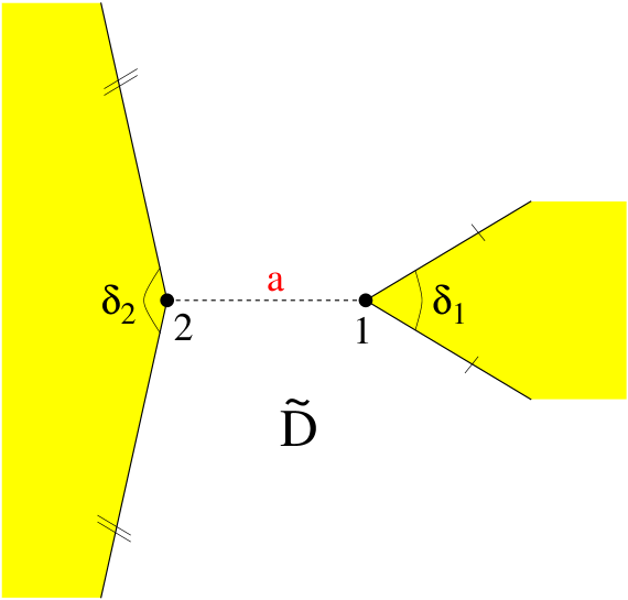
FIG. 1.: A constant ${\tilde{t}}$ surface of the fundamental domain for a static spacetime. The parts not belonging to the fundamental domain are shown as shaded. The particle world lines are orthogonal to the plane of the paper, and the orthogonal spatial distance of the world lines is $a$. The boundary segments marked by a single (double) stroke are identified by a rotation about particle $1$ ($2$) by the angle $\delta_{1}$ ($\delta_{2}$).

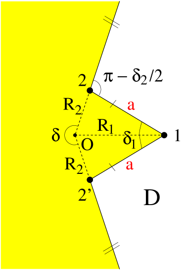
FIG. 2.: A constant $T$ surface of the fundamental domain $D$ for the static spacetime of figure 1. The corner labelled $1$ is at the first particle, and the corners labelled $2$ and $2^{\prime}$ are at the second particle. The particle world lines are orthogonal to the surface. The single-stroked boundaries are identified by a rotation about particle $1$ by the angle $\delta_{1}$, and the double-stroked boundaries are identified by a rotation about the (fictitious) origin $O$ by the angle $\delta=\delta_{1}+\delta_{2}$. Note that $O$ lies outside $D$. The (fictitious) distances $R_{i}$ of the particles from $O$ are given by (III B).

FIG. 3.: The boundary of the fundamental domain $D$ for the static spacetime in the Minkowski coordinates $(T,X,Y)$. $D$ is behind the boundary, and the parameters are $\delta_{1}=2\pi/5$, $\delta_{2}=4\pi/5$, and $a=1$. The viewpoint is on the negative $X$-axis. The grid on the two segments between the particles is adapted to the identification of these segments, and similarly for the grid on the two segments reaching the infinity. Note that the identifications do not affect the Minkowski time coordinate $T$.

FIG. 4.: A constant ${\tilde{t}}$ surface of the fundamental domain $\tilde{D}$ for a spacetime with colliding particles. The world line of particle $1$ is orthogonal to the plane of the paper, while the world line of particle $2$ has the boost parameter $\beta\neq 0$. For $\beta>0$ ($\beta<0$), particle $2$ is moving to the left (right), and the surface shown is at ${\tilde{t}}>0$ (${\tilde{t}}<0$). The spatial distance of the particles in the constant ${\tilde{t}}$ surface, along the dashed line, is ${\tilde{t}}\tanh\beta$. The angle ${\tilde{\delta}}_{2}$ is determined by $\delta_{2}$ and $\beta$ as the unique solution to $\cos({\tilde{\delta}}_{2}/2)=c_{2}\left(1+s_{2}^{2}\sinh^{2}\beta\right)^{-1/2}$ in the interval $0<{\tilde{\delta}}_{2}<2\pi$. The single-stroked (double-stroked) boundaries are identified by a rotation about the world line of particle $1$ ($2$) by the angle $\delta_{1}$ ($\delta_{2}$). Note that equation (8) implies $\delta_{1}+{\tilde{\delta}}_{2}<2\pi$, even when one of the defect angles is greater than $\pi$: this guarantees that the straight lines in the figure, at the boundaries of the $\tilde{D}$, always reach the infinity without intersecting.

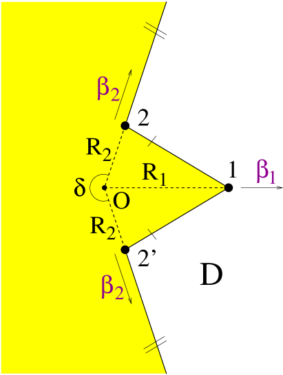
FIG. 5.: A constant $T$ surface of the fundamental domain $D$ for the spacetime with colliding particles. The corner labelled $1$ is at the first particle, and the corners labelled $2$ and $2^{\prime}$ are at the second particle. The world lines of the particles have the nonvanishing boost parameters $\beta_{i}$ (III C) with respect to the Minkowski coordinates $(T,X,Y)$. For $\beta>0$, $\beta_{i}$ and $T$ are positive and the velocities are in the directions shown; for $\beta<0$, $\beta_{i}$ and $T$ are negative, and the directions are the opposite. The single-stroked boundaries are identified by a rotation in the spacetime about the world line of particle $1$ by the angle $\delta_{1}$. The double-stroked boundaries are identified by (2). The distances of the particles from $O$ in (the extension beyond $D$ of) the constant $T$ surface are $R_{i}:=T\tanh\beta_{i}$.

FIG. 6.: The boundary of the fundamental domain $D$ for the colliding-particle spacetime in the Minkowski coordinates $(T,X,Y)$. The collision is in the past, $D$ is behind the boundary, and the parameters are $\delta_{1}=2\pi/5$, $\delta_{2}=4\pi/5$, and $\beta=0.2$. The viewpoint is at $(T,X,Y)=(0.7,-2,0)$. The grid is adapted to the identifications of the boundaries as in figure 3. Note that the identifications do not affect the Minkowski time coordinate $T$.

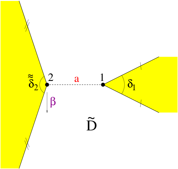
FIG. 7.: The surface ${\tilde{t}}=0$ of the fundamental domain $\tilde{D}$ for a spinning spacetime. The angle ${\tilde{\tilde{\delta}}}_{2}$ is determined by $\delta_{2}$ and $\beta$ as the unique solution to $\cos({\tilde{\tilde{\delta}}}_{2}/2)=c_{2}\left(1-s_{2}^{2}\tanh^{2}\beta\right)^{-1/2}$ in the interval $0<{\tilde{\tilde{\delta}}}_{2}<2\pi$. The extension of $\tilde{D}$ beyond the surface ${\tilde{t}}=0$ is described in the text. In the spacetime, single-stroked (double-stroked) boundary segments are identified by a rotation about the world line of particle $1$ ($2$) by the angle $\delta_{1}$ ($\delta_{2}$). The rotation about particle $1$ takes the ${\tilde{t}}=0$ sections of the single-stroked boundary segments to each other, but the rotation about particle $2$ does not take the ${\tilde{t}}=0$ sections of the double-stroked boundary segments to each other.

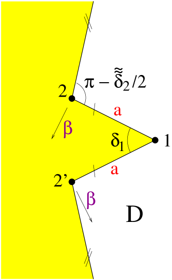
FIG. 8.: A surface of the fundamental domain $D$ for a spinning spacetime. We have first cut $\tilde{D}$ into two along a timelike surface that connects the world lines of the particles, as explained in the text. We have then rotated the two halves with respect to each other about the world line of particle $1$ so that the wedge originally at particle $1$, in figure 7 on the right, closes. The corner labelled $1$ is at the first particle, and the corners labelled $2$ and $2^{\prime}$ are at the second particle. In the spacetime, the single-stroked (double-stroked) boundary segments are identified as described in the text.

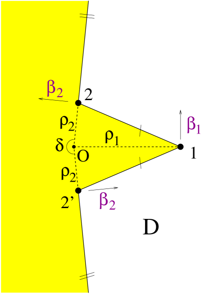
FIG. 9.: A spatial section of $D$ for a spinning spacetime at $\sigma=0$. The figure shows the projection to the $(X,Y)$-plane and suppresses the coordinate $T$: if the plane of the paper is at $T=0$, then the corner labelled $1$ is in this plane, while the corner labelled $2$ is above and the corner labelled $2^{\prime}$ is below this plane for $\beta>0$, and conversely for $\beta<0$. $\beta_{i}$, given by (III C), are the boost parameters of the particle trajectories with respect to the coordinates $(T,X,Y)$: for $\beta>0$, $\beta_{i}$ are positive and the velocities are in the directions shown, whereas for $\beta<0$, $\beta_{i}$ are negative and the directions are the opposite. $\rho_{1}$ and $\rho_{2}$ are as given in (III D). The single-stroked boundaries (neither of which is parallel to the plane of the paper) are identified by a rotation in the spacetime about the world line of particle $1$ by the angle $\delta_{1}$. The double-stroked boundaries (each of which is parallel to the plane of the paper but not in this plane) are identified by (2). Note that the origin of the $(X,Y)$ plane, labelled $O$, is outside $D$.

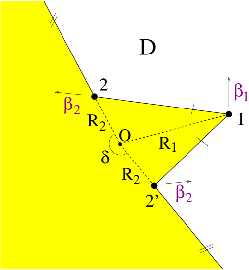
FIG. 10.: A spatial section of $D$ for a spinning spacetime at $\sigma>0$. The coordinate $T$ is suppressed as in figure 9. The single-stroked (double-stroked) boundaries are identified as in figure 9. $R_{1}$ and $R_{2}$ are given by (III D).

FIG. 11.: The boundary of the fundamental domain $D$ for the spinning spacetime in the Minkowski coordinates $(T,X,Y)$. $D$ is behind the boundary, and the parameters are $\delta_{1}=2\pi/5$, $\delta_{2}=4\pi/5$, $a=1$, and $\beta=0.2$. The viewpoint is on the negative $X$-axis. The grid is adapted to the respective identifications of the boundaries as in figures 3 and 6. Note how the identifications affect the Minkowski time coordinate $T$.

FIG. 12.: The fundamental half-strip $\Omega:=\left\{(\lambda,\omega)\mid\lambda>0,-\pi<\omega<\pi\right\}$ on the surface $\Sigma$. On the boundary of $\Omega$, particle $1$ is at the dashed line $\lambda=0$, while the points labelled $2$ and $2^{\prime}$, respectively at $(\lambda,\omega)=(1,\pm\pi)$, are both at the second particle. The boundary segments indicated by a single (respectively double) stroke are identified. The dashed lines $\lambda=\lambda_{i}$, $i\in\{0,1,2\}$, divide $\Omega$ into regions in which the gauge choice is as explained in the text.

- [1] Carlip S 1998 Quantum Gravity in 2+1 Dimensions (Cambridge University Press, Cambridge, England)
- [2] Deser S, Jackiw R and ’t Hooft G 1984 Ann. Phys. (N.Y.) 152 220
- [3] Deser S and Jackiw R 1984 Ann. Phys. (N.Y.) 153 405
- [4] ’t Hooft G 1988 Commun. Math. Phys. 117 685
- [5] Gott J R 1991 Phys. Rev. Lett. 66 1126
- [6] Ori A 1991 Phys. Rev. D 44 R2214
- [7] Deser S, Jackiw R and ’t Hooft G 1992 Phys. Rev. Lett. 68 267
- [8] Carroll S M, Farhi E, Guth A and Olum K D 1994 Phys. Rev. D 50 6190 [gr-qc/9404065]
- [9] Carroll S M, Farhi E and Guth A 1992 Phys. Rev. Lett. 68 263; Erratum, 3368
- [10] Cutler C 1992 Phys. Rev. D 45 487
- [11] ’t Hooft G 1992 Class. Quantum Grav. 9 1335
- [12] ’t Hooft G 1993a Class. Quantum Grav. 10 1023
- [13] Headrick M P and Gott J R 1994 Phys. Rev. D 50 7244
- [14] Carlip S 1989 Nucl. Phys. B 324 106
- [15] Cappelli A, Ciafaloni M and Valtancoli P 1991 Phys. Lett. 273B 431 [hep-th/9110020]
- [16] Cappelli A, Ciafaloni M and Valtancoli P 1992 Nucl. Phys. B 369 669
- [17] ’t Hooft G 1993b Class. Quantum Grav. 10 1653 [gr-qc/9305008]
- [18] Bellini A, Ciafaloni M and Valtancoli P 1995a Phys. Lett. 357B 532 [hep-th/9507076]
- [19] Bellini A, Ciafaloni M and Valtancoli P 1995b Nucl. Phys. B 454 449 [hep-th/9507077]
- [20] Bellini A, Ciafaloni M and Valtancoli P 1996 Nucl. Phys. B 462 453 [hep-th/9511207]
- [21] Welling M 1997 Class. Quantum Grav. 14 3313 [gr-qc/9703058]
- [22] Welling M 1998 Class. Quantum Grav. 15 613 [gr-qc/9704067]
- [23] Matschull H-J and Welling M 1998 Class. Quantum Grav. 15 2981 [gr-qc/9708054]
- [24] Menotti P and Seminara D 1999 “ADM approach to 2+1 dimensional gravity coupled to particles” Preprint IFUP-TH 39/99, LPTENS-99/24, hep-th/9907111.
- [25] Misner C W, Thorne K S, and Wheeler J A 1973 Gravitation (Freeman, San Francisco) Chapter 19
- [26] Regge T and Teitelboim C 1974 Ann. Phys. (N.Y.) 88 286
- [27] Beig R and ó Murchadha N 1987 Ann. Phys. (N.Y.) 174 463
- [28] Henneaux M 1984 Phys. Rev. D 29 2766
- [29] Ashtekar A and Varadarajan M 1994 Phys. Rev. D 50 4944 [gr-qc/9406040]
- [30] Achúcarro A and Townsend P K 1986 Phys. Lett. 180B 85
- [31] Witten E 1988 Nucl. Phys. B 311 46
- [32] Ashtekar A 1991 Lectures on Non-Perturbative Canonical Gravity (World Scientific, Singapore) Chapter 17
- [33] Romano J D 1993 Gen. Rel. Grav. 25 759 [gr-qc/9303032]
- [34] Louko J and Marolf D M 1994 Class. Quantum Grav. 11 311 [gr-qc/9308018]
- [35] Gibbons G W, Ruiz Ruiz F and Vachaspati T 1990 Commun. Math. Phys. 127 295
- [36] Louko J and Matschull H-J in preparation
- [37] Deser S and Steif A R 1992 Class. Quantum Grav. 9 L153 [hep-th/9208018]
- [38] Deser S, McCarthy J and Steif A R 1994 Nucl. Phys. B 412 305 [hep-th/9307092]
- [39] Steif A R 1996 Phys. Rev. D 53 5527 [gr-qc/9511053]
- [40] Matschull H-J 1999 Class. Quantum Grav. 16 1069 [gr-qc/9809087]
- [41] Holst S and Matschull H-J 1999 Class. Quantum Grav. 16 3095 [gr-qc/9905030]
- [42] Horowitz G T and Itzhaki N 1999 JHEP 9902 010 [hep-th/9901012]
- [43] Danielsson U H, Keski-Vakkuri E and Kruczenski M 1999 Nucl. Phys. B 563 279 [hep-th/9905227]
- [44] Balasubramanian V and Ross S F 2000 Phys. Rev. D 61 044007 [hep-th/9906226]
- [45] Ohta T and Mann R B 1996 Class. Quantum Grav. 13 2585 [gr-qc/9605004]; Mann R B and Ohta T 1997a Phys. Rev. D 57 4723 [gr-qc/9611008]; Mann R B and Ohta T 1997b Class. Quantum Grav. 14 1259 [gr-qc/9607016]; Mann R B, Robbins D and Ohta T 1999a Phys. Rev. Lett. 82 3738 [gr-qc/9811061]; Mann R B, Robbins D and Ohta T 1999b Phys. Rev. D 60 104048 [gr-qc/9906066]