[

Wave Function of a Brane-like Universe

Abstract

Within the mini-superspace model, brane-like cosmology means performing the variation with respect to the embedding (Minkowski) time $\tau$ before fixing the cosmic (Einstein) time $t$. The departure from Einstein limit is parameterized by the ’energy’ conjugate to $\tau$, and characterized by a classically disconnected Embryonic epoch. In contrast with canonical quantum gravity, the wave-function of the Universe is (i) $\tau$-dependent, and (ii) vanishes at the Big Bang. Hartle-Hawking and Linde proposals dictate discrete ’energy’ levels, whereas Vilenkin proposal resembles $\alpha$-disintegration.

]

In this paper, the Universe is viewed as a curved four-dimensional bubble[1] floating in a higher dimensional flat background. To discuss the quantum disintegration of such a Brane-like Universe and derive the corresponding time-dependent and Big-Bang resistant wave function, we restrict ourselves to the framework of the mini-superspace model[2].

Assuming the Universe to be homogeneous, isotropic, and closed, the Friedman-Robertson-Walker (FRW) line element can be written in the form

$$ds^{2}=\sigma^{2}\left[-({\dot{\tau}}^{2}-{\dot{a}}^{2})dt^{2}+a^{2}(t)d\Omega_{3}^{2}\right]~{},$$ (1)

where $d\Omega_{3}^{2}$ denotes the metric of a unit $3$-sphere, and $\sigma^{2}\equiv\frac{4G}{3\pi}$ is a normalization factor. One may still exercise of course the gauge freedom of fixing $\tau(t)$. However, the more general form helps us keep track of the way the FRW manifold is embedded within a $5$-dim Minkowski spacetime

$$ds^{2}_{5}=\sigma^{2}\left[-d\tau^{2}+da^{2}+a^{2}d\Omega_{3}^{2}\right]~{}.$$ (2)

A pedagogical case of sufficient complexity involves a positive cosmological constant $\Lambda$. The corresponding mini-Lagrangian, defined by $I=\int{\cal L}dt$, is given by

$${\cal L}=-\left(\frac{a{\dot{a}}^{2}}{\sqrt{{\dot{\tau}}^{2}-{\dot{a}}^{2}}}+a(H^{2}a^{2}-1)\sqrt{{\dot{\tau}}^{2}-{\dot{a}}^{2}}\right)~{},$$ (3)

where $H^{2}\equiv\frac{16\pi G}{3}\Lambda$.

$\bullet$ The standard mini-superspace prescription is to impose the so-called cosmic gauge, namely ${\dot{\tau}}^{2}-{\dot{a}}^{2}=1$, and treat $a(t)$ as a single canonical variable. This way, the variation with respect to $a(t)$ gives rise to Raychaudhuri equation, and the complementary evolution equation

$${\dot{a}}^{2}+1=H^{2}a^{2}$$ (4)

is then nothing but the Arnowitt-Deser-Misner (ADM) Hamiltonian constraint ${\cal H}=0$. Let $P=-2a{\dot{a}}$ be the momentum conjugate to $a$, the Hamiltonian takes the form

$${\cal H}=-\frac{1}{4a}\left(P^{2}+V(a)\right)~{},$$ (5)

involving the familiar potential

$$V(a)=4a^{2}\left(1-H^{2}a^{2}\right)~{}.$$ (6)

Quantization means replacing $\displaystyle{P\rightarrow-i\frac{\delta}{\delta a}}$ and imposing the Wheeler-DeWitt (WDW) equation ${\cal H}\Psi(a)=0$ on the wave function of the Universe.

$\bullet$ The non-standard procedure would be to allow both $a(t)$ and $\tau(t)$ to serve as two independent canonical variables. The variation with respect to $\tau(t)$ results in a simple conservation law. Owing to ${\cal L}(a,\dot{a},\dot{\tau})$, the ’energy’ $\omega$ conjugate to $\tau$ is conserved. Imposing the cosmic gauge ${\dot{\tau}}^{2}-{\dot{a}}^{2}=1$ only at this stage, we can rearrange the ’energy’ conservation equation into a generalized evolution equation

$${\dot{a}}^{2}+1=\xi H^{2}a^{2}~{},$$ (7)

with $\xi(a)$ being a root of

$$\xi(\xi-1)^{2}=\frac{\omega^{2}}{H^{6}a^{8}}~{}.$$ (8)

Eq.(7) is recognized as the Regge-Teitelboim (RT)[3, 4] equation of motion, with Einstein limit approached as $\omega\rightarrow 0$, that is $\xi\rightarrow 1$ (the physical brunch is identified with $\xi\geq 1$). This comes with no surprise, given that RT canonical variables are in fact the embedding coordinates. Recalling that classical RT-cosmology[4] involves only one independent equation of motion, the equation arising by varying with respect to $a(t)$ is superfluous.

The $2$-momentum $\displaystyle{P_{\alpha}=(\frac{\delta{\cal L}}{\delta{\dot{\tau}}},\frac{\delta{\cal L}}{\delta{\dot{a}}})}$ is given by

$$P_{\tau} = \left[\left(\frac{\dot{a}}{\sqrt{{\dot{\tau}}^{2}-{\dot{a}}^{2}}}\right)^{2}+1-H^{2}a^{2}\right]\frac{a\dot{\tau}}{\sqrt{{\dot{\tau}}^{2}-{\dot{a}}^{2}}}~{},$$ (10)

$$P_{a} = -\left[\left(\frac{\dot{a}}{\sqrt{{\dot{\tau}}^{2}-{\dot{a}}^{2}}}\right)^{2}+3-H^{2}a^{2}\right]\frac{a\dot{a}}{\sqrt{{\dot{\tau}}^{2}-{\dot{a}}^{2}}}~{}.$$ (11)

The $t$-derivatives which enter eq.(Wave Function of a Brane-like Universe) conveniently furnish a time-like unit $2$-vector

$$n^{\alpha}\equiv\left(\frac{\dot{\tau}}{\sqrt{{\dot{\tau}}^{2}-{\dot{a}}^{2}}},\frac{\dot{a}}{\sqrt{{\dot{\tau}}^{2}-{\dot{a}}^{2}}}\right)~{},~{}~{}n^{2}+1=0~{}.$$ (12)

Invoking now a $(\dot{\tau},\dot{a})$-independent matrix

$$\rho^{\alpha}_{\,\beta}=\left(\begin{array}[]{cc}2a(H^{2}a^{2}-1)&0\\ 0&2a(H^{2}a^{2}-2)\end{array}\right)~{},$$ (13)

$P^{\alpha}$ can be put in the compact form

$$P^{\alpha}=\frac{1}{2}(n\rho n)n^{\alpha}+\rho^{\alpha}_{\beta}n^{\beta}~{},$$ (14)

after subtracting $a(H^{2}a^{2}-1)(n^{2}+1)n^{\alpha}$. A naive attempt to solve $n^{\alpha}(\rho,P)$, as apparently dictated by the Hamiltonian formalism, and substitute into the constraint $n^{2}+1=0$, falls short. The cubic equation involved does not admit a simple solution, and the resulting constraint is anything but quadratic in the momenta.

The way out, that is linearizing the problem, involves the definition of an independent quantity $\lambda$, such that

$$n\rho n+2\lambda=0~{}.$$ (15)

Off the Einstein limit, $\lambda$ is not an eigenvalue of $\rho^{\alpha}_{\,\beta}$, and we can solve for $n^{\alpha}(\rho,P,\lambda)$ to find

$$n^{\alpha}=\left[\left(\rho-\lambda I\right)^{-1}\right]^{\alpha}_{\,\beta}P^{\beta}~{}.$$ (16)

This allows us to finally convert the combined constraints $n^{2}+1=0$ and $n\rho n+2\lambda-\lambda(n^{2}+1)=0$ into

$$\left\{\begin{array}[]{c}P(\rho-\lambda I)^{-2}P+1=0~{},\\ P(\rho-\lambda I)^{-1}P+\lambda=0~{}.\end{array}\right.$$ (17)

The first equation is the derivative with respect to $\lambda$ of the other. This suggests that $\lambda$ be elevated to the level of a canonical non-dynamical variable in the forthcoming Hamiltonian formalism.

Needless to say, the above seems to be a tip of a bigger iceberg, a mini-superspace version of Brane-like gravity. Indeed, carrying out the (say) $10$-dim RT embedding of the $4$-dim ADM formalism, we have recently derived the quadratic Hamiltonian[5]

$${\cal H}=\frac{1}{2}N\left[P_{A}\left((\rho-\lambda I)^{-1}\right)^{AB}P_{B}+\lambda\right]+N^{i}y^{A}_{\,,i}P_{A}~{},$$ (18)

where the novel Lagrange multiplier $\lambda$ accompanies the standard non-dynamical variables, the lapse function $N$ and the shift vector $N^{i}$. To shed light on the matrix $\rho^{AB}$, one infers that

$$\frac{\rho^{AB}}{2\sqrt{h}}=(h^{ia}h^{jb}-h^{ij}h^{ab})y^{A}_{\,|ab}y^{B}_{\,|ij}+\left({\cal R}^{(3)}+6H^{2}\right)\eta^{AB}~{},$$ (19)

with ${\cal R}^{(3)}$ denoting the $3$-dim Ricci scalar constructed by means of the spatial $3$-metric $h_{ij}=\eta_{AB}y^{A}_{|i}y^{B}_{|j}$.

The quantum theory dictates ${\displaystyle P_{A}\rightarrow-i\frac{\delta}{\delta y^{A}}}$. The corresponding wave function $\Psi(\tau,a)$ is subject to two Virasoro-type constraints. The so-called momentum constraint equation $\displaystyle{y^{A}_{,i}\frac{\delta\Psi}{\delta y^{A}}=0}$, which is trivially satisfied at the mini-superspace level, is accompanied by a bifurcated WDW equation

$$\left\{\begin{array}[]{c}\displaystyle{\frac{\delta}{\delta y^{A}}\left((\rho-\lambda I)^{-1}\right)^{AB}\frac{\delta}{\delta y^{B}}\Psi=\lambda\Psi}~{},\\ \displaystyle{\frac{\delta}{\delta y^{A}}\left((\rho-\lambda I)^{-2}\right)^{AB}\frac{\delta}{\delta y^{B}}\Psi=\Psi}~{}.\end{array}\right.$$ (20)

Given the diagonal $\rho^{\alpha}_{\,\beta}$ specified by eq.(13), and up to all sorts of order ambiguities, the mini-superspace wave function $\Psi(\tau,a)$ obeys

$$-\frac{\partial^{2}\Psi}{\partial\tau^{2}} = \xi(\xi-1)^{2}H^{6}a^{8}\Psi~{},$$ (22)

$$-\frac{\partial^{2}\Psi}{\partial a^{2}} = a^{2}\left[2+(\xi-1)H^{2}a^{2}\right]^{2}(-1+\xi H^{2}a^{2})\Psi~{},$$ (23)

where the $\lambda\leftrightarrow\xi$ dictionary reads

$$\lambda\equiv a\left[(\xi+1)H^{2}a^{2}-2\right]~{}.$$ (24)

The separation of variables is accomplished by substituting $\Psi(\tau,a)=\psi(a)\chi(\tau)$. Eq.(23) then tells us that $\xi=\xi(a)$. In turn, eq.(22) can admit a solution only provided $\xi(a)$ is such that $\xi(\xi-1)^{2}H^{6}a^{8}=\omega^{2}$ is a constant. This is how the conserved ’energy’ $\omega$, introduced by eq.(8), enters the quantum game.

Altogether, the $\tau$-dependent wave function of the Universe acquires the familiar form

$$\Psi(\tau,a)=\psi(a)e^{-i\omega\tau}~{},$$ (25)

with the $\tau$-dependence dropping out at the Einstein limit. The radial component $\psi(a)$ satisfies the residual WDW equation

$$\left(-\frac{\partial^{2}}{\partial a^{2}}+V(a)\right)\psi=0~{},$$ (26)

where the modified potential, depicted in fig.(1), is given explicitly by

$$V(a)=a^{2}\left[2+(\xi-1)H^{2}a^{2}\right]^{2}(1-\xi H^{2}a^{2})~{}.$$ (27)

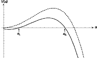
FIG. 1.: Wheeler-DeWitt potential for a Brane-like Universe (solid curve), and for Einstein Universe (dashed curve).

$V(a)$ admits a barrier provided $\omega H\leq\frac{2}{3\sqrt{3}}$, which we now adopt as the case of interest. The barrier is stretched between $a_{L}<a<a_{R}$, where $a_{L,R}$ are the two positive roots of $H^{2}a^{3}-a+\omega=0$. For $\omega H\ll 1$, the classical turning points are located at

$$a_{L}\simeq\omega~{},~{}~{}a_{R}\simeq H^{-1}(1-\frac{1}{2}\omega H)~{}.$$ (28)

At long distances, only a slight deviation from the original potential is detected, namely

$$V(a\gg\omega)\simeq 4a^{2}(1-H\omega-H^{2}a^{2})~{}.$$ (29)

But at short distances, a serendipitous well (with a surplus of ‘kinetic energy’ at the origin) makes its appearance

$$V(a\leq\omega)\simeq-\omega^{2}-3\omega^{4/3}a^{2/3}+4a^{2}~{}.$$ (30)

The emerging classically disconnected Embryonic epoch is the essence of brane-like quantum cosmology.

A theory of boundary conditions is still to be constructed. The situation is even more complicated in a scheme where the Big-Bang is classically alive and cannot be traded for a Euclidean conic-singularity-free pole. The Riemann tensor gets pathological as $a\rightarrow 0$, leaving us with no alternative but to interpret ’nothing’ [6] as

$$\Psi(\tau,a=0)=0~{}.$$ (31)

This way, following DeWitt[7] argument, we ’neutralize’ the Big Bang singularity by making the origin quantum mechanically inaccessible to wave packets.

At this stage, while sticking to the full Lorentzian picture, namely $\Psi=\psi(a)e^{-i\omega\tau}$ even under the potential barrier, our discussion bifurcates with respect to the left over boundary condition:

$\bullet$ Following Hartle-Hawking (HH)[8] or Linde (L)[9] proposals, where Hermiticity (real $\omega$) is the name of the game, the naive WKB wave function under the barrier is given by

$$\psi_{HH,L}(a_{L}<a<a_{R})\simeq\mp\frac{1}{\sqrt{V}}\exp\left[\pm\int_{a_{L}}^{a}\sqrt{V}da^{\prime}\right]~{},$$ (32)

respectively. The corresponding nucleation probability is

$${\cal P}\sim e^{{\displaystyle\pm 2\int_{a_{L}}^{a_{R}}\sqrt{V}da^{\prime}}}\simeq e^{{\displaystyle\pm\frac{4}{3H^{2}}(1-\frac{3}{2}H\omega)}}~{}.$$ (33)

The matching at $a=a_{R}$ yields a symmetric (antisymmetric) combination of equal strength outgoing and ingoing waves. The $a=a_{L}$ matching into the Embryonic zone would contradict the Big-Bang boundary condition eq.(31) unless

$$\exp\left[2i\left(\int_{0}^{a_{L}}\sqrt{-V}da^{\prime}-\frac{\pi}{4}\right)\right]=\pm 1~{}.$$ (34)

The result is ’energy’ (not to be confused with the energy $E=0$) quantization. To be specific, for $\omega H\ll 1$, we invoke eq.(30) and after some algebra derive the discrete ’energy’ spectrums

$$\omega^{HH,L}_{n}\simeq\sqrt{\frac{2}{3}(4n\pm 1)}~{},$$ (35)

such that $\omega^{L}_{min}=\sqrt{3}\omega^{HH}_{min}$.

Having a non-zero ground state ’energy’ $\omega_{min}$ is remarkable. It is the closest one can get to Einstein limit $\omega=0$. But what exactly do we mean by a ground state, and why does the Einstein limit make sense? A successful (presumably Euclidean) theory of boundary conditions must explain why is low $\omega$ preferable to high $\omega$.

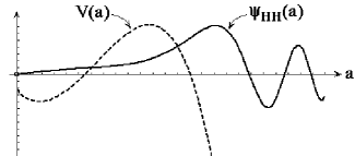
FIG. 2.: Hartle-Hawking ground state ($n=0$) wave function of a brane-like Universe (notice its vanishing at the Big Bang). The dashed curve being the underlying brane-like Wheeler-DeWitt potential.

$\bullet$ Vilenkin (V)[10] proposal on the other hand is characterized by an outgoing wave function

$$\psi_{V}(a>a_{R})\sim\frac{1}{\sqrt{-V}}\exp\left[i\int_{a_{R}}^{a}\sqrt{-V}da^{\prime}\right]~{}.$$ (36)

The WKB behavior of the wave function can then be traced back all the way to the origin where it is supposed to vanish. The consistency condition then reads

$$\exp\left[2i\left(\int_{0}^{a_{L}}\sqrt{-V}da^{\prime}-\frac{\pi}{4}\right)\right]\simeq\frac{1+4\theta^{2}}{1-4\theta^{2}}~{},$$ (37)

where $\theta\equiv e^{\int_{a_{L}}^{a_{R}}\sqrt{V}da^{\prime}}$ is the opacity coefficient. The latter equation can only be satisfied by a complex ’energy’ $\omega=\tilde{\omega}-\frac{1}{2}i\Gamma$. It should be noticed how the Hartle-Hawking (Linde) discrete spectrum, that is $\tilde{\omega}\rightarrow\omega_{n}^{HH(L)}$ followed by $\Gamma\rightarrow 0$, is recovered for $\theta\ll 1$ ($\theta\gg 1$). Altogether, the disintegration of Vilenkin bubble highly resembles $\alpha$-decay.

Euclidization is next. In the first glance it may look like the Lorentzian and the Euclidean regimes share the one and the same Embedding spacetime, and that Euclidization can be formulated in the language of the mini-superspace light-cone. However, a simple investigation reveals that a closed Euclidean FRW metric cannot be embedded within a flat Minkowski spacetime. It calls for a flat Euclidean background, attainable by means of Wick rotation $\tau\rightarrow\pm i\tau_{E}$ (with the corresponding cosmic gauge being $\dot{\tau_{E}}^{2}+\dot{a_{E}}^{2}=1$).

We are not in a position to tell whether Euclidean gravity is only a technical tool, serving to explain certain quantum and/or thermodynamic aspects of the Lorentzian theory, or perhaps has life of its own. This way or the other, the emerging picture is of a Euclidean manifold sandwiched between two Lorentzian regimes.

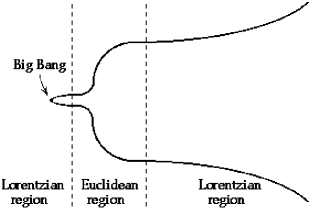
FIG. 3.: The Euclidean regime sandwiched between the Embryonic and the Expanding Lorentzian epochs.

The Euclidean time difference $\delta$ to travel back and forth the $a_{L}<a<a_{R}$ well of the upside down potential $-V$ is given by

$$\delta=2\int_{a_{L}}^{a_{R}}\frac{da}{\sqrt{1-\xi H^{2}a^{2}}}~{},$$ (38)

and takes the value

$$\delta\simeq\left\{\begin{array}[]{ccc}\frac{\pi}{H}\left(1-\frac{2}{\pi}\sqrt{\omega H}\right)&~{}~{}~{}\text{if}{}&\omega H\ll 1~{},\\ 4\sqrt{3}\omega&~{}~{}~{}\text{if}{}&\omega H=\frac{2}{3\sqrt{3}}~{}.\end{array}\right.$$ (39)

Recall two relevant facts: (i) The Euclidean manifold can be periodic in $t_{E}$. The allowed periodicities are restricted, however, to the sequence $\Delta t_{E}=N\delta$ ($N$ integer). (ii) At the Euclidean de-Sitter limit, where $\omega\rightarrow 0$, the Euclidean manifold must be periodic in $t_{E}$ with period $\Delta t_{E}=2\pi H^{-1}$, as otherwise a conic singularity is present. Combining these two facts, one can identify $t_{E}$ with $t_{E}+\Delta t_{E}$ provided

$$\Delta t_{E}=2\delta~{}.$$ (40)

In turn, our bubble Universe is characterized by a temperature $\displaystyle{T=\frac{1}{\Delta t_{E}}}$ and an entropy $\displaystyle{S=\frac{1}{4\pi}\Delta t_{E}^{2}}$.

The model discussed here has no pretension to be realistic. Its objective is primarily pedagogical, to concretely demonstrate (i) How to overcome the problem (absence) of time in canonical quantum gravity, and (ii) How to ’neutralize’, quantum-mechanically, the Big-Bang problem at the Lorentzian level. All this without upsetting the leading wave-function proposals. It remains to be understood though how to convert the emerging closed Universe into an open one (following perhaps Hawking-Turok[11] prescription), how does inflation enter the game (presumably along Linde[12] or Vilenkin[13] trails), and whether there exists some leftover experimental crumb. At any rate, several model independent features, notably the classically disconnected Embryonic epoch, are to be regarded as the finger-prints of the underlying theory. Brane-like Universe gravity constitutes a controlled deviation (automatic energy/momentum conservation) from Einstein gravity, with the latter regarded as the classical ground-state limit.

- [1] G.W. Gibbons and D.L. Wiltshire, Nucl. Phys. B287, 717 (1987); S. Coleman and F. DeLuccia, Phys. Rev. D21, 3305 (1980); R. Basu, A.H. Guth and A. Vilenkin, Phys. Rev. D44, 340 (1991).
- [2] B.S. DeWitt, Phys. Rev. 160, 1113 (1967); J.A. Wheeler, in Battelle Rencontres, p.242 (Benjamin NY, 1968); W.E. Blyth and C. Isham, Phys. Rev. D11, 768 (1975).
- [3] T. Regge and C. Teitelboim, in Proc. Marcel Grossman, p.77 (Trieste, 1975); S. Deser, F.A.E. Pirani, and D.C. Robinson, Phys. Rev. D14, 3301 (1976).
- [4] A. Davidson, (gr-qc/9710005).
- [5] A. Davidson and D. Karasik, (honorable mentioned, Grav. Res. Found. 1998).
- [6] E.P. Tyron, Nature 246, 396 (1973).
- [7] J.D. Barrow and R. Matzner, Phys. Rev. D21, 336 (1980); M.J. Gotay and J. Demaret, Phys. Rev. D28, 2402 (1983).
- [8] S.W. Hawking and I.G. Moss, Phys. Lett. 110B, 35 (1982); J. Hartle and S.W. Hawking, Phys. Rev. D28, 2960 (1983); J.J. Halliwell and S.W. Hawking, Phys. Rev. D31, 1777 (1985).
- [9] A.D. Linde, Nuovo Cimento 39, 401 (1984); A.D. Linde, Sov. Phys. JETP 60, 211 (1984);
- [10] A. Vilenkin, Phys. Lett. 117B, 25 (1982); A. Vilenkin, Phys. Rev. D30, 509 (1984); A. Vilenkin, Phys. Rev. D50, 2581 (1994).
- [11] N. Turok and S.W. Hawking (hep-th/9802030,9803156);
- [12] A.D. Linde (gr-qc/980238).
- [13] A. Vilenkin (hep-th/9803084).