Cosmic Solenoids:
Minimal Cross-Section and Generalized Flux Quantization

Abstract

A self-consistent general relativistic configuration describing a finite cross-section magnetic flux tube is constructed. The cosmic solenoid is modeled by an elastic superconductive surface which separates the Melvin core from the surrounding flat conic structure. We show that a given amount $\Phi$ of magnetic flux cannot be confined within a cosmic solenoid of circumferential radius smaller than ${\displaystyle\frac{\sqrt{3G}}{2\pi c^{2}}\Phi}$ without creating a conic singularity (the expression for the angular deficit is different from that naively expected). Gauss-Codazzi matching conditions are derived by means of a self-consistent action. The source term, representing the surface currents, is sandwiched between internal and external gravitational surface terms. Surface superconductivity is realized by means of a Higgs scalar minimally coupled to projective electromagnetism. Trading the ’magnetic’ London phase for a dual ’electric’ surface vector potential, the generalized quantization condition reads: ${\displaystyle\frac{e}{hc}\Phi+\frac{1}{e}Q=n}$ with $Q$ denoting some dual ’electric’ charge, thereby allowing for a non-trivial Aharonov-Bohm effect. Our conclusions persist for dilaton gravity provided the dilaton coupling is sub-critical.

]

I Introduction

The Dirac procedure of squeezing a magnetic flux tube, while keeping its total magnetic flux $\Phi$ fixed, plays an important role in theoretical physics. It is usually assumed that one can shrink the solenoid into a thin magnetic flux string characterized by the potential

$$A_{\mu}dx^{\mu}=Nd\phi=\frac{N}{r^{2}}(xdy-ydx)~{}.$$ (1)

Such a measure zero infinitely-long flux string is of course classically invisible, but can still allow for a non-trivial quantum mechanical Aharonov-Bohm effect[1]. Furthermore, if the total magnetic flux is properly quantized, namely

$$\frac{e\Phi}{hc}=n~{},$$ (2)

the flux string can be regarded an artifact since it cannot be detected by test particles carrying quantized electric charge in units of $e$. In which case, eq.(1) is nothing but a pure gauge. By the same token, the semi-infinite magnetic flux string attached to a Dirac magnetic monopole[2], carrying magnetic charge $g$, becomes physically irrelevant in case that

$$\frac{eg}{hc}=\frac{1}{2}n~{}.$$ (3)

On dimensional grounds, however, it is clear that a string is not really capable of fully representing the case of an arbitrarily narrow tube. In particular, the innocent looking magnetic flux string configuration eq.(1) is apparently sourceless. To keep track of the source, one should consider a magnetic flux tube of finite radius, and let a surface current constitute the source. This way, to keep the total magnetic flux finite, the surface current gets infinitely large as the tube becomes infinitesimally narrow.

The situation is conceptually and drastically changed once gravity (or string theory) enters the game. In this paper, a self-consistent general relativistic configuration describing a finite cross-section cosmic solenoid is constructed. The cosmic solenoid is modeled by an elastic superconductive surface which separates the curved inner core from the surrounding flat conic structure. Any attempt to squeeze the cosmic solenoid, while holding its total magnetic flux $\Phi$ fixed, comes with a cosmic penalty. In the extreme, if trying to imprison any given amount of magnetic flux within a tube of a sub-critical cross-section, one pays the ultimate price of closing the surrounding space and creating a conic singularity.

Adopting the $\hbar=c=1$ units, here are some exact spacetime configurations[3] relevant to our discussion:

$\bullet$ The general stationary cylindrically symmetric vacuum solution of Einstein equations is given by

$$ds^{2}=-\Omega(dt+Vd\phi)^{2}+\omega(dr^{2}+dz^{2})+\frac{r^{2}}{\Omega}d\phi^{2}~{},$$ (4)

where we have used the notations

$$\begin{array}[]{rcl}\omega(r)&=&\displaystyle{r^{\frac{1}{2}(n^{2}-1)}}~{},\vspace{6pt}\\ \Omega(r)&=&\displaystyle{r\left(\frac{\alpha}{r^{n}}-\beta r^{n}\right)}~{},\vspace{6pt}\\ V(r)&=&\displaystyle{\sqrt{\frac{\beta}{\alpha}}\frac{r^{n+1}}{\Omega}}~{}.\end{array}$$ (5)

$\bullet$ The static solution calls for $V(r)=const$, and can be put in the familiar $(a,b,c)$ Kasner form

$$ds^{2}=-r^{2a}dt^{2}+r^{2b}dz^{2}+dr^{2}+\gamma^{2}r^{2c}d\phi^{2}~{},$$ (6)

with the various parameters subject to

$$\begin{array}[]{c}a+b+c=1~{},\vspace{6pt}\\ a^{2}+b^{2}+c^{2}=1~{}.\end{array}$$ (7)

The factor $\gamma$ acquires a (global) physical meaning once the periodicity notation is specified, say

$$\Delta\phi=2\pi~{}.$$ (8)

The only asymptotically-flat Kasner solution is the locally-flat yet globally conic $(0,0,1)$ solution. The conic defect, reflecting the topological charge of the sectional $2$-metric, measures the variation of the invariant circumferential radius $\rho(r)$ with respect to the invariant radial distance $R(r)$. Given the flat Kasner metric eq.(6), for which $\rho=\gamma r$ and $R=r$, one finds

$$\frac{d\rho}{dR}=\gamma~{},$$ (9)

corresponding to a deficit angle of $2\pi(1-\gamma)$. As long as $\gamma\geq 0$, the outer space is open, but $\gamma<0$ takes us to the back side of the cone. In which case, the outer space is closed and exhibits a singular point at a finite distance.

A well known example is the space surrounding a cosmic string [4, 5, 6]. The corresponding Vilenkin conic defect[4] reads

$$\gamma=1-4\mu G~{},$$ (10)

where $\mu$ is the energy density per unit length of the string. The physical demand $\gamma\geq 0$ then leads to the consistency condition $\displaystyle{\mu\leq\frac{1}{4G}}$.

$\bullet$ The general cylindrically-symmetric static solution of Einstein-Maxwell equations involving a longitudinal magnetic field (caused by an angular current) is referred to as the Witten solution[7]

$$ds^{2}=\omega^{4}W^{2}(-dt^{2}+dr^{2})+W^{2}dz^{2}+\frac{r^{2}}{W^{2}}d\phi^{2}~{},$$ (11)

where the Witten factor $W(r)$ is given by

$$W(r)=\frac{\alpha}{r^{n-1}}+\beta r^{n+1}~{}.$$ (12)

This metric can be viewed as a soliton connecting two Kasner regimes, namely $\left(\frac{n(n-1)}{n^{2}-n+1},\frac{1-n}{n^{2}-n+1},\frac{n}{n^{2}-n+1}\right)$ and its $n\rightarrow-n$ companion.

$\bullet$ Regularity at the $r=0$ axis of symmetry (at the expense of a generic singularity at $r\rightarrow\infty$) singles out the Lorentz invariant (along the $z$-axis) $\alpha^{2}=n=1$ case, known as the Melvin solution[8]

$$ds^{2}=M^{2}(r)(-dt^{2}+dz^{2}+dr^{2})+\frac{r^{2}}{M^{2}(r)}d\phi^{2}~{},$$ (13)

where the Melvin factor $M(r)$ is given by

$$M(r)\equiv 1+\frac{1}{4}GB^{2}r^{2}~{}.$$ (14)

It is accompanied by the electromagnetic configuration

$$\begin{array}[]{rcl}A_{\phi}&=&\displaystyle{\frac{Br^{2}}{2M(r)}}~{},\vspace{6pt}\\ F_{r\phi}&=&\displaystyle{\frac{Br}{M^{2}(r)}}~{}.\end{array}$$ (15)

One observes that the magnetic flux is practically confined within a tube of radius $\displaystyle{\frac{2}{\sqrt{G}}B}$, where $B$ is the value of the magnetic field at the origin (in our form notations, $\displaystyle{B_{z}=\frac{1}{r}F_{r\phi}}$). As expected, the Melvin solution represents a soliton which connects the only two Kasner branches which are allowed by partial Lorentz invariance, namely

$$(0,0,1)\longleftrightarrow(\frac{2}{3},\frac{2}{3},-\frac{1}{3})~{}.$$ (16)

Whereas the $(0,0,1)$ branch, associated with $r\rightarrow 0$, is regular, the $(\frac{2}{3},\frac{2}{3},-\frac{1}{3})$ branch, associated with $r\rightarrow\infty$, is not only singular but furthermore exhibits a vanishing circumferential radius.

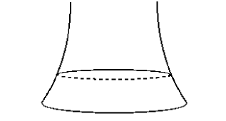
FIG. 1.: Melvin bone: The 2-dim surface (as embedded in flat 3-space) characterized by the sectional 2-metric $ds^{2}=M^{2}(r)dr^{2}+r^{2}M^{-2}(r)d\phi^{2}$.

In light of this, a cosmic solenoid should be constructed by pasting together two manifolds. The core of the tube, which contains the magnetic flux and consequently exhibits the Melvin geometry, is wrapped by a flat Kasner Universe which carries no magnetic fields but has a generic conic structure. These manifolds are separated by an elastic superconductive surface hosting the surface currents. In a self-consistent model like ours, these surface currents are expected to be dynamically created by some surface fields minimally coupled to projective electromagnetism. The corresponding self-consistent action principle must not only govern the equations of motion, but also the matching conditions (including in particular the Gauss-Codazzi formalism) of the various fields involved. The latter include the gravitational field $g_{\mu\nu}$, the electromagnetic vector potential $A_{\mu}$, the optional dilaton field $\eta$, and a variety of $(2+1)$-dimensional surface fields. It is only after such a model is analytically constructed, that one is able to analyze the case from the shrinking circumferential radius point of view.

This paper is organized as follows. First, we present the tenable action principle and derive the corresponding equations of motion and the attached matching conditions. In this Lagrangian formalism, the surface source term is sandwiched between the internal and the external gravitational surface terms. This is the prescription behind the field theoretical recovery of the Gauss-Codazzi and the electromagnetic matching equations. We are after the cylindrically symmetric static solution, focusing our attention on two parameters, namely the circumferential radius of the tube and the conic defect of the surrounding space-time. Surface superconductivity is realized by means of a Higgs scalar minimally coupled to projective electromagnetism, thereby establishing the linkage between the circumferential radius and the conic defect. The main result of this linkage is that the circumferential radius $\rho$ cannot be arbitrarily small unless the surrounding space-time suffers a singularity. To be more specific (and use momentarily the full units),

ρmin≥3G2πc2Φ (17)

Notice that this bound is $\hbar$-independent, indicating that this result is purely gravitational and has nothing to do with quantum mechanics. Trading the ’magnetic’ London phase for an ’electric’ dual surface vector field, we then replace eq.(2) by the generalized quantum mechanical quantization condition

eΦhc + 1eQ =n (18)

where $Q$ is the dual electric charge involved. Notice the fact that $\Phi$ itself is not quantized, thereby opening the door for a non-trivial Aharonov-Bohm effect. Finally, we offer a similar treatment to a cosmic solenoid in dilaton gravity background, and verify the validity of our main results as long as the dilaton coupling remains sub-critical.

II Self-consistent action principle

Up to as yet unspecified model-dependent source, the action principle is quite conventional

$$Action=\vspace{6pt}$$ (19)

$$-\frac{1}{16\pi}\int_{V_{in}}(g^{\mu\lambda}g^{\nu\sigma}F_{\mu\nu}F_{\lambda\sigma})^{in}\sqrt{-\det g}\,d^{4}x+$$ (20)

$$+\frac{1}{16\pi G}\int_{V_{in}}{\cal R}^{in}\sqrt{-\det g}\,d^{4}x-$$ (21)

$$-\frac{1}{8\pi G}\oint_{S}K^{in}\sqrt{-\det\gamma}\,d^{3}y+$$ (22)

$$+\oint_{S}{\cal L}^{S}\sqrt{-\det\gamma}\,d^{3}y-$$ (23)

$$-\frac{1}{8\pi G}\oint_{S}K^{out}\sqrt{-\det\gamma}\,d^{3}y+$$ (24)

$$+\frac{1}{16\pi G}\int_{V_{out}}{\cal R}^{out}\sqrt{-\det g}\,d^{4}x-$$ (25)

$$-\frac{1}{16\pi}\int_{V_{out}}(g^{\mu\lambda}g^{\nu\sigma}F_{\mu\nu}F_{\lambda\sigma})^{out}\sqrt{-\det g}\,d^{4}x~{}.$$ (26)

The canonical fields are $g_{\mu\nu}(x)$ and $A_{\mu}(x)$, which are continuous over the surface, and some surface degrees of freedom (soon to be specified). In our notations,

$$\gamma_{ab}=g_{\mu\nu}(x(y))x^{\mu}_{\,,a}x^{\nu}_{\,,b}$$ (27)

is the induced $(2+1)$-dimensional metric, $K_{\mu\nu}^{in/out}$ is the extrinsic curvature of the surface $S$ embedded in $V_{in/out}$, and $K=g^{\mu\nu}K_{\mu\nu}$. Each gravitational action in $V_{in/out}$ is accompanied by its own surface term [9]. This way, the surface matter action is sandwiched between the two gravitational surface terms. Obviously, the two gravitational surface terms are expected to cancel each other in the empty case, where the surface is regarded an artifact. A similar idea has been recently suggested in the context of black hole membranes[10].

$\bullet$ The variation of the action with respect to $g_{\mu\nu}(x)$ gives rise to the Einstein equations in the entire spacetime

$$\left.{\cal R}_{\mu\nu}-\frac{1}{2}g_{\mu\nu}{\cal R}-8\pi GT_{\mu\nu}\right|_{in/out}=0~{},$$ (28)

and produces the Gauss-Codazzi matching condition on the surface

$$\left.{\cal K}_{ab}\right|_{in}+\left.{\cal K}_{ab}\right|_{out}=8\pi GS_{ab}~{},$$ (29)

where

$${\cal K}_{ab}\equiv(Kh_{\mu\nu}-K_{\mu\nu})x^{\mu}_{,a}x^{\nu}_{,b}~{},$$ (30)

and $h_{\mu\nu}$ is the first fundamental form of the surface. The energy-momentum tensor in $V_{in/out}$ is

$$T_{\mu\nu}^{in/out}=-2\frac{\partial{\cal L}^{in/out}}{\partial g^{\mu\nu}}+{\cal L}^{in/out}g_{\mu\nu}~{}.$$ (31)

In a similar way, the surface energy-momentum tensor is defined via

$$S_{ab}=-2\frac{\partial{\cal L}^{S}}{\partial\gamma^{ab}}+{\cal L}^{S}\gamma_{ab}~{}.$$ (32)

Eq. (29) is the matching equation suggested by Israel [11] (but has not been derived by means of a Lagrangian formalism). In its present form it solely involves surface projections, a property which in turn allows us to use different coordinate systems inside and outside the tube.

$\bullet$ The variation of the action with respect to $A_{\mu}(x)$ gives rise to the Maxwell equations in the entire spacetime

$$\left.F^{\mu\nu}_{;\nu}\right|_{in/out}=0~{},$$ (33)

and produces the electromagnetic junction conditions on the surface

$$\left.F_{\mu\nu}n^{\mu}x^{\nu}_{,a}\right|_{in}+\left.F_{\mu\nu}n^{\mu}x^{\nu}_{,a}\right|_{out}=4\pi\gamma_{ab}j^{b}~{},$$ (34)

where $n_{\mu}^{in/out}$ is the unit outside/inside-pointing normal vector. The surface current is given by

$$j^{a}=\frac{\partial{\cal L}^{S}}{\partial A_{a}}~{},$$ (35)

with $A_{a}=A_{\mu}x^{\mu}_{,a}$ denoting the projective electromagnetic vector potential.

III Cosmic solenoid

The cosmic solenoid solution is subject to the following requirements:

1. The configuration is static, cylindrically symmetric, and partially Lorentz invariant. It admits three Killing vectors: ${\displaystyle\frac{\partial}{\partial t}}$, ${\displaystyle\frac{\partial}{\partial z}}$, ${\displaystyle\frac{\partial}{\partial\phi}}$.

2. The surface is stable, defined by $r=R=\text{const}$.

3. The inner space is conic singularity free.

4. The outer spacetime is asymptotically flat and free of electromagnetic fields.

Solving Einstein-Maxwell equations, given the above constraints, one can immediately verify that

$\bullet$ The inner solution is the Melvin Universe

$$ds^{2}_{in}=M^{2}(r)(-dt^{2}+dz^{2}+dr^{2})+\frac{r^{2}}{M^{2}(r)}d\phi^{2}~{},$$ (37)

$$F_{r\phi}^{in}=\frac{Br}{M^{2}(r)}~{},~{}~{}A_{\phi}^{in}=\frac{Br^{2}}{2M(r)}~{}.$$ (38)

Notice that, as $r\rightarrow 0$, $A_{\phi}^{in}$ vanishes (no residual flux strings) and $ds^{2}_{in}$ approaches Minkowski line element.

$\bullet$ The outer solution is the (0,0,1) Kasner Universe with a conic structure

$$ds^{2}_{out}=-dt^{2}+dz^{2}+dr^{2}+\gamma^{2}r^{2}d\phi^{2}~{},$$ (40)

$$F_{r\phi}^{out}=0~{},\quad A_{\phi}^{out}=N~{}.$$ (41)

The total magnetic flux confined in the tube is

$$\Phi=\oint A_{\phi}d\phi=2\pi N~{}.$$ (42)

The surface equation is obtained by the embedding $x^{\mu}_{in/out}(y)$. Each of the metrics (III) and (III) was written in a convenient coordinate system; one must thus use different coordinate systems inside and outside the tube. Both line elements exhibit Lorentz invariance in the $z$ direction, and $\Delta\phi=2\pi$ periodicity. Therefore, the most general coordinate transformation between the inner system and the outer system is given by

$$t^{out}= t^{S}= \lambda t^{in}~{}.$$ (43)

$$z^{out}= z^{S}= \lambda z^{in}~{}.$$ (44)

$$\phi^{out}= \phi^{S}= \phi^{in}~{}.$$ (45)

The location of the separating surface is defined by both

$$\begin{array}[]{c}r^{in}=R^{in}~{},\vspace{6pt}\\ r^{out}=R^{out}~{},\end{array}$$ (46)

but there is no reason why should $R^{in/out}$ be taken equal.

Substitute Eqs. (III,III) in Eqs. (28-35), one derives the following matching relations:

$\bullet$ Keeping the metric continuous over the surface determines the coordinate transformation and the conic defect, namely

$$\lambda=1+\frac{1}{4}GB^{2}R_{in}^{2}~{},$$ (47)

$$\gamma=\frac{R_{in}}{R_{out}\left(1+\frac{1}{4}GB^{2}R_{in}^{2}\right)}~{}.$$ (48)

$\bullet$ Calculate the extrinsic curvature of the surface, with respect to the inside/outside embeddings, and use eq.(29) to obtain

$$S^{t}_{t}=S^{z}_{z}=\frac{1}{8\pi G}\left(\frac{1}{R_{out}}-\frac{1}{R_{in}\left(1+\frac{1}{4}GB^{2}R_{in}^{2}\right)}\right)~{},$$ (49)

$$S^{\phi}_{\phi}=-\frac{B^{2}R_{in}}{8\pi\left(1+\frac{1}{4}GB^{2}R_{in}^{2}\right)^{2}}~{}.$$ (50)

$\bullet$ The continuity of the electromagnetic vector potential across the surface leads to:

$$N=\frac{BR_{in}^{2}}{2\left(1+\frac{1}{4}GB^{2}R_{in}^{2}\right)}~{}.$$ (51)

$\bullet$ The junction condition for the electromagnetic fields reads

$$4\pi j^{\phi}=\frac{B}{R_{in}\left(1+\frac{1}{4}GB^{2}R_{in}^{2}\right)}~{}.$$ (52)

The set of matching equations tells us that the yet unspecified surface fields must fulfill two consistency conditions, namely

$$S^{t}_{t}=S^{z}_{z}=-\sigma~{},$$ (54)

$$S^{\phi}_{\phi}+Nj^{\phi}=0~{}.$$ (55)

Eq.(54) reflects the Lorentz invariance in the $z$ direction, and defines the surface energy density $\sigma$. Eq. (55) expresses the equilibrium between the gravitational attraction and the electromagnetic repulsion.

An observer living in the outer spacetime is actually aware of only three parameters. They are:

1. The total flux confined in the tube $\Phi=2\pi N$,

2. The conic defect $\gamma$, which can be measured by gravitational lensing, and

3. The circumferential radius $\rho$ of the tube, given by the double relation $\displaystyle{\rho=\frac{R_{in}}{1+\frac{1}{4}GB^{2}R_{in}^{2}}=\gamma R_{out}}$.

Holding the total magnetic flux $2\pi N$ fixed, in accord with Dirac procedure, the circumferential radius of the tube gets related to the surface current

$$\left(\rho+G\frac{N^{2}}{\rho}\right)^{3}=\frac{N}{2\pi j^{\phi}}~{},$$ (56)

and the conic defect

$$\gamma=\frac{1}{\displaystyle{\left(1+G\frac{N^{2}}{\rho^{2}}\right)^{2}}}-4\mu_{s}G$$ (57)

gets related to $\mu_{s}$, the surface energy per unit length

$$\mu_{s}=2\pi\rho\sigma~{}.$$ (58)

The quantity $\mu_{s}$ need not be confused with $\mu_{in}$, the energy per unit length in the tube. The latter can be calculated by integrating the $T^{0}_{0}$ component of the energy momentum tensor over a plane perpendicular to the solenoid, namely

$$\mu_{in}=-\int_{0}^{R_{in}}M(r)dr\int_{0}^{2\pi}\frac{rd\phi}{M(r)}T^{0}_{0}~{}.$$ (59)

Substituting

$$T^{0}_{0}=\frac{1}{4\pi}F^{0\mu}F_{0\mu}-\frac{1}{16\pi}\delta^{0}_{0}F^{\mu\nu}F_{\mu\nu}=-\frac{1}{8\pi}\frac{B^{2}}{M^{4}(r)}~{},$$ (60)

with $M(r)$ denoting the Melvin factor, we find

$$\mu_{in}=\frac{1}{6G}\left[1-\frac{1}{\left(\displaystyle{1+G\frac{N^{2}}{\rho^{2}}}\right)^{3}}\right]~{}.$$ (61)

In turn, the conic defect takes the final form

γ=(1-6μinG)2/3-4μsG (62)

thereby constituting the flux-tube generalization of the cosmic string conic defect eq.(10). For large $\rho$, that is in the Nambu-Goto limit, we do recover

$$\gamma\approx 1-4(\mu_{in}+\mu_{s})G~{}.$$ (63)

IV Surface superconductivity

The missing pieces of the puzzle are of course the $(2+1)$-dimensional surface fields. By virtue of their coupling to the $(3+1)$-dimensional fields, they serve as sources. And by exhibiting their own equation of motion, whose solution must obey eqs.(III), they make self-consistent sources. For simplicity, we consider first the prototype case of a complex scalar field[12] minimally coupled to projective electromagnetism, and then discuss the dual case.

A Complex scalar field

The simplest source term

$${\cal L}^{S}=-\gamma^{ab}(D_{a}\Psi)^{\dagger}(D_{b}\Psi)-V(\Psi^{\dagger}\Psi)~{},$$ (64)

involves a complex scalar field $\Psi(y)=\xi(y)e^{i\chi(y)}$ minimally coupled to the projective electromagnetic field. This is realized by means of the covariant derivative

$$D_{a}\Psi=(\frac{\partial}{\partial y^{a}}-ieA_{a})\Psi~{},$$ (65)

where $A_{a}=A_{\mu}(x)x^{\mu}_{,a}$ and dimensionless $e$ being the electromagnetic coupling constant. Invoking the gauge invariant quantity

$$\Delta_{a}\equiv\chi_{,a}-eA_{a}~{},$$ (66)

the equations of motion are given by

$$(\gamma^{ab}\xi_{;a})_{;b}-\xi(\gamma^{ab}\Delta_{a}\Delta_{a}+\frac{dV}{d\xi^{2}})=0~{},$$ (68)

$$j^{a}_{;a}\equiv\left(2e\xi^{2}\gamma^{ab}\Delta_{b}\right)_{;a}=0~{}.$$ (69)

The only static solution of these equations which does not upset the consistency conditions eqs.(III) is of the London type, that is

$$\left\{\begin{array}[]{rcl}\xi&=&m=const~{},\\ \chi&=&n\phi~{},\end{array}\right.$$ (70)

with integer $n$ keeping the extremal field configuration single-valued. The fact that $m\neq 0$ means that $U(1)_{EM}$ is spontaneously violated on (and only on) the tube surface. This is the group theoretical origin of the superconductive currents, the generators of the imprisoned magnetic flux.

A crucial role is played here by the effective potential

$$V_{eff}=V+\xi^{2}\gamma^{ab}\Delta_{a}\Delta_{a}~{},$$ (71)

having the properties that

$$\left\{\begin{array}[]{rcl}{\displaystyle\left.V_{eff}\right|_{\xi=m}}&=&\sigma~{},\vspace{6pt}\\ {\displaystyle\left.\frac{dV_{eff}}{d\xi^{2}}\right|_{\xi=m}}&=&0~{}.\end{array}\right.$$ (72)

Using the definition of $S^{a}_{\,b}$ and the consistency relations eq.(III), we infer that

$$\sigma=2\frac{m^{2}}{\rho^{2}}n(n-eN)~{}.$$ (73)

In turn, we can write

$$\left\{\begin{array}[]{rcl}{\displaystyle\left.V\right|_{\xi=m}}\equiv\Lambda&=&{\displaystyle\frac{m^{2}}{\rho^{2}}\left(n^{2}-e^{2}N^{2}\right)}~{},\vspace{6pt}\\ {\displaystyle\left.\frac{dV}{d\xi^{2}}\right|_{\xi=m}}&=&{\displaystyle-\frac{(n-eN)^{2}}{\rho^{2}}}~{}.\end{array}\right.$$ (74)

The insertion of a surface field establishes the desired link between the surface current $j^{a}$ and the surface energy density $\sigma$

$$\sigma=\frac{n}{e}j^{\phi}=\frac{2n\Lambda}{n+eN}~{}.$$ (75)

We now claim that the physical solution dictates

$$\left\{\begin{array}[]{rcl}&\Lambda>0~{},&\vspace{6pt}\\ &{\displaystyle\frac{n}{eN}>1}~{}.&\end{array}\right.$$ (76)

To see the point, recall the two relations

$$e^{2}N^{2}+\frac{\rho^{2}}{m^{2}}\Lambda=n^{2}~{},$$ (78)

$$R_{in}^{3}=\frac{N}{2\pi j^{\phi}}=\frac{\displaystyle{N^{2}\left(1+\frac{n}{eN}\right)}}{4\pi\Lambda}~{},$$ (79)

and impose $R_{in}\geq 0$. The latter comes to ensure that the outer spacetime would not develop a conic singularity.

Finally, we are in a position to analyze the conic defect as a function of the circumferential radius of the tube and the total magnetic flux confined. We do it by studying the interplay of eqs.(56,62, 75), which together determine the conic defect to be

$$\gamma=\frac{{\displaystyle 1-(\frac{4n}{eN}-1)G\frac{N^{2}}{\rho^{2}}}}{{\displaystyle\left(1+G\frac{N^{2}}{\rho^{2}}\right)^{3}}}~{}.$$ (80)

The demand $\gamma\geq 0$ sets a lower bound on the size of a tube which carries a given amount of magnetic flux

ρ2min = GN2(4neN-1) (81)

This establishing one of our main results.

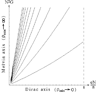
FIG. 2.: Dirac-Melvin contour plot: Lines of constant minimal circumferential radius $\rho_{min}$ range from Dirac line $(\rho_{min}\rightarrow 0)$ up to Melvin line $(\rho_{min}\rightarrow\infty)$.

Taking into account eq.(76), one may further observe that

ρmin≥N3G (82)

and is thus driven to a provocative conclusion: In the presence of gravitation, the Dirac procedure does not make sense. Any attempt to arbitrarily squeeze a magnetic flux tube, while keeping its total magnetic flux fixed, would eventually create a singularity (and close the surrounding space). Magnetic flux simply cannot be confined within flux tubes of sub-Planck cross sections.

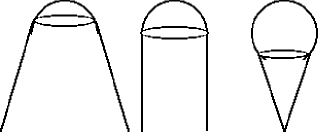
FIG. 3.: The outer space surrounding a cosmic solenoid is conic and open ($\rho\geq\rho_{min}\Rightarrow\gamma\geq 0$) or else closed and singular ($\rho<\rho_{min}\Rightarrow\gamma<0$).

B Dual vector field

In order to decode the Pythagorean quantization condition eq.(78), we restrict ourselves to the London limit of the surface scalar field theory (fixed $\xi=m$). Starting from

$${\cal L}^{S}=-m^{2}\gamma^{ab}\Delta_{a}\Delta_{b}-\Lambda~{},$$ (83)

the $\chi$ equation of motion is

$$J^{a}_{;a}=\frac{1}{\sqrt{-\det\gamma}}\left(\frac{\partial({\cal L}^{S}\sqrt{-\det\gamma})}{\partial\chi_{,a}}\right)_{,a}=0~{}.$$ (84)

The most general solution of this equation is simply

$$J^{a}=\frac{\varepsilon^{abc}}{\sqrt{-\det\gamma}}\partial_{b}q_{c}=\frac{\varepsilon^{abc}}{2\sqrt{-\det\gamma}}f_{bc}~{},$$ (85)

where $f_{ab}\equiv\partial_{[a}q_{b]}$.

One can perform now a Legendre transformation to exchange the scalar phase $\chi$ for a surface vector field $q_{a}$. The prescription then calls for a new Lagrangian

$${\cal L}^{S^{*}}={\cal L}^{S}-J^{a}\chi_{,a}~{},$$ (86)

which up to a total derivative is nothing but

$${\cal L}^{S^{*}}=-\frac{1}{8m^{2}}\gamma^{ab}\gamma^{cd}f_{ac}f_{bd}-e\frac{\varepsilon^{abc}}{\sqrt{-\det\gamma}}A_{a}\partial_{b}q_{c}-\Lambda~{}.$$ (87)

In this dual language, $q_{a}$ has been elevated to the level of a $(2+1)$-dimensional gauge field exhibiting off-diagonal Chern-Simons interaction[13] with the projective electromagnetic gauge field. The corresponding equation of motion is given by

$$f^{ab}_{\hskip 5.0pt;b}=2m^{2}e\frac{\varepsilon^{abc}}{\sqrt{-\det\gamma}}A_{b,c}~{}.$$ (88)

The main question now is the following: What surface gauge configuration is equivalent to $\chi=n\phi$? A simple algebra reveals that the solution consistent with conditions eqs.(III) is

$$f_{tz}=-E=const~{}.$$ (89)

It is accompanied by the relations

$$\displaystyle{j^{\phi}=\frac{eE}{\rho}~{},}$$ (90)

$$\displaystyle{\sigma=\frac{eNE}{\rho}+\frac{E^{2}}{2m^{2}}~{}.}$$ (91)

Now, we match the former eq.(75) with the latter eq.(91) to obtain

$$n-eN=\frac{\rho E}{2m^{2}}~{}.$$ (92)

Notice that the configuration in hand is that of a constant ‘electric’ field in a ‘ring’ capacitor. It is nothing but the closed $(2+1)$-dimensional analog of the $(3+1)$-dimensional plate capacitor. $E$ turns out to be independent of the distance between the $\pm Q$ ‘charges’, normalized such that

$$Q\equiv\frac{\rho E}{2m^{2}e}~{}.$$ (93)

The distance between the ‘charges’ can then be taken to infinity, so that cylindric symmetry is restored without any lose of generality. The resulting generalized quantization condition reads

eΦ2π + 1eQ = n (94)

It is the combination (magnetic flux) + (dual electric charge), rather than the magnetic flux by itself, which gets properly quantized.

The fact that the magnetic flux $N$ does not get quantized comes with no surprise. In theories where the complex field extends to spatial infinity and has non-zero modulus $m$ there, the requirement of finite energy imposes a strict relation between $A_{\mu}$ and the gradient of the phase $\chi$ of the complex field. This relation, in turn, leads to flux quantization because the complex field must be single-valued. The reason that the magnetic flux is not quantized here is that the complex scalar field, to which the projection of $A_{\mu}$ couples minimally, exists only on the solenoid surface and does not extend to spatial infinity.

V Dilaton Gravity

Dilaton gravity usually arises as the low energy limit of string theory, or as the $4$-dimensional effective theory of higher-dimensional Kaluza-Klein gravity. The dilaton is a real scalar field that couples to other fields in a very special way. Two different metrics are often used in dilaton gravity, related to each other by means of a conformal transformation. In the so-called string basis, the dilaton couples to the Ricci scalar associated with the string metric. In the so-called Einstein basis, the dilaton couples only to matter, but does not have a direct gravitational coupling with the Ricci scalar associated with Einstein metric. In this context, it is worth mentioning that the extrinsic curvature surface term prevents the appearance of a dilaton surface term during the conformal transformation. This is why we choose to work here in the Einstein basis, where the self consistent action takes the form

$$Action=\vspace{6pt}$$ (95)

$$-\frac{1}{16\pi}\int_{V_{in}}(e^{-2k\sqrt{G}\eta}g^{\mu\lambda}g^{\nu\sigma}F_{\mu\nu}F_{\lambda\sigma})^{in}\sqrt{-\det g}\,d^{4}x-$$ (96)

$$-\frac{1}{8\pi}\int_{V_{in}}\left(g^{\mu\nu}\eta_{,\mu}\eta_{,\nu}\right)^{in}\sqrt{-\det g}\,d^{4}x+$$ (97)

$$+\frac{1}{16\pi G}\int_{V_{in}}{\cal R}^{in}\sqrt{-\det g}\,d^{4}x-$$ (98)

$$-\frac{1}{8\pi G}\oint_{S}K^{in}\sqrt{-\det\gamma}\,d^{3}y+$$ (99)

$$+\oint_{S}{\cal L}^{S}\sqrt{-\det\gamma}\,d^{3}y-$$ (100)

$$-\frac{1}{8\pi G}\oint_{S}K^{out}\sqrt{-\det\gamma}\,d^{3}y+$$ (101)

$$+\frac{1}{16\pi G}\int_{V_{out}}{\cal R}^{out}\sqrt{-\det g}\,d^{4}x-$$ (102)

$$-\frac{1}{8\pi}\int_{V_{out}}\left(g^{\mu\nu}\eta_{,\mu}\eta_{,\nu}\right)^{in}\sqrt{-\det g}\,d^{4}x+$$ (103)

$$-\frac{1}{16\pi}\int_{V_{out}}(e^{-2k\sqrt{G}\eta}g^{\mu\lambda}g^{\nu\sigma}F_{\mu\nu}F_{\lambda\sigma})^{out}\sqrt{-\det g}\,d^{4}x~{}.$$ (104)

The parameter $k$ is recognized as the dilaton coupling constant; its value depends, however, on the underlying parent theory. It is normalized such that $k=1$ is dictated by string theory, whereas $5$-dimensional Kaluza-Klein theory[14] suggests $k=\sqrt{3}$. The canonical fields are now $g_{\mu\nu}(x)$, $A_{\mu}(x)$, the dilaton $\eta(x)$, and some surface fields as well. We have some idea how do surface fields serve as electromagnetic sources, but the dilaton coupling to the surface fields is still an open question.

Now, in analogy with the previous discussion,

$\bullet$ The variation of the action with respect to $g_{\mu\nu}(x)$ gives rise to the Einstein equations in the entire spacetime

$$\left.{\cal R}_{\mu\nu}-\frac{1}{2}g_{\mu\nu}{\cal R}-8\pi GT_{\mu\nu}\right|_{in/out}=0~{},$$ (105)

and produces the Gauss-Codazzi matching condition on the surface

$$\left.{\cal K}_{ab}\right|_{in}+\left.{\cal K}_{ab}\right|_{out}=8\pi GS_{ab}~{},$$ (106)

only with dilaton modified $T_{\mu\nu}$ and $S_{ab}$.

$\bullet$ The variation of the action with respect to $A_{\mu}(x)$ gives the generalized Maxwell equations in the entire spacetime,

$$\left.{\left(e^{-2k\sqrt{G}\eta}F^{\mu\nu}\right)_{;\nu}}\right|_{in/out}=0~{},$$ (107)

and the junction conditions on the surface modified to include the dilaton factor

$$\begin{array}[]{ccl}&&4\pi\gamma_{ab}j^{b}=\vspace{6pt}\\ &&=\left.e^{-2k\sqrt{G}\eta}F_{\mu\nu}n^{\mu}x^{\nu}_{,a}\right|_{in}+\left.e^{-2k\sqrt{G}\eta}F_{\mu\nu}n^{\mu}x^{\nu}_{,a}\right|_{out}~{}.\end{array}$$ (108)

$\bullet$ The variation of the action with respect to the dilaton field $\eta(x)$ leads to

$$\left.g^{\mu\nu}\eta_{;\mu\nu}+\frac{1}{2}k\sqrt{G}e^{-2k\sqrt{G}\eta}F^{2}\right|_{in/out}=0~{},$$ (109)

and the associated dilaton matching condition

$$\left.n^{\mu}\eta_{;\mu}\right|_{in}+\left.n^{\mu}\eta_{;\mu}\right|_{out}=4\pi\varrho~{}.$$ (110)

The dilaton surface charge $\varrho$ is defined by

$$\varrho=\frac{\partial{\cal L}^{S}}{\partial\eta}-\left(\frac{\partial{\cal L}^{S}}{\partial\eta_{;\mu}}\right)_{;\mu}~{}.$$ (111)

Given the same symmetry constraints, the above equations admit the following solution:

$\bullet$ The inner solution generalizes Melvin universe in a straight forward way

$$ds^{2}_{in}=D^{2}(r)(-dt^{2}+dz^{2}+dr^{2})+\frac{r^{2}}{D^{2}(r)}d\phi^{2}~{},$$ (113)

where

$$D(r)=M(r)^{\frac{1}{1+k^{2}}}=\left(1+\frac{1}{4}GB^{2}r^{2}\right)^{\frac{1}{1+k^{2}}}~{}.$$ (114)

It is accompanied by

$$F_{r\phi}^{in}=\frac{e^{k\sqrt{G}\eta_{0}}}{\sqrt{1+k^{2}}}\frac{Br}{M^{2}(r)}~{},$$ (115)

$$A_{\phi}^{in}=\frac{e^{k\sqrt{G}\eta_{0}}}{\sqrt{1+k^{2}}}\frac{Br^{2}}{2M(r)}~{},$$ (116)

and the dilaton configuration

$$\eta^{in}=\eta_{0}-\frac{k}{\sqrt{G}}\ln{D(r)}~{}.$$ (117)

In accord with $A^{\phi}(0)=0$, it seems reasonable to insist on $\eta_{0}=0$ as well.

$\bullet$ The outer solution has again a flat conic structure

$$ds^{2}_{out}=-dt^{2}+dz^{2}+dr^{2}+\gamma^{2}r^{2}d\phi^{2}~{},$$ (119)

$$F_{r\phi}^{out}=0~{},$$ (120)

$$A_{\phi}^{out}=N~{},$$ (121)

but is furthermore characterized by the constant

$$\eta^{out}\equiv\eta(r\rightarrow\infty)=\eta_{\infty}~{}.$$ (122)

Substituting eqs.(V,V) in eqs.(105-111) and keeping the $g_{\mu\nu}(x)$, $A_{\mu}$, and $\eta(x)$ continuous over the surface, we obtain a bunch of matching conditions:

$$\lambda=\left(1+\frac{1}{4}GB^{2}R_{in}^{2}\right)^{\frac{1}{1+k^{2}}}~{},$$ (124)

$$\gamma=\frac{R_{in}}{R_{out}\left(1+\frac{1}{4}GB^{2}R_{in}^{2}\right)^{\frac{1}{1+k^{2}}}}~{},$$ (125)

$$S^{t}_{t}=S^{z}_{z}=\frac{1}{8\pi G}\left(\frac{1}{R_{out}}-\frac{1}{R_{in}\left(1+\frac{1}{4}GB^{2}R_{in}^{2}\right)^{\frac{1}{1+k^{2}}}}\right)~{},$$ (126)

$$8\pi S^{\phi}_{\phi}=-\frac{1}{1+k^{2}}\frac{B^{2}R_{in}}{\left(1+\frac{1}{4}GB^{2}R_{in}^{2}\right)^{\frac{2+k^{2}}{1+k^{2}}}}~{},$$ (127)

$$N=\frac{1}{\sqrt{1+k^{2}}}\frac{BR_{in}^{2}}{2\left(1+\frac{1}{4}GB^{2}R_{in}^{2}\right)}~{},$$ (128)

$$4\pi j^{\phi}=\frac{1}{\sqrt{1+k^{2}}}\frac{B}{R_{in}\left(1+\frac{1}{4}GB^{2}R_{in}^{2}\right)^{\frac{1}{1+k^{2}}}}~{},$$ (129)

$$-\frac{k}{1+k^{2}}\ln{\left(1+\frac{1}{4}GB^{2}R_{in}^{2}\right)}=\sqrt{G}\eta_{\infty}~{},$$ (130)

$$4\pi\varrho=-\frac{k}{(1+k^{2})}\frac{\sqrt{G}B^{2}R_{in}}{2\left(1+\frac{1}{4}GB^{2}R_{in}^{2}\right)^{\frac{2+k^{2}}{1+k^{2}}}}~{}.$$ (131)

The surface fields are subject to the consistency conditions:

$$S^{t}_{t}=S^{z}_{z}=-\sigma~{},$$ (133)

$$S^{\phi}_{\phi}=-Nj^{\phi}=\frac{\varrho}{k\sqrt{G}}~{}.$$ (134)

Altogether, we can calculate the relevant physical quantities, the conic defect

$$\gamma=\frac{1-8\pi G\sigma R_{in}\left(1+\frac{1}{4}GB^{2}R_{in}^{2}\right)^{\frac{1}{1+k^{2}}}}{\left(1+\frac{1}{4}GB^{2}R_{in}^{2}\right)^{\frac{2}{1+k^{2}}}}~{},$$ (135)

and the circumferential radius of the flux tube

$$\rho=\frac{R_{in}}{\left(1+\frac{1}{4}GB^{2}R_{in}^{2}\right)^{\frac{1}{1+k^{2}}}}~{}.$$ (136)

Eq.(131) tells us that the dilaton surface charge must be different from $0$, therefore the surface fields must couple to the dilaton in some way. The simplest way to do so is to add a dilaton factor in the following way

$${\cal L}^{S}=-e^{l\sqrt{G}\eta}\left(\gamma^{ab}(D_{a}\Phi)^{\dagger}(D_{b}\Phi)+V(\Phi^{\dagger}\Phi)\right)~{}.$$ (137)

The coupling constant $l$ depends on the underlying theory, the character of the field, and the dimension of the surface. Tracing our steps from eq.(66) to eq.(76), we are led to the following relations

$$j^{\phi} = e^{l\sqrt{G}\eta_{\infty}}\frac{2e\Lambda}{n+eN}~{},$$ (138)

$$\sigma = \frac{n}{e}j^{\phi}~{},$$ (139)

$$\varrho = -l\sqrt{G}\sigma~{},$$ (140)

and the subsequent consistency condition

$$\frac{n}{eN}=\frac{k}{l}\geq 1~{}.$$ (141)

Giving both $N$ and $\eta_{\infty}$ seems a bit too much, as the circumferential radius $\rho$ and consequently the conic defect $\gamma$ get fixed. Our current interest, however, is to study $\gamma(N,\rho)$ while holding only $N$ fixed. This way, for each value of $\rho$, in particular $\rho_{min}$, one can calculate the attached $\eta_{\infty}$. Our goal now is to derive the $\rho_{min}$ formula based on the physical requirement $\gamma\geq 0$. We proceed in steps:

$\bullet$ Start by substituting the relation $\displaystyle{j^{\phi}=\frac{e}{n}\sigma}$ into eq.(129) to obtain

$$4\pi\sigma R_{in}\left(1+\frac{1}{4}GB^{2}R_{in}^{2}\right)^{\frac{1}{1+k^{2}}}=\frac{nB}{e\sqrt{1+k^{2}}}~{}.$$ (142)

This enters nicely into the $\gamma=0$ critical condition which now reads

$$1=G\frac{2nB}{e\sqrt{1+k^{2}}}~{}.$$ (143)

$\bullet$ Next, solve eqs.(128,136) to obtain an expression for $B$

$$B=\frac{2N\sqrt{1+k^{2}}}{\rho^{2}}\left(\frac{R_{in}}{\rho}\right)^{k^{2}-1}~{},$$ (144)

which can be used to rewrite the critical condition as

$$1=G\frac{4nN}{e\rho^{2}}\left(\frac{R_{in}}{\rho}\right)^{k^{2}-1}~{}.$$ (146)

To finish the calculation we only need $\displaystyle{\frac{R_{in}}{\rho}}$ as a function of $\rho$ (and the fixed $N$). But such a relation is precisely what eqs.(128,136) are capable of producing, namely

$$\left(\frac{R_{in}}{\rho}\right)^{1+k^{2}}=1+GN^{2}(1+k^{2})\frac{1}{\rho^{2}}\left(\frac{R_{in}}{\rho}\right)^{2k^{2}}~{}.$$ (147)

$\bullet$ The interplay of the two last equations leads us finally to our main result

ρ2min = G4nNe (1-eN4n(1+k2)) 1-k21+k2 (148)

An immediate test of this formula is the recovery of eq.(81) at the $k\rightarrow 0$ limit.

Notice that if the dilaton coupling is such that

$$k^{2}>\frac{4n}{eN}-1>3~{},$$ (149)

there is no lower bound on $\rho$. It is worth mentioning that the class of $(4+D)$-dimensional Kaluza-Klein theories, where the extra dimensions form a $D$-dimensional sphere, induce a $4$-dimensional dilaton gravity characterized by

$$k=\sqrt{1+\frac{2}{D}}~{}.$$ (150)

The maximal value of $k$ happens to be precisely $\sqrt{3}$ (achieved for $D=1$). Thus, in this family of dilaton gravity theories there is always a bound on the circumferential radius of the solenoid.

A final remark is in order. The case $k=1$ is singled out by string theory, and as such deserves special attention. However, in the context of the present work, it does not seem to play any exclusive role in the cosmic solenoid game. One may observe though that the formulae get somewhat simplified, in particular

$$\left.\rho_{min}^{2}\right|_{k=1}=GN^{2}\frac{4n}{eN}~{}.$$ (151)

VI Conclusions

The Dirac procedure of arbitrarily squeezing a magnetic flux tube, while keeping its total flux fixed, is conceptually and substantially modified in the presence of gravity. A given amount of magnetic flux cannot be confined within a Planck-scale cross-section tube without closing the surrounding space and thereby creating a conic singularity. A similar conclusion holds for dilaton gravity (and string theory) as well provided the dilaton coupling is sub-critical.

In this paper, we have constructed a self-consistent general relativistic configuration which describes such a finite cross-section magnetic flux tube. The so-called cosmic solenoid is modeled by an elastic superconductive surface which separates the inner Melvin core from the surrounding flat conic geometry. The Gauss-Codazzi (and electromagnetic) matching conditions are derived by means of a self-consistent action where the source term, which governs the surface currents, is sandwiched between internal and external gravitational surface terms. Surface superconductivity is realized by means of either a complex Higgs scalar minimally coupled to projective electromagnetism, or alternatively by a dual surface gauge field with off-diagonal Chern-Simons interaction with projective electromagnetism. It is surface field theory which dictates the vital connection between surface current and surface energy density, which in turn links the conic defect to the circumferential radius. Our analytic analysis produces a generalized quantization condition, namely

$$(magnetic\,\,flux)+(dual\,\,electric\,\,charge)=integer~{},$$

thereby allowing for a non-trivial Aharonov-Bohm effect.

- [1] Y. Aharonov and D. Bohm, Phys. Rev. 115, 485 (1959).
- [2] P. A. M. Dirac, Proc. Roy. Soc. London A133, 60 (1931).
- [3] D. Kramer, H. Stephani, E. Herlt, and M. MacCallum, Exact Solutions of Einstein’s Field Equations (Cambridge Univ. Press, Cambridge, 1980), p.220-227.
- [4] A. Vilenkin, Phys. Rev. D23, 852 (1981).
- [5] W. Israel, Phys. Rev. D15, 935 (1977); J. R. Gott III, Astrophys. J. 288, 422 (1985); W. A. Hiscock, Phys. Rev. D31, 3288 (1985); B. Linet, Com. Rel. Grav. 17, 1109 (1985).
- [6] E. Copeland, M. Hindmarsh and N. Turok, Phys. Rev. Lett. 58, 1910 (1987); A. Vilenkin and T. Vachaspati. Phys. Rev. Lett. 58, 1041 (1987); D.N. Spergel, T. Piran and J. Goodman, Nucl. Phys. B291, 847 (1987); N.K. Nielsen and P. Olesen, Nucl. Phys. B291, 829 (1987); J.S. Dowker, Phys. Rev. D36, 3095 (1987); V.P. Frolov and E.M. Serebrianyi, Phys. Rev. D35, 3779 (1987); B. Carter, Phys. Lett. B224,61 (1989); M.E.X. Guimaraes and B. Linet, Comm. Math. Phys. 165, 297 (1994); A.A. Tseytlin, Phys. Lett. B346, 55 (1995); J.G. Russo and A.A. Tseytlin, Nucl. Phys. B449, 91 (1995).
- [7] L. Witten, Gravitation: Introduction to Current Research (Wiley, 1962), p.382.
- [8] W.B. Bonnor, Proc. Phys. Soc. London A67, 225 (1954); M. A. Melvin, Phys. Lett. 8, 65 (1964); K.S. Thorne, Phys. Rev. 139, 244 (1965).
- [9] G. W. Gibbons and S. W. Hawking, Phys. Rev. D15, 2752 (1977); J. W. York Jr.,pp. 246-254 in Between Quantum and Cosmos, eds. W. H. Zurek and W. A. Miller (Princeton Univ. Press, Princeton N.J., 1988).
- [10] M.K. Parish and F. Wilczek (gr-qc/9712077).
- [11] W. Israel, Il Nuovo Cim. B44, 1 (1966); A. H. Taub, J. Math. Phys. 21, 1423 (1980); J. Isper and P. Sikivie, Phys. Rev. D30, 712 (1984).
- [12] A. Davidson and K.C. Wali, Nucl.Phys. B349, 581 (1991); J. Garriga and A. Vilenkin, Phys. Rev. D44, 1007 (1991); J. Guven, Phys. Rev. D48, 4604 (1993).
- [13] A. Davidson and E.I. Guendelman, Phys. Lett. B251, 250 (1990); A. Davidson and U. Paz, Phys. Lett. B300, 234 (1993).
- [14] G.W. Gibbons and K. Maeda, Nucl. Phys. B298, 741 (1988); F. Dowker, J.P. Gaunlett, D.A. Kastor and J. Traschen, Phys. Rev. D49, 2909 (1994).