Coherent Line Removal:
Filtering out harmonically related line interference from experimental data, with application to gravitational wave detectors

Abstract

We describe a new technique for removing troublesome interference from external coherent signals present in the gravitational wave spectrum. The method works when the interference is present in many harmonics, as long as they remain coherent with one another. The method can remove interference even when the frequency changes. We apply the method to the data produced by the Glasgow laser interferometer in 1996 and the entire series of wide lines corresponding to the electricity supply frequency and its harmonics are removed, leaving the spectrum clean enough to detect possible signals previously masked by them. We also study the effects of the line removal on the statistics of the noise in the time domain. We find that this technique seems to reduce the level of non-Gaussian noise present in the interferometer and therefore, it can raise the sensitivity and duty cycle of the detectors.

04.80.Nn, 07.05.Kf, 07.50.Hp, 07.60.Ly

I Introduction

In this paper we present a new procedure to remove external interference from the output of gravitational wave detectors. This method allows the removal of phase-coherent lines, not stochastic ones (such as those due to thermal noise), while keeping the intrinsic detector noise. The method works so well that real gravitational wave signals masked by the interference can be recovered.

Our method requires coherence between the fundamental and several harmonics. If there is no such coherence, other methods are available [1, 2, 3], but these methods will remove real signals as well. It is ‘safe’ to apply this technique to gravitational wave data because we expect that coherent gravitational wave signals will appear with at most the fundamental and one harmonic [4]. The information in the harmonics of the interference can be used to removed it without disturbing ‘single-line’ signals. Therefore, this method can be very useful in the search for monochromatic gw signals, such as those produced by pulsars [5, 6].

The method can be used to remove periodic or broad-band signals (e.g., those which change frequency in time), provided their harmonics are sufficient strong and numerous, even if there is no external reference source. The method requires little or no a priori knowledge of the signals we want to remove. This is a characteristic that distinguishes it from other methods such as adaptive noise cancelling (anc) [7], which makes use of an auxiliary reference input derived from one or more sensors. Although in some cases anc can be used without a reference input, it is not clear how anc can, in those cases, cancel harmonics of broad-band signals and at the same time detect weak periodic signals masked by them. This is particularly important in gravitational wave detection, where signals can be as high as 2 kHz while the interference has a fundamental frequency of 50 or 60 Hz.

In this paper, we illustrate the usefulness of this new technique by applying it to the data produced by the Glasgow laser interferometer in March 1996 and removing all those lines corresponding to the electricity supply frequency and its harmonics. As a result the interference is attenuated or eliminated by cancellation in the time domain and the power spectrum appears completely clean allowing the detection of signals that were buried in the interference.

The removal improves the data in the time-domain as well. Strong interference produces a significant non-Gaussian component to the noise. Removing it therefore improves the sensitivity of the detector to short bursts of gw’s.

The rest of the paper is organized as follows. In the next section we define coherent line removal and we give an algorithm for it. In section III we apply the method to remove the 50 Hz harmonics from gw interferometric data. First, we focus our attention to the performance of the algorithm on two minutes of data and we check what happens to a signal masked by the interference. Then, we implement an automatic procedure to clean the whole data stream. We have to solve some difficulties such as the presence of small gaps in the data. We present the results obtained and we show how the electrical interference is completely removed. Moreover, we study the effects of the line removal on the statistics of the noise in the time domain. We compare the mean, the standard deviation, the skewness and the kurtosis of the data before and after the line removal an we also study the Gaussian character. We apply two statistical test to the data: the chi-square test and the Kolmogorov-Smirnov test. Finally, in section IV we discuss the results obtained.

II The principle of Coherent Line Removal

In this section, we define coherent line removal and give an algorithm for it.

We suppose that a certain interference signal $m(t)$ (e.g., 50 Hz interference from the main electricity supply) enters the system. It may already contain harmonics, and non-linear effects in the system electronics may introduce further harmonics. If the processes that produce the harmonics are stationary, then we expect the phase of the harmonics to be simply related to that of $m(t)$. In particular, we assume that the interference has the form

$$y(t)=\sum_{n}a_{n}m(t)^{n}+\left(a_{n}m(t)^{n}\right)^{*}\ ,$$ (1)

where $m(t)$ is a nearly monochromatic function, $n$ are natural numbers, and $a_{n}$ are complex constants that depend on the processes that generate the harmonics, and which are not known a-priori. We suppose that $m(t)$ is a narrow-band function near a frequency $f_{0}$. Then, the $n$th harmonic will be near $nf_{0}$.

The total output of the system also contains noise and possibly other signals. Usually, the data recorded is band-limited, since an anti-aliasing filter is applied to the data before it is sampled. Therefore, the function $y(t)$ must be band-limited as well, and the number of harmonics to be considered is finite. This number, $n_{max}$, is given by the Nyquist frequency and the frequency of the fundamental harmonic $f_{0}$

$$n_{max}=f_{Nyquist}/f_{0}-1\ .$$ (2)

The key to this method is to estimate the interference by using many harmonics of the interference signal and to construct a function

$$h(t)=\sum_{n=1}^{n_{max}}\rho_{n}M(t)^{n}+\left(\rho_{n}M(t)^{n}\right)^{*}\ ,$$ (3)

that is as close a replica as possible of $y(t)$. This function is then subtracted from the output of the system cancelling the interference. If there is a narrow gravitational wave signal within a frequency band obscured by a particular harmonic, it can still be present after line removal, because it will not match the form of the signal being removed. Moreover, because $h(t)$ is constructed from many frequency bands with independent noise, the statistics of noise in any one band are little affected by coherent line removal.

Therefore, we have to design an algorithm to determine the complex function $M(t)$ and all the parameters $\rho_{n}$ that minimize the total output power. Notice that, from the experimental data, we do not independently know the value of the input signal $m(t)$.

As pointed out before, we assume that the data produced by the system is just the sum of the interference plus noise (we ignore here any signals not of the form (1))

$$x(t)=y(t)+n(t)\ ,$$ (4)

where $y(t)$ is given by Eq. (1) and the noise $n(t)$ in the detector is a zero-mean stationary stochastic process. The Fourier transform of the data $\tilde{x}(\nu)$ is simply given by

$$\tilde{x}(\nu)=\tilde{y}(\nu)+\tilde{n}(\nu)\ .$$ (5)

Choosing a subset of harmonics, $\{k\}$, or all of them if one prefers, the idea is to construct the function $M(t)$ by extracting the maximum information from the harmonics considered. The procedure consists in determining the upper and lower frequency limit of each harmonic considered, $(\nu_{ik},\nu_{fk})$, and defining a set of functions $\tilde{z}_{k}(\nu)$ in the frequency domain as

$$\tilde{z}_{k}(\nu)\equiv\left\{\begin{array}[]{cc}\tilde{x}(\nu)&\nu_{ik}<\nu<\nu_{fk}\\ 0&\mbox{elsewhere}\ .\end{array}\right.$$ (6)

Comparing Eq. (6) with (1) and (5) we have

$$\tilde{z}_{k}(\nu)=a_{k}\widetilde{m^{k}}(\nu)+\tilde{n}_{k}(\nu)\ ,$$ (7)

where

$$\tilde{n}_{k}(\nu)=\left\{\begin{array}[]{cc}\tilde{n}(\nu)&\nu_{ik}<\nu<\nu_{fk}\\ 0&\mbox{elsewhere}\ ,\end{array}\right.$$ (8)

is a zero-mean stationary random complex noise. Then, we calculate their inverse Fourier transform

$$z_{k}(t)=a_{k}m(t)^{k}+n_{k}(t)\ .$$ (9)

Since we assume $m(t)$ to be a narrow-band function near a frequency $f_{0}$, each $z_{k}(t)$ is a narrow-band function near $kf_{0}$. It corresponds to one of the harmonics of the external interference plus noise which is independent in the different frequency bands considered ($n_{k}(t)$ for different $k$), since it is produced by an stationary process.

Now, we define

$$B_{k}(t)\equiv\left[z_{k}(t)\right]^{1/k}\ ,$$ (10)

that can be rewritten as

$$B_{k}(t)=(a_{k})^{1/k}m(t)\beta_{k}(t)\ ,$$ (11)

where

$$\beta_{k}(t)=\left[1+{n_{k}(t)\over a_{k}m(t)^{k}}\right]^{1/k}\ .$$ (12)

All these stochastic functions $\{B_{k}(t)\}$ are almost monochromatic around the fundamental frequency, $f_{0}$, but they have different mean values

$$\langle B_{k}(t)\rangle=(a_{k})^{1/k}m(t)\ .$$ (13)

They differ by a certain complex amplitude. In order to estimate the interference $M(t)$, we need to define another set of functions

$$b_{k}(t)\equiv\alpha m(t)\beta_{k}(t)\ ,$$ (14)

such that, these new functions $\{b_{k}(t)\}$ form a set of random variables $-$functions of time$-$ and they all have the same mean value

$$\langle b_{i}(t)\rangle=\alpha m(t)\ .$$ (15)

The functions $b_{k}(t)$ are constructed multiplying the previous functions $B_{k}(t)$ by a certain complex amplitude $\Gamma_{k}$

$$b_{k}(t)=\Gamma_{k}B_{k}(t)\ .$$ (16)

The values of $\Gamma_{k}$ can be obtained from a least square method, comparing the first harmonic considered, $k(1)$, with the other ones (i.e., $\Gamma_{k}$ are the values that minimize $|B_{k(1)}(t)-\Gamma_{k}B_{k}(t)|^{2}$ for each $k$). We find

$$\Gamma_{k}=\sum_{j}B_{k(1)}(j\Delta t)B_{k}(j\Delta t)^{*}{\Big{/}}\sum_{j}|B_{k}(j\Delta t)|^{2}\ ,$$ (17)

where $\Delta t$ corresponds to the time interval between two samples, so that the sampling frequency is equal to $1/\Delta t$, $*$ denotes the complex conjugate, and the index $j$ counts sampled points in the time domain.

Now, we want to construct $M(t)$ as a function of all $\{b_{k}(t)\}$, in such a way that it has the same mean and minimum variance. If we assume the function $M(t)$ to be linear with $\{b_{k}(t)\}$, statistically the best estimate is

$$M(t)=\left(\sum_{k}{b_{k}(t)\over{\rm Var}[\beta_{k}(t)]}\right){\Big{/}}\left(\sum_{k}{1\over{\rm Var}[\beta_{k}(t)]}\right)\ .$$ (18)

The variance of $\beta_{k}(t)$ can be estimated by doing a Taylor expansion of equation (12), hence we obtain

$${\rm Var}[\beta_{k}(t)]={\langle n_{k}(t)n_{k}(t)^{*}\rangle\over k^{2}|a_{k}m(t)^{k}|^{2}}+\mbox{corrections}\ ,$$ (19)

where we can approximate

$$|a_{k}m(t)^{k}|^{2}\approx|z_{k}(t)|^{2}\ ,$$ (20)

and the numerator can be rewritten as

$$\langle n_{k}(t)n_{k}(t)^{*}\rangle=\int d\nu\int d\nu^{\prime}\langle\tilde{n}_{k}(\nu)\tilde{n}_{k}(\nu^{\prime})^{*}\rangle e^{2\pi i(\nu-\nu^{\prime})t}\ .$$ (21)

In the case of stationary noise (i.e., $\langle\tilde{n}(\nu)\tilde{n}(\nu^{\prime})^{*}\rangle=S(\nu)\delta(\nu-\nu^{\prime})$), the previous equation becomes

$$\langle n_{k}(t)n_{k}(t)^{*}\rangle = \int d\nu\int d\nu^{\prime}\,S_{k}(\nu)\delta(\nu-\nu^{\prime})e^{2\pi i(\nu-\nu^{\prime})t}$$ (22)

$$= \int_{\nu_{ik}}^{\nu_{fk}}S(\nu)d\nu\ ,$$ (23)

where $S(\nu)$ is the power spectral density of the noise.

After we have estimated the interference $M(t)$, it only remains to determine the parameters $\rho_{n}$ in Eq. (3). They can be obtained by minimizing the total output power in the time domain, $|x(t)-h(t)|^{2}$ (i.e., applying a least square method). Taking into account that the noise near the different harmonics is uncorrelated, it yields

$$\rho_{n}=\sum_{j}x(j\Delta t)M^{n}(j\Delta t)^{*}{\Big{/}}\sum_{j}|M^{n}(j\Delta t)|^{2}\ ,$$ (24)

which is the form we use in our algorithm. One can also minimize the total output power in the frequency domain, $|\tilde{x}(\nu)-\tilde{h}(\nu)|^{2}$. Then, we get

$$\rho_{n}=\sum_{j}\tilde{x}(j\Delta\nu)\widetilde{M^{n}}(j\Delta\nu)^{*}{\Big{/}}\sum_{j}|\widetilde{M^{n}}(j\Delta\nu)|^{2}\ ,$$ (25)

where $j$ is now the frequency index.

III Removal of 50 Hz harmonics from interferometric data stream

In this section, we present experimental results that demonstrate the performance of the coherent line removal and show its potential value. This new technique is applied to the data produced by the Glasgow laser interferometer and the electrical interference is successfully removed.

In the study of the data produced by the Glasgow laser interferometer in March 1996 [8], we observe in the spectrum many instrumental lines, some of them at multiples of 50 Hz. All these lines are rather broad, and when we compare them, we observe that their overall structure is very similar but only the scaling of the width is different (see figure 1).

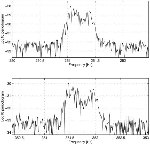
FIG. 1.: Comparison of the structure of the lines at 250 Hz and at 350 Hz of the power spectrum (of 2 minutes) of the Glasgow data. The broad shape is due to the wandering of the incoming electricity frequency.

If we look at these lines in more detail, in smaller length Fourier transform (seconds in length), they appear as well defined small bandwidth lines which change frequency over time in the same way, while other ones remain at constant frequency. Therefore, all these lines at multiples of 50 Hz must be harmonics of a single source (for example the electricity supply), and this makes them good candidates to test our algorithm.

The same phenomenom is observed in the Garching 30-meter prototype [9]. The LIGO group has also reported largely instrumental artifacts at multiples of the 60 Hz line frequency in their 40-meter interferometer [10]. Therefore, this seems to be a general effect present in the different prototype interferometers.

In the Glasgow data, the lines at 1 kHz have a width of 5 Hz. Therefore, we can ignore these sections of the power spectrum or we can try to remove this interference in order to be able to detect gw signals masked by them.

In the large-scale detectors now under construction, we expect the amount of interference to be smaller. Prototypes like the Glasgow instrument were designed to test optical systems, not to collect high quality data, and the effort required to exclude interference was not justified by the goals of the prototype development. However, we cannot be sure that such interference will be completely absent or that other sources of interference will not manifest themselves in long-duration spectra. Indeed, the Glasgow data [8] contain other regular features of unknown origin [11]. For this reason we investigate a solution to this problem using the existing data.

A Testing procedure

As a first test, we apply the coherent line removal to a set of $2^{19}$ points (approximately two minutes) of the Glasgow data. The stretch of data selected corresponds to a period of time in which the detector is on lock and the level of noise is low.

After calculating the DFT of this piece of data (using the FFT algorithm), we notice that the odd harmonics of the 50 Hz line are much stronger than the even ones. Thus, in order to construct the reference wave-form $M(t)$, we choose a set of ten harmonics $k=\{3,5,7,\ldots,21\}$, corresponding to the lines at frequencies $50\times k(i)$ Hz. We also give as inputs the corresponding upper and lower frequency limits of each of these harmonics, $(\nu_{ik},\nu_{fk})$, that are obtained from the power spectrum.

The first difficulty that arises is to estimate the power spectral density (psd) of the noise (without the external electrical interference) in those frequency bands corresponding to the harmonics considered. In the absence of any extra information, we assume the psd is constant in each frequency band and we calculate its value by averaging the psd in the nearness of the line considered. With all this information, we apply the line removal and we successfully remove the electrical interference as it can be seen in figure 2.

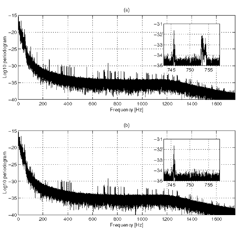
FIG. 2.: Decimal logarithm of the periodogram of $2^{19}$ points (approximately 2 minutes) of (a) the Glasgow data with the detail of one of the harmonics near 754 Hz. (b) The same data after the removal of the electrical interference as described in the text.

We have repeated the procedure considering only six harmonics, $k=\{3,5,7,9,11,13\}$ and, surprisingly, the interference still remains below the noise level showing the power of this algorithm. The method requires further study (i.e., with simulated noise and different signals) in order to characterize how its performance depends upon the number of harmonics and their strength. Of course, in order to obtain a minimum variance for $M(t)$, the larger number of harmonics considered the better. The minimum number of harmonics required depends, in each case, on the strength of the harmonics considered, more precisely, with the ratios $\langle n_{k}(t)n_{k}(t)^{*}\rangle/|a_{k}m(t)^{k}|^{2}$, appearing in equation (19), which should be smaller than one.

Now, we are interested in studying what will happen to a signal masked by the interference. For this purpose, we apply coherent line removal to the true experimental data with an external simulated signal at 452 Hz, that is initially hidden due to its weakness.

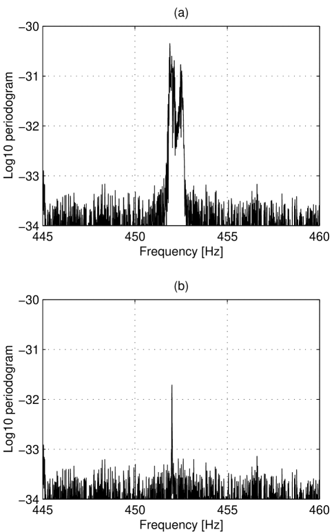
FIG. 3.: (a) Zoom of the same experimental data as in figure 2 with an artificial signal added at 452 Hz. (b) The data in (a) after removing the electrical interference, revealing that the signal remains detectable.

First, we take into account not to consider the harmonic near 450 Hz as an input to estimate the interference $M(t)$. In this case, we succeed in removing the electrical interference while keeping the signal present in the data, obtaining a clear outstanding peak over the noise level and whose amplitude is not modified (see figure 3).

However, now we apply the same procedure, but including the harmonic near 450 Hz ($k=9$). In this case, $M(t)$ contains a low-level of signal component in addition to the electrical interference. This signal component causes a cancellation of the $25.4\ \%$ of the amplitude of the line at 452 Hz and also the appearance of weaker signals under the other harmonics. The amount of signal distortion depends basically on the variance of $\beta_{9}(t)$ with respect to the other ones.

Any of the harmonics considered in the construction of the reference function $M(t)$ may contain a ‘single-line’ signal we want to recover, but a-priori, we will not be able to say which one is masking a signal. The key is that gravitational wave signals will not be present with multiples harmonics. Therefore, after applying the line removal, we will have a candidate line. If we are interested, we can repeat the procedure without using the “dangerous” harmonic and hence, we can make use of the whole power of the algorithm. With this aim, it is better to consider the lower harmonics, since their frequency bands are narrower and also the probability of having a thermal line buried with them may accordingly be lower.

B Automatic cleaning of whole data stream

The next step consists in removing the electrical interference from the whole data stream making use of an automatic procedure.

The Glasgow data consist of 19857408 points, sampled at 4 kHz and quantized with 12 bit analog-to-digital converter with a dynamical range from -10 to 10 Volts. The data are divided into 4848 blocks of 4096 points. For each of these blocks, the standard deviation is calculated and, depending whether it exceeds a certain value, the whole block is classified as “bad”.

The first 18 minutes of data are rendered useless due to a failure of autolocking. Therefore, we decide to ignore the first 1153 blocks. The rest of the data are separated into groups of 64 blocks (approximately one minute of data) and, for each of them, the coherent line removal algorithm is applied.

The first difficulty that arises is how to deal with the “bad” blocks. In some cases, the detector is out of lock and, in other ones, the level of noise is very high. Since this method is based on Fourier transforms, the suggestion of defining a window function that vetoes the “bad” data produces that each real feature in the spectrum be accompanied by horrible side lobes and satellites features, the structure of which depends in detail on the distribution of those gaps. In order to reduce these effects, we realize that it is better not to remove the “bad” data, but to divide each “bad” block by its standard deviation. Of course, the “bad” blocks are not taken into account in order to determine the parameters $\rho_{n}$ given by Eq. (24). This is done multiplying the function $M(t)$ and the input data by a window function, such that, it is equal to zero for each block of “bad” data and one otherwise. As a result, all “bad” data are set to zero in the output.

Another important issue is to design an strategy to detect the harmonics of the electricity supply interference, and determine their upper and lower frequency limits without interacting with the program. This is not an easy task, since the noise level is very high, the lines are broad, they vary in time, and they are partially hidden by the noise. Also, the presence of violin modes closed to the harmonics, or completely overlapping with them, makes it more difficult.

The method we have used consists in computing the power spectrum for each piece of the data (with the electrical interference) and we search for the location of the first harmonic considered. We calculate the mean, $m_{k(1)}$, and the standard deviation, $\sigma_{k(1)}$, in a certain frequency interval which we are sure contains the first harmonic. Then, we search in detail for ten harmonics in the frequency bands centered respectively at $m_{k(1)}k(i)/k(1)$ and which amplitudes are proportional to $\sigma_{k(1)}k(i)/k(1)$. In each band, we set a threshold depending on the mean and the variance of the power spectrum at the ends of those intervals. We determine the points which are over the threshold, and from them, we try to determine the nearest points to the beginning and end of the corresponding line. One has to be careful, since violin modes (i.e., the transverse modes of the suspension wires) can be present and stand out of the threshold, and also, the harmonics considered can be partially under it.

Our criteria consists in lowering the threshold until there is a certain minimum number of points over it. This number is set depending on the length of the data (number of blocks used) and the harmonic considered. Then, we find the location of, not the first but, a certain $n$-point, $p(n)$, that stands out of that threshold and we consider the first point of the line to be $p(n)-n$. A similar procedure is applied for the last point. In case that there is just one signal present in this interval, we would expect $p(n)-n$ to be similar to $p(1)$, but in case that, for example, a violin mode is very close to the harmonic (but not overlapping with it), then we hope that the quantity $p(n)-n$ would lie between the two lines. Finally, the initial and final points are shifted until they reach a local minimum of an averaged power spectrum.

Solved these two questions, we execute our program using MATLAB software running on an SGI–Origin 2000 and, after approximately 140 minutes CPU time, the data is stored almost clean of electrical interference.

To show the result of the program, in figure 4, we compare a zoom of the spectrogram for the frequency range between 740 and 760 Hz. There, we can see the performance of the coherent line removal algorithm, comparing how a line due to an harmonic of the electrical interference in the initial data is removed. We notice that the algorithm did not work properly for two sets of blocks: 1730-1793 and 3213-3276. In both cases, this is caused by the presence of a huge number of “bad” blocks corresponding to periods in which the detector is out of lock.

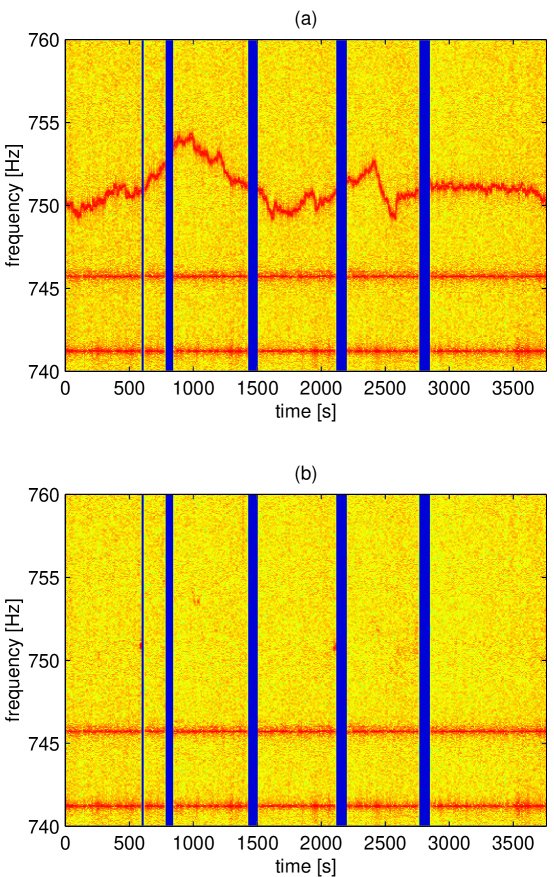
FIG. 4.: Comparison of a zoom of the spectrogram. The dark areas correspond to the periods in which the detector is out of lock. (a) is obtained from the Glasgow data. We can observe the wandering of the incoming electrical signal. The other two remaining lines at constant frequency correspond to violin modes. (b) The same spectrogram as in (a) after applying coherent line removal, showing how the electrical interference is removed to below the noise level.

In order to reduce the noise variance and see the quality of the performance of the coherent line removal, we calculate an average periodogram using Welch’s overlap method [12, 13]. We remove the two sets of bad data, we divide the rest into sets of 128 blocks with overlaps of 64 blocks, and we average over the short periodograms. By doing so, we observe how the harmonics of the electricity supply frequency still remain undetectable over the noise level. Also, we discover a series of thin features at 701, 1002 and 1503 Hz, and the presence of violin modes at 853, 1451 and 1750 Hz that were buried with the electrical interference before.

C Effects on the statistics

After removing the electrical interference, we are interested in studying possible side effects on the statistics of the noise in the time domain.

For both sets of data, we calculate the mean, the standard deviation, the skewness and the kurtosis of each block, and we compare the values obtained. We observe that the mean is hardly changed and its value is almost constant around $-0.018\pm 0.002$ Volts for the “good” blocks. By contrast, a big difference is obtained for the standard deviation. In the Glasgow data, we see that the standard deviation is not uniform, it tends to increase, specially during an on lock period until the detector goes out of lock and its average value is around $1.50$ Volts. After the line removal, we observe the same behavior, but for each block, the standard deviation is reduced by $0.45\pm 0.05$ Volts, obtaining an average value around $1.05$ Volts (see figure 5).

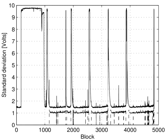
FIG. 5.: The solid line (top one) corresponds to the block standard deviation of the Glasgow data. When the detector in on lock, its typical value is $1.50$ Volts. However, when the detector is out of lock, this value grows up to 10. The dashed line (bottom one) corresponds to the standard deviation of the data after removing the electrical interference. Its typical value is now around $1.05$ Volts.

The skewness characterizes the degree of asymmetry of the distribution around its mean. The value for each block changes from $-0.015\pm 0.060$ in the original Glasgow data, to $-0.005\pm 0.040$ after the line removal. The kurtosis measures the relative peakedness or flatness of a distribution with respect to a normal distribution. In both sets of data, the kurtosis fluctuates from a slight negative value to a large positive one. For the Glasgow data, the kurtosis is concentrated around $-0.35\pm 0.15$, obtaining a maximum (isolated) value of $7.8$, and after removing the electrical interference, it is around $-0.15\pm 0.15$. Therefore, it is much closer to the zero value, even though the (isolated) spikes are larger, the highest value being $16.7$. The kurtosis value gives an idea how Gaussian the noise is and whether it has a large tail or not. A value near zero suggests a Gaussian nature, and a positive value indicates that the distribution is quite peaked. Since both values, the skewness and the kurtosis, are getting closer to zero after the line removal, we are interested in studying the possible reduction of the level of non-Gaussian noise. To this end, we choose a set of $410$ blocks of “good” data and we study their histogram, calculating the number of events that lie between different equal intervals, before and after removing the electrical interference.

Instead of plotting the number of events versus its location, we plot their logarithm as a function of $(x-\mu)^{2}$, where $x$ is the central position of the interval considered and $\mu$ is the mean (see figure 6). In case that the noise distribution resembles a Gaussian, all points should fit on a straight line of slope $-1/2\sigma^{2}$, where $\sigma$ is the standard deviation. We observe that this is not the case. Although, both distributions seem to have a linear regime, they present a break and then a very heavy tail. The two distributions are very different. This is mainly due to the change of the standard deviation, that has a value of $\sigma_{G}=1.5151$ Volts for the original Glasgow data and $\sigma_{c}=1.0449$ Volts after removing the interference.

We can zoom the ‘linear’ regime and change the scale in the abscissa to $(x-\mu)^{2}/(2\sigma^{2})$. Then, any Gaussian distribution should fit into a straight line of slope -1. We observe that after removing the interference, it follows a Gaussian distribution quite well up to $4\sigma$. Whereas, the original Glasgow data does not fit to a straight line: The slope changes; it does not correspond to the right one; and close to the origin, it is flatter than a Gaussian due to the negative kurtosis value.

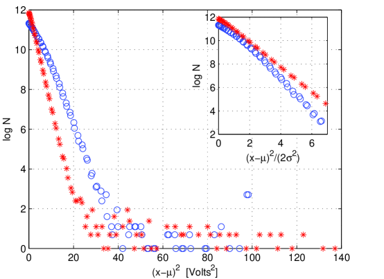
FIG. 6.: Comparison of the logarithm plot of the histogram for the blocks 4111 to 4520 as a function of $(x-\mu)^{2}$. The circles correspond to the Glasgow data and the stars to the same data after removing the electrical interference. The Glasgow data is characterized by $\mu=-0.0182$ Volts and $\sigma=1.5151$ Volts. After the line removal, we obtain the values of $\mu=-0.0182$ Volts and $\sigma=1.0449$ Volts. In the right-hand corner, there is zoom of the original figure, but rescaled so that the abscissa corresponds to $(x-\mu)^{2}/2\sigma^{2}$. If the data resembles a Gaussian distribution, we will expect a single straight line of slope -1. This is not the case for the Glasgow data, but it seems to be satisfied for the clean data up to $4\sigma$. The large number of points in the highest bin of the Glasgow data is an effect of saturating the ADC. These points are spread to higher and lower voltages by line removal.

We can study the population of the noise in the tail of the distributions and see how it is affected by the line removal. The number of events that exceeds the $\pm 7$ Volts is of 60 in the Glasgow data and of 51 after removing the interference, meaning that the events are now concentrated at lower voltages. But, one can be more interested in comparing the number of events that exceeds a certain standard deviation value. The population outstanding $5\sigma$ is just 51 for the Glasgow data, but of 96 after the line removal. This higher number of events in the tail is due to the big reduction of the standard deviation value, since the same $\sigma$ value corresponds to a much lower voltage.

The Glasgow data has a dynamical range from $-10$ to $+10$ Volts, as it was defined by the computer board they use. After removing the electrical interference, we observe events at 11.8 Volts. This implies that the amplitude of the signal we remove is of at least 1.8 Volts. This high signal amplitude, together with the previous existence of events close to the limit of the dynamical range allowed, and the decrease of the standard deviation can explain how, in some ‘isolated’ cases, the kurtosis value grows so much.

In order study the Gaussian character, we apply two statistical tests to the data: the chi-square test [14] that measures the discrepancies between binned distributions, and the one-dimensional Kolmogorov-Smirnov test [15] that measures the differences between cumulative distributions of a continuous data. Both tests can be applied to our data since we can always turn continuous data into binned data, by grouping the events into specified ranges of the continuous variable.

We compute the significance probability for each block of the data using both tests and we check whether the distribution are Gaussian or not. The two tests are not equivalent but in any case, the values of the significance probability would be close to unity for distribution resembling a Gaussian distribution (see figures 7 and 8).

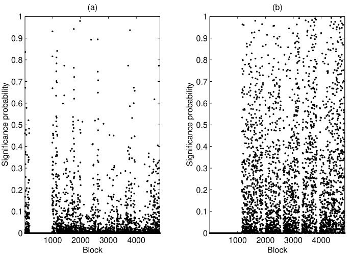
FIG. 7.: Comparison of the block chi-square test: (a) for the Glasgow data, (b) after the removal of the interference.

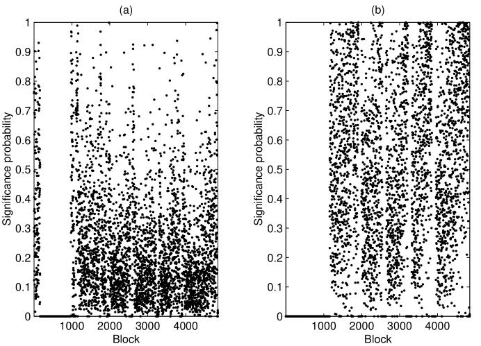
FIG. 8.: Block Kolmogorov-Smirnov test: (a) for the Glasgow data, (b) after the removal of the interference.

In all cases, we find that the data deviates from a Gaussian distribution by a wide margin. Although, for some blocks we get a high significance probability, this cannot be taken as the dominant trend. As a result of both tests, we note how the significance probability increases after removing the electrical interference, showing that this procedure suppresses some non-Gaussian noise, although, generally speaking, the distribution may still be described as being non-Gaussian in character.

IV Discussion

We have described a new exciting technique for removing troublesome interference from external coherent signals (such as the electricity supply frequency and its harmonics) which can obscure wide frequency bands. This approach can leave the spectrum clean enough to see true gravitational waves that have been buried in the interference. Therefore, this new method appears to be good news as far as searching for continuous waves is concerned.

We have applied coherent line removal to the Glasgow laser interferometer data and we have succeeded in removing the electrical interference. By doing so, we have discovered some new thin features at 701, 1002 and 1503 Hz, and also some violin modes at 853, 1451 and 1750 Hz that were masked by the interference in the original data.

The results of the previous section indicate that coherent line removal can also reduce the level of non-Gaussian noise. This result is very encouraging for large-scale interferometers. Nicholson et al. [16] reported that the effective strain sensitivity in coincident observations for short bursts in the time scale, was a factor of 2 worse than the theoretical best limit that the detectors could have set, the excess being due to unmodeled non-Gaussian noise, and they also indicate that reducing this non-Gaussian noise could raise the sensitivity and duty cycle of working detectors close to their optimum performance.

Coherent line removal can be applied to any kind of coherent interference signal. It only requires phase-coherence between the fundamental and several harmonics. Since the algorithm can be applied recursively for small pieces of a long data stream, the global physical process that produces the interference (and all the harmonics) does not need to be stationary, i.e., the parameters $a_{n}$ in Eq. (1) may change in time. We only require that the process could be considered stationary for those time scales in which the algorithm is applied. For every small piece of data, the reference function $M(t)$ and all the parameters $\rho_{n}$ are calculated allowing any possible changes. This method can be considered as an adaptive method that has the ability to adjust its own parameters automatically and requires little knowledge of the signal we want to remove.

Coherent line removal may have more applications, not only for the detection of gw radiation, but also, for example, in radioastronomy or in other completely different fields.

We hope that the results described before will encourage others in testing and applying this new technique to other problems.

REFERENCES

- [1] Allen B., 1997, GRASP: a data analysis package for gravitational wave detection, manual version 1.5.0. University of Wisconsin-Milwaukee
- [2] Thomson D.J., 1982, Spectrum Estimation and Harmonic Analysis in Proceedings of the IEEE, 70, 1055-96
- [3] Percival D.B., Walden A.T., 1993, Spectral analysis for physical applications, first edition, Cambridge University Press
- [4] Bonazzola S., Gourgoulhon E., 1996, Astron. Astrophys. 312, 675-690
- [5] Schutz B.F., 1997, eds. Marck J.A. & Lasota J.P., in Relativistic Gravitation and Gravitational Radiation. Cambridge University Press, Cambridge
- [6] Thorne K.S., 1995, eds. Kolb E.W. & Peccei R., in Proceedings of Snowmass 1994 Summer Study on Particle and Nuclear Astrophysics and Cosmology. World Scientific, Singapore, p. 398
- [7] Widrow B., Glover J.R., McCool J.M., Kaunitz J., Williamns C.S., Hearn R.H., Zeidler J.R., Dong E., Goodlin R.C., 1975, Adaptive Noise Cancelling: Principles and Applications in Proceedings of the IEEE, 63, 1692-1716
- [8] Jones G.S., 1996, Fourier analysis of the data produced by the Glasgow laser interferometer in March 1996, internal report, Cardiff University, Dept. of Physics and Astronomy
- [9] Maischberger K., Ruediger A., Schilling R., Schnupp L., Winkler W., Leuchs G., 1991, Status of the Garching 30 meter prototype for a large gravitational wave detector eds. P.F. Michelson, En-Ke Hu & G. Pizzella, in Experimental Gravitational Physics. World Scientific, Singapore, 316-21
- [10] Abramovici A., Althouse W., Camp J., Durance D., Giaime J.A., Gillespie A., Kawamura S., Kuhnert A., Lyons T., Raab F.J., Savage Jr. R.L., Shoemaker D., Sievers L., Spero R., Vogt R., Weiss R., Whitcomb S., Zucker M., 1996, Physics Letters A 218, 157
- [11] Królak A., 1997, Searching data for periodic signals, in proceedings of the 2nd workshop on Gravitational Wave Data Analysis. Orsay, France
- [12] Welch P.D., 1967, The Use of Fast Fourier Transform for the Estimation of Power Spectra: A Method Based on Time Averaging Over Short, Modified Periodograms, in IEEE Trans. Audio Electroacoust. AU-15, 70-73
- [13] Kay S., 1988, Modern Spectral Estimation. Englewood Cliffs, Prentice-Hall, NJ
- [14] Bendat J.S., Pierso A.G., Random data analysis and measurements procedures. John Wiley & Sons
- [15] Stuart A., Ord K., 1994, Kendall’s Advanced Theory of Statistics, vol. 1. Edward Arnold. London
- [16] Nicholson D., Dickson C.A., Watkins W.J., Schutz B.F., Shuttleworth J., Jones G.S., Robertson D.I., Mackenzie N.L., Strain K.A., Meers B.J., Newton G.P., Ward H., Cantley C.A., Robertson N.A., Hough J., Danzmann K., Niebauer T.M., Rüdiger A., Schilling R., Schnupp L., Winkler W., 1996, Physics Letters A 218, 175-180