Canonical Quasilocal Energy and Small Spheres

Abstract

Consider the definition $E$ of quasilocal energy stemming from the Hamilton-Jacobi method as applied to the canonical form of the gravitational action. We examine $E$ in the standard “small-sphere limit,” first considered by Horowitz and Schmidt in their examination of Hawking’s quasilocal mass. By the term small sphere we mean a cut $S(r)$, level in an affine radius $r$, of the lightcone $N_{p}$ belonging to a generic spacetime point $p$. As a power series in $r$, we compute the energy $E$ of the gravitational and matter fields on a spacelike hypersurface $\Sigma$ spanning $S(r)$. Much of our analysis concerns conceptual and technical issues associated with assigning the zero-point of the energy. For the small-sphere limit, we argue that the correct zero-point is obtained via a “lightcone reference,” which stems from a certain isometric embedding of $S(r)$ into a genuine lightcone of Minkowski spacetime. Choosing this zero-point, we find the following results: (i) in the presence of matter $E={\textstyle\frac{4}{3}}\pi r^{3}[T_{\mu\nu}u^{\mu}u^{\nu}]|_{p}+{\rm O}(r^{4})$ and (ii) in vacuo $E={\textstyle\frac{1}{90}}r^{5}[T_{\mu\nu\lambda\kappa}u^{\mu}u^{\nu}u^{\lambda}u^{\kappa}]|_{p}+{\rm O}(r^{6})$. Here, $u^{\mu}$ is a unit, future-pointing, timelike vector in the tangent space at $p$ (which defines the choice of affine radius); $T_{\mu\nu}$ is the matter stress-energy-momentum tensor; $T_{\mu\nu\lambda\kappa}$ is the Bel-Robinson gravitational super stress-energy-momentum tensor; and $|_{p}$ denotes “restriction to $p$.” Hawking’s quasilocal mass expression agrees with the results (i) and (ii) up to and including the first non-trivial order in the affine radius. The non-vacuum result (i) has the expected form based on the results of Newtonian potential theory.

Introduction

Consider Einstein’s non-covariant first-order action[1], the 4-integral of a “bulk” Lagrangian which is quadratic in the Christoffel symbols and thus often called the “$\Gamma\Gamma$ action.” Starting with the Einstein action, one applies standard techniques associated with Noether’s theorem in order to derive, among other things, an energy definition in general relativity: namely, the 2-integral of an Einstein superpotential over some generic 2-surface $S$ in spacetime $M$. The Einstein energy is well known to be ambiguously defined because it depends on the choice of background coordinates. Nevertheless, one may use the Einstein construction to define sensible notions of total gravitational energy. Indeed, consider the scenario of asymptotic flatness, say, towards future null infinity $J^{+}$. In this case, $S$ tends to a round, infinite-radius, 2-sphere cut of $J^{+}$, and the (now suitably unique) choice of asymptotically Cartesian coordinates ensures that the Einstein energy agrees with the accepted Trautman-Bondi-Sachs (tbs) notion of total energy.[2] However, were we to offer the Einstein definition as the energy contained within some quasilocal (that is, finite) 2-surface $S$, we would still be confronted with the task of choosing a physically meaningful set of background coordinates. The only natural choice would be coordinates which are partially adapted to the embedding of $S\subset M$. However, such a choice wrecks the agreement between the Einstein and tbs energies as $S$ tends towards $J^{+}$. In fact, choosing such $S$-adapted coordinates, one finds that the Einstein energy blows up in the said limit. Similar statements can be made regarding other approaches for defining energy, which trade coordinate (that is, holonomic-frame) ambiguity for ambiguity of a different stripe, e. g. tetrad (or rigid) frame, spin frame, or auxiliary vector (or spinor) fields. The traditional party line regarding these issues is the following: there is no over-arching rule, applicable for all quasilocal 2-surfaces, for selecting a (suitably unique) background frame; whence gravitational quasilocal energy is not well-defined. To what extent does the stubborn presence of frame ambiguity in the quasilocal context point to a gap in our understanding of gravitational energy? To address this question and sharpen our thoughts on these issues, let us consider a covariant version of the Einstein construction.

Employing a straightforward field-theoretic generalization of the Hamilton-Jacobi (hj) method[5], one may derive from a covariant action functional an expression for canonical quasilocal energy (qle) in general relativity.[6] We call this definition of qle canonical, because, owing to its intimate connection with hj theory, this qle is also the on-shell value of the gravitational Hamiltonian for the choice of unit lapse function and vanishing shift vector at the system boundary.[6] We also note that the canonical qle is the thermodynamic internal energy in a thermodynamical description of a (relativistic) self-gravitating system.[7] The analysis that leads to the canonical qle runs along a somewhat different line than the one followed in a Noether-type analysis, but it also leads to a concept of energy which is not unique. Indeed, as is always the case with energy, the canonical qle is defined only up to the choice of a zero-point. The zero-point ambiguity may be traced to a freedom present in the action principle. Namely, one may always add to the action any functional of the fixed boundary data without affecting the variational principle. As with the situation above, if the goal is to obtain agreement with the accepted notions of gravitational energy at spacelike or null infinity, then there is a suitably unique choice of energy zero-point[6, 8], whereas at the quasilocal level there seems to be no preferred choice. While at first sight this seems no better or worse than the situation encountered above, notice that now the ambiguity in the energy has a physical interpretation, and, moreover, is a field-theoretic generalization of the standard ambiguity present in the hj definition of energy in ordinary mechanics. We may now restate the emphasized portion of the party line above as follows: there is no over-arching rule, applicable for all quasilocal 2-surfaces, for selecting a (suitably unique) zero-point. Taking this statement at face value, we claim that it is the physicist’s job to select an appropriate energy zero-point, guided by the principle that the selection should be appropriate for the physics of the problem at hand. We would like to point out that this is a common enough state of affairs in general relativity, a many-faceted theory known for its wealth of possible boundary conditions. Indeed, by way of analogy consider the search for solutions of the Einstein field equations. In practice, relativists certainly do not attempt to find the general solution, rather they attempt to find solutions given some additional physical input (boundary conditions, symmetries, etc.). In practice, the same such additional input is needed to associate a meaningful qle with a particular quasilocal 2-surface.

Bearing these points in mind, we recall the form of the canonical qle:

$$E=(8\pi)^{-1}\int_{S}{\rm d}S\left(k-k|^{\rm{\scriptscriptstyle ref}}\right){\,},$$ (1)

where we adopt geometrical units (in which both Newton’s constant and the speed of light are set to unity), $S$ is a closed 2-surface, ${\rm d}S$ is the proper area element on $S$, and $k$ is the mean curvature of $S$ as embedded in a spanning 3-surface $\Sigma$. It is important to realize that this $E$, while obtained as a proper surface integral over $S$, is the energy of the gravitational and matter fields which live on $\Sigma$, that is to say, $E$ is a functional of the initial data of $\Sigma$. This concept of energy is rooted in the $3+1$ view of spacetime geometry, and for a fixed $S$ it is slightly sensitive to the choice of spanning $\Sigma$. [More precisely, $E$ depends on the equivalence class of spanning 3-surfaces determined by a unit timelike vector on (and pointing orthogonal to) $S$.] This sensitivity is quite analogous to the observer dependence of energy in special relativity, and a priori we expect its presence.[9] In general, the term $k|^{\rm{\scriptscriptstyle ref}}=k|^{\rm{\scriptscriptstyle ref}}(\sigma_{ab})$ represents an arbitrary (local) function of the intrinsic metric $\sigma_{ab}$ of $S$ and corresponds to the freedom to assign the qle zero-point. Notice that this freedom corresponds to a proper surface integral of what is effectively a free function of two variables. This freedom, stemming from the field-theoretic character of gravity, is rather more subtle than the freedom in simple mechanics of simply adding a constant to the energy. For our analysis here we only consider two energy zero-points, one determined by lightcone reference and the other by Euclidean reference. We make these concepts precise below.

In this paper we examine the canonical qle in the standard “small-sphere limit,” first considered by Horowitz and Schmidt in their classic examination of Hawking’s quasilocal mass. By the term small sphere we mean a cut $S(r)$, level in an affine radius $r$, of the lightcone $N_{p}$ belonging to a generic spacetime point $p$. As a power series in $r$, we compute the energy $E$ of the gravitational and matter fields on a spacelike hypersurface $\Sigma$ spanning $S(r)$. Much of our analysis concerns conceptual and technical issues associated with assigning the zero-point of the energy, and, therefore, particularly elucidates the points raised in the first two paragraphs above. For the small-sphere limit, we argue that the correct zero-point is obtained via the aforementioned lightcone reference, which stems from a certain isometric embedding of $S(r)$ into a genuine lightcone of Minkowski spacetime and amounts to fixing

$$k|^{\scriptscriptstyle{\rm ref}}=-\sqrt{{\textstyle\frac{1}{2}}{\cal R}}\left\{1+{\textstyle\frac{1}{6}}({\cal R})^{-1}\Delta\log{\cal R}+\left[1+{\textstyle\frac{1}{6}}({\cal R})^{-1}\Delta\log{\cal R}\right]\!{}^{-1}\right\}$$ (2)

in the above qle definition. Here $\Delta$ is the Laplacian operator and ${\cal R}$ is twice the Gaussian curvature of $S(r)$; therefore, as advertised, this choice for $k|^{\scriptscriptstyle{\rm ref}}$ depends solely on the intrinsic geometry of $S(r)$. Notice that, due to the presence of the square root in this expression, one expects this choice for $k|^{\scriptscriptstyle{\rm ref}}$ to be valid only for (topologically spherical) 2-surfaces possessing everywhere positive Gaussian curvature (as is the case both for the small spheres we study here). Choosing the proper surface integral of this choice for $(8\pi)^{-1}k|^{\scriptscriptstyle{\rm ref}}$ as the energy zero-point, we find the following results for small spheres: in the presence of matter

$$E={\textstyle\frac{4}{3}}\pi r^{3}[T_{\mu\nu}u^{\mu}u^{\nu}]|_{p}+{\rm O}(r^{4})$$ (3)

and in vacuo

$$E={\textstyle\frac{1}{90}}r^{5}[T_{\mu\nu\lambda\kappa}u^{\mu}u^{\nu}u^{\lambda}u^{\kappa}]|_{p}+{\rm O}(r^{6}){\,}$$ (4)

Here, $u^{\mu}$ is a unit, future-pointing, timelike vector in the tangent space at $p$ (which defines the choice of affine radius); $T_{\mu\nu}$ is the matter stress-energy-momentum tensor; $T_{\mu\nu\lambda\kappa}$ is the Bel-Robinson gravitational super stress-energy-momentum tensor; and $|_{p}$ denotes “restriction to $p$.” It is interesting to note that, when integrated, the Bel-Robinson “energy” in (4) has been proven to be very useful already in the sense of a mathematical “energy” in the study of existence of solutions of hyperbolic equations in Einsteinian gravity.[13, 14, 15, 16] It is noteworthy that it shows up also in the physical limit given in (4). Although the full physical significance of the physical limit is not known to us, we think that these mathematical and physical properties go beyond mere coincidences. For both the vacuum and non-vacuum cases, Hawking’s quasilocal mass expression agrees with the canonical qle results (3) and (4) up to and including the first non-trivial order in the affine radius. We find this result rather striking in light of the fact that the Hawking mass has no apparent connection with the gravitational action or Hamiltonian. We show that the non-vacuum result (3) has the expected form based on the results of Newtonian potential theory.

Compare the small-sphere limit considered here with the large-sphere limit when $S(r)$ tends to a cut of $J^{+}$, in which case we know that the choice of Euclidean reference yields agreement between $E$ and the tbs energy.[8] In both limiting cases, the 2-surface $S(r)$ of interest is a cut, level in an affine radius $r$, of an outgoing congruence of null geodesics. There is, however, a crucial distinction to be made. In the small-sphere case, $S(r)$ arises as the cut of a genuine lightcone, while in the large-sphere case this is generally not true. We find it remarkable that this distinction can be mirrored in the choice of zero-points. To grasp this point, consider first the Euclidean reference for either limit. This reference involves an isometric embedding of $S(r)$ into a flat Euclidean 3-space $E^{3}$. Now, in both limiting scenarios $S(r)$ is, in general, slightly distorted from perfect roundness. Therefore, with $E^{3}$ viewed in turn as an inertial slice of Minkowski space ${\mathsf{M}}$, the enveloped $S(r)\subset E^{3}\subset{\mathsf{M}}$ cannot be the cut of a genuine lightcone of ${\mathsf{M}}$. (Technically, in this case the outward null congruence associated with $S(r)$ is not shear-free, but the lightcones of ${\mathsf{M}}$ are shear-free.) Therefore, in the general large-sphere scenario, neither the $S(r)$ embedding into the physical spacetime $M$ nor its embedding into the reference spacetime ${\mathsf{M}}$ corresponds to a lightcone embedding [that is, in neither case is $S(r)$ the cut of a lightcone]. Of course, for the small-sphere limit we may employ either the Euclidean reference or the lightcone reference. Of these two choices, the lightcone employs flat spacetime to put the reference space on an equal footing with the small sphere construction in the physical spacetime. To define the lightcone reference, we first isometrically embed $S(r)$ into the lightcone ${\mathsf{N}}_{q}$ of a point $q\in{\mathsf{M}}$, and then select a certain 3-surface ${\mathsf{\Sigma}}\subset{\mathsf{M}}$ spanning $S(r)$ [so that $S(r)={\mathsf{\Sigma}}\bigcap{\mathsf{N}}_{q}$]. The details of this construction, eventually leading to the expression (2), are found in Subsection 2.A. Now, having defined the lightcone reference (tailored to the small sphere limit) and found the resulting closed-form expression (2), we may now invert the question, asking whether or not a lightcone-reference $k|^{\scriptscriptstyle{\rm ref}}$ defines a qle (1) possessing a correct large-sphere limit towards $J^{+}$. We discuss this issue in Appendix A.

The organization of this paper is as follows. In Section 1 we lay the foundations for our examination of the small-sphere limit. We describe the geometry of the limit in Subsection 1.A, fix some general conventions in Subsection 1.B, and make some general observations concerning the embedding of a $2$-surface in Minkowski spacetime in Subsection 1.C. No choice of energy zero-point is made in Section 1, although the results of Subsection 1.C are used in the subsequent sections to construct zero-points. In Section 2 we study the small-sphere limit, subject to the choice of lightcone reference, and derive the results (3) and (4). In Section 3 we discuss the relationships between the main results (3), (4) and results from Newtonian potential theory. Appendix A contains discussions of the small-sphere limit subject to the choice of Euclidean reference, and the large-sphere limit towards $J^{+}$ subject to the choice of lightcone reference. Throughout our analysis, we use the Newman-Penrose (np) formalism[17, 18], with which we assume the reader is familiar. In Appendix B we collect various conventions and results associated with the np formalism which are used in the main parts of the paper.

I Preliminaries

A Geometry of the limit construction

Choose a generic spacetime point $p\in M$, as well as a unit, future-pointing, timelike vector $u^{\mu}$ which lies in $T_{p}(M)$, the tangent space at $p$. We may think of $u^{\mu}$ as the instantaneous four-velocity of an Eulerian observer at $p$. Let $N_{p}\subset M$ represent the future lightcone generated by the null geodesics emanating from $p$. Label the generators of $N_{p}$ by coordinates $(\theta,\phi)$, or equivalently by $(\zeta,\bar{\zeta})$, where $\zeta:=e^{{\rm i}\phi}\cot(\theta/2)$ is the stereographic coordinate. Further, choose the affine parameter $r$ along the generators of the lightcone which at the point $p$ satisfies the following conditions: $r=0$ and the null tangent $l^{\mu}:=(\partial/\partial r)^{\mu}$ to the affinely parameterized generators obeys $l^{\mu}u_{\mu}=-1$. By the term small sphere we shall mean a 2-surface $S(r)\subset N_{p}$ level in the coordinate $r$. Provided that we restrict our attention to small enough values of $r$, we need not be troubled by conjugate points and each 2-surface $S(r)$ will be only slightly distorted from perfect roundness. On our lightcone $N_{p}$ we construct a null tetrad $\{l^{\mu},n^{\mu},m^{\mu},\bar{m}{}^{\mu}\}$ as follows. We take $n^{\mu}$ as the inward null normal to each $S(r)$ (normalized so that $l^{\mu}n_{\mu}=-1$), and assume that the complex space leg $m^{\mu}$ points everywhere tangent to each $S(r)$. Further, via enforcement of the condition $\bar{m}^{\lambda}l^{\mu}\nabla_{\mu}m_{\lambda}=0$, we remove the freedom to perform $r$-dependent rotations of the complex dyad. Together with the geodetic property of $l^{\mu}$, this implies that the spin coefficient $\varepsilon=0$ [cf. Eq. (() ‣ Ba)].

We also consider a standard pseudo-orthonormal tetrad $\{u^{\mu}=:e_{\bot}{}^{\mu},e_{\rm x}{}^{\mu},e_{\rm y}{}^{\mu},e_{\rm z}{}^{\mu}\}$ at the point $p$, in terms of which we have the following expansions at $p$:

$$l^{\mu} = u^{\mu}+\sin\theta\cos\phi{\,}e_{\rm x}{}^{\mu}+\sin\theta\sin\phi{\,}e_{\rm y}{}^{\mu}+\cos\theta{\,}e_{\rm z}{}^{\mu}$$ ()

$$n^{\mu} = {\textstyle\frac{1}{2}}\left[u^{\mu}-\left(\sin\theta\cos\phi{\,}e_{\rm x}{}^{\mu}+\sin\theta\sin\phi{\,}e_{\rm y}{}^{\mu}+\cos\theta{\,}e_{\rm z}{}^{\mu}\right)\right]{\,}.$$ ()

Capital Latin letters, e. g. $A,B,C,\cdots$, denote pseudo-orthonormal tetrad indices and run over the values $(\bot,{\rm x},{\rm y},{\rm z})$. The expansions $l^{\mu}=l^{A}e_{A}{}^{\mu}$ and $n^{\mu}=n^{A}e_{A}{}^{\mu}$ in Eq. (() ‣ I A) show that the components $l^{A}$ and $n^{A}$ are essentially the first four spherical harmonics. Standard orthogonality properties of the spherical harmonics then yield the following identities:

$$\int\!{\rm d}\!\left\langle\Omega\right\rangle l^{A}l^{B} = {\textstyle\frac{4}{3}}u^{A}u^{B}+{\textstyle\frac{1}{3}}g^{AB}$$ ()

$$\int\!{\rm d}\!\left\langle\Omega\right\rangle l^{A}n^{B} = {\textstyle\frac{1}{3}}u^{A}u^{B}-{\textstyle\frac{1}{6}}g^{AB}{\,},$$ ()

$$\int\!{\rm d}\!\left\langle\Omega\right\rangle l^{A}l^{B}l^{C}l^{D} = {\textstyle\frac{1}{5}}\left[16u^{A}u^{B}u^{C}u^{D}+12u^{(A}u^{B}g^{CD)}+g^{(AB}g^{CD)}\right]{\,},$$ ()

which prove quite useful for reducing many of the integral expressions encountered below. Here we make use of the convenient notation ${\rm d}\!\left\langle\Omega\right\rangle:=(4\pi)^{-1}{\rm d}\Omega$, where ${\rm d}\Omega$ is the area element of a unit-radius round sphere and the integrations in Eq. (() ‣ I A) are over the unit-radius round sphere.

B Physical and reference energy surface densities

Let us now define the physical energy surface density $(8\pi)^{-1}k$, whose proper surface integral is the total unreferenced quasilocal energy. Our construction requires that we fix a 3-dimensional hypersurface $\Sigma$ spanning $S(r)$, or, more precisely, an equivalence class of spanning 3-surfaces determined by the choice of a unit, future-pointing, timelike vector $u^{\mu}$ on (and pointing orthogonal to) $S(r)$. We choose

$$u^{\mu}:={\textstyle\frac{1}{2}}l^{\mu}+n^{\mu}{\,},$$ (8)

which at $p$ agrees with the four-velocity introduced in the last paragraph. In terms of the convergences $\rho$ and $-\mu$ of the null normals defined in the appendix Eqs. (() ‣ Bi,k), the mean curvature of $S(r)$ as embedded in $\Sigma$ is given by

$$k=2\mu+\rho{\,}.$$ (9)

We shall write

$$E|^{\rm{\scriptscriptstyle phy}}:=(8\pi)^{-1}\int_{S(r)}{\rm d}Sk$$ (10)

for the unreferenced qle associated with the physical slice $\Sigma$ in spacetime $M$. Likewise, we introduce the reference energy surface density $(8\pi)^{-1}k|^{\scriptscriptstyle{\rm ref}}$, and with it define the reference contribution to the qle,

$$E|^{\rm{\scriptscriptstyle ref}}:=(8\pi)^{-1}\int_{S(r)}{\rm d}Sk|^{\rm{\scriptscriptstyle ref}}{\,}.$$ (11)

As mentioned, $E|^{\rm{\scriptscriptstyle ref}}$ is a functional solely of the intrinsic geometry of $S(r)$, although as yet we have made no definite choice for this functional. In Section 2 we choose the specific functional stemming from the lightcone reference, while in Section 3 we choose the one stemming from the Euclidean reference. The difference

$$E=E|^{\rm{\scriptscriptstyle phy}}-E|^{\rm{\scriptscriptstyle ref}}$$ (12)

is the total referenced qle (1).

C The geometry of 2-surfaces in Minkowski spacetime

This subsection collects a few basic results concerning the reference embedding $S(r)\subset{\mathsf{M}}$. We shall use these results later when constructing a particular reference energy surface density. For notational convenience here and in what follows, we often use a sans serif notation for objects associated with Minkowski spacetime ${\mathsf{M}}$, and we may write ${\mathsf{k}}$ in place of $k|^{\rm{\scriptscriptstyle ref}}$. We restrict our attention to Minkowski-spacetime references. That is to say, the reference energy surface density $(8\pi)^{-1}{\mathsf{k}}$ is determined via an auxiliary isometric embedding of the 2-surface $S(r)$ into a 3-dimensional hypersurface ${\mathsf{\Sigma}}$ which is itself contained in Minkowski spacetime ${\mathsf{M}}$. Physically, this means that we assign the zero value of the energy to that portion of the slice ${\mathsf{\Sigma}}$ contained within $S(r)$.

At the end of the day, our expressions for ${\mathsf{k}}$ depend only on the $S(r)$ 2-metric $\sigma_{ab}$ (with $a,b,c,\cdots$ as $S(r)$ indices), and, therefore, there is technically no need to consider the reference spacetime. Nevertheless, in order to motivate and derive our choices, we begin with the chain of inclusions $S(r)\subset{\mathsf{\Sigma}}\subset{\mathsf{M}}$ and an overall spacetime point of view associated with it. Let us collect a few definitions. Take ${\mathsf{u}}^{\mu}$ as the unit future-pointing normal of ${\mathsf{\Sigma}}$ as embedded in ${\mathsf{M}}$. Let ${\mathsf{k}}_{ab}$ be the extrinsic curvature tensor associated with the spacelike, outward-pointing, unit normal of $S(r)$ as embedded in ${\mathsf{\Sigma}}$. Denote by ${\mathsf{K}}_{ij}$ the extrinsic curvature tensor (with $i,j,k,\cdots$ as ${\mathsf{\Sigma}}$ indices) of ${\mathsf{\Sigma}}$ associated with ${\mathsf{u}}^{\mu}$. Projection into $S(r)$ of all of the free indices of ${\mathsf{K}}_{ij}$ defines an extrinsic curvature tensor ${\mathsf{l}}{}_{ab}$ on $S(r)$ associated with ${\mathsf{u}}{}^{\mu}$. Tangential-normal projection with respect to $S(r)$ of ${\mathsf{K}}_{ij}$ defines a covector ${\mathsf{A}}_{b}$ on $S(r)$. If $S(r)$ is to arise as a 2-surface in ${\mathsf{M}}$, then along with its intrinsic metric $\sigma_{ab}$ the triple $\{{\mathsf{k}}_{ab},{\mathsf{l}}_{ab},{\mathsf{A}}_{b}\}$ of extrinsic data must obey certain constraints. These are integrability criteria relating the intrinsic and extrinsic data of $S(r)$ to the (vanishing) components of the ${\mathsf{M}}$ Riemann tensor. Among the constraints for $S(r)\subset{\mathsf{M}}$ are the following:

$$({\mathsf{k}}){}^{2}-{\mathsf{k}}{}^{ab}{\mathsf{k}}{}_{ab}-({\mathsf{l}}){}^{2}+{\mathsf{l}}{}^{ab}{\mathsf{l}}{}_{ab}-{\cal R} = 0$$ ()

$${\mathsf{k}}_{:b}-{\mathsf{k}}^{a}{}_{b:a}+{\mathsf{A}}_{b}{\mathsf{l}}-{\mathsf{A}}^{a}{\mathsf{l}}_{ab} = 0{\,}.$$ ()

Here ${\cal R}$ is the scalar curvature of $S(r)$, and the colon denotes covariant differentiation intrinsic to $S(r)$. We shall not have need to consider the other embedding constraints.

II Small-sphere limit

Throughout this section, the term $k|^{\scriptscriptstyle{\rm ref}}$ stands for the explicit expression (2) given in the introduction, and the functional (11) is fixed accordingly.

A Lightcone reference

To construct the lightcone reference (see the figure at the end of this paper), consider the notations of Subsection 1.C and assume that $S(r)$ is a cut of a genuine lightcone ${\mathsf{N}}_{q}$ belonging to a point $q\in{\mathsf{M}}$. In this case, the geodesic congruence ${\mathsf{N}}_{q}$ is sheer-free, which means that the complex shear ${\varsigma}:={\mathsf{k}}_{mm}+{\mathsf{l}}_{mm}$ of ${\mathsf{N}}_{q}$ vanishes. Here ${\mathsf{k}}_{mm}:={\mathsf{k}}_{ab}m^{a}m^{b}$ and ${\mathsf{l}}_{mm}:={\mathsf{l}}_{ab}m^{a}m^{b}$ are complex components with respect to the $S(r)$ dyad $\{m^{a},\bar{m}{}^{a}\}$, respectively capturing the trace-free pieces of ${\mathsf{k}}_{ab}$ and ${\mathsf{l}}_{ab}$. The vanishing of ${\varsigma}$ thus implies that the trace-free piece of ${\mathsf{k}}_{ab}$ equals minus the trace-free piece of ${\mathsf{l}}_{ab}$; whence Eq. (() ‣ I Ca) becomes

$$({\mathsf{k}}){}^{2}-({\mathsf{l}}){}^{2}-2{\cal R}=0{\,}.$$ (14)

We have no need to consider Eq. (() ‣ I Cb) in this subsection. We define the convergence ${\varrho}:={\textstyle\frac{1}{2}}\left({\mathsf{k}}-{\mathsf{l}}\right)$ of the outward null normal to $S(r)\subset{\mathsf{N}}_{q}$, and with it rewrite Eq. (14) as

$$({\mathsf{k}}){}^{2}-\left({\mathsf{k}}-2{\varrho}\right){}^{2}-2{\cal R}=0{\,}.$$ (15)

Now, we are going view ${\varrho}={\varrho}(\zeta,\bar{\zeta};r)$ as some specified function. Specification of ${\varrho}$ (indirectly) fixes a slice ${\mathsf{\Sigma}}$ (or, more precisely, an equivalence class of slices) spanning $S(r)$, which in turn defines ${\mathsf{k}}$. With the last equation and some algebra, we find

$${\mathsf{k}}={\textstyle\frac{1}{2}}({\varrho}){}^{-1}{\cal R}+{\varrho}$$ (16)

as the expression for ${\mathsf{k}}$ in terms of the function ${\varrho}$ which is not yet specified. Now, plugging both the radial expansion (B27) for ${\cal R}$ and some radial expansion for ${\varrho}$ into Eq. (16), we obtain a radial expansion for ${\mathsf{k}}$, concerning which we make the following crucial observations. First (relevant for the non-vacuum case), a reference convergence of the form ${\varrho}=-r^{-1}+{\rm O}(r)$ determines an expansion for ${\mathsf{k}}$ up to and including ${\rm O}(r^{2})$ (which is actually higher than the order needed to get the non-vacuum limit). Second (relevant for the vacuum case), a reference convergence of the form ${\varrho}=-r^{-1}+{\rm O}(r^{2})$ determines an expansion for ${\mathsf{k}}$ up to and including ${\rm O}(r^{3})$. Since we wish our final expression for ${\mathsf{k}}$ to serve as a proper reference term, we demand that ${\varrho}={\varrho}(\zeta,\bar{\zeta};r)$ be built purely from the 2-metric $\sigma_{ab}$ of $S(r)$ (so that ${\mathsf{k}}$ is). This restriction alone hardly fixes the choice of ${\varrho}$ (and ${\mathsf{k}}$). However, for both scenarios of interest the geometry of the embedding of $S(r)$ into the physical spacetime $M$ suggests a natural choice.

Let us write down our choice for ${\varrho}$, verify that it leads to Eq. (2), and finally discuss why it is physically meaningful. We pick

$${\varrho}=-\sqrt{{\textstyle\frac{1}{2}}{\cal R}}\left[1+{\textstyle\frac{1}{3}}({\cal R})^{-1}\bar{\eth}\eth\log{\cal R}\right]{\,},$$ (17)

where $\eth$ is the full “eth” operator on $S(r)$ [cf. Eqs. (B22) and (B18)] and on weight-zero scalars the $S(r)$ Laplacian is $\Delta=2\bar{\eth}\eth$. With this choice for ${\varrho}$ (and hence this choice for ${\mathsf{\Sigma}}$), we obtain from Eq. (16) the same closed-form expression,

$${\mathsf{k}}=-\sqrt{{\textstyle\frac{1}{2}}{\cal R}}\left\{1+{\textstyle\frac{1}{3}}({\cal R})^{-1}\bar{\eth}\eth\log{\cal R}+\left[1+{\textstyle\frac{1}{3}}({\cal R})^{-1}\bar{\eth}\eth\log{\cal R}\right]\!{}^{-1}\right\}{\,},$$ (18)

as given in Eq. (2) for $8\pi$ times the reference energy surface density. Now, let us argue that Eq. (18) defines a physically sensible reference surface density for the small-sphere limit. Using Eqs. (B22) and (B18) for the $\eth$ operator and the radial expansion (B27) for ${\cal R}$, we find (whether in vacuo or not) that (17) satisfies

$${\varrho}=-r^{-1}-{\textstyle\frac{1}{4}}r({\cal R}^{0}+{\textstyle\frac{1}{3}}\bar{\eth}{}_{{\scriptscriptstyle 0}}\eth{}_{{\scriptscriptstyle 0}}{\cal R}^{0})+{\rm O}(r^{2}){\,},$$ (19)

where $\eth{}_{{\scriptscriptstyle 0}}$ is the unit-radius round-sphere “eth” operator. Hence, we have at least $\varrho=-r^{-1}+{\rm O}(r)$ for the reference convergence. To start with, consider the non-vacuum case and glance at the expansion (() ‣ B 1a) for the convergence $\rho$ associated with the physical embedding $S(r)\subset N_{p}$. We see that through ${\rm O}(r^{0})$ our choice for ${\varrho}$ agrees with the physical $\rho$. Now turn to the vacuum case and notice that the expansion (() ‣ B 2a) for the convergence $\rho$ associated with the physical embedding obeys $\rho=-r^{-1}+{\rm O}(r^{3})$. Combining Eq. (19) with the vacuum identity

$$\eth{}_{{\scriptscriptstyle 0}}\bar{\eth}{}_{{\scriptscriptstyle 0}}{\cal R}^{0}=-3{\cal R}^{0}{\,},$$ (20)

we have $\varrho=-r^{-1}+{\rm O}(r^{2})$; and, therefore, now through ${\rm O}(r^{1})$, our choice for ${\varrho}$ agrees with the physical $\rho$. To sum up, we can state that, whether in vacuo or not, our choice (17) for ${\varrho}$ determines an embedding of $S(r)$ into ${\mathsf{N}}_{q}\subset{\mathsf{M}}$ which would seem closely related both intrinsically and extrinsically to the physical embedding of $S(r)$ into $N_{p}\subset M$. Let us now put aside the issue of motivation, and simply expand our choice (18) for ${\mathsf{k}}$ in powers of $r$. Since ${\varrho}=-r^{-1}+{\rm O}(r)$ in non-vacuum, from Eq. (16) we get

$$k|^{\scriptscriptstyle{\rm ref}}=:{\mathsf{k}}=-2r^{-1}-{\textstyle\frac{1}{2}}r{\cal R}^{0}+{\rm O}(r^{2})$$ (21)

for the non-vacuum radial expansion of Eq. (18). Likewise, since ${\varrho}=-r^{-1}+{\rm O}(r^{2})$ in vacuo, from Eq. (16) we now get

$$k|^{\scriptscriptstyle{\rm ref}}=:{\mathsf{k}}=-2r^{-1}-{\textstyle\frac{1}{2}}r{\cal R}^{0}-{\textstyle\frac{1}{2}}r^{2}{\cal R}^{1}-{\textstyle\frac{1}{2}}r^{3}{\cal R}^{2}+{\rm O}(r^{4}){\,}$$ (22)

for the vacuum radial expansion of Eq. (18).

B Non-vacuum limit

Turning our attention to the non-vacuum scenario, we begin by using the appendix Eqs. (() ‣ B 1a,f) for the convergences $-\mu$ and $\rho$ of the null normals to determine the following expansion for $8\pi$ times the physical energy surface density: [cf. Eq. (9)]

$$k=-2r^{-1}+r\left[\Psi^{0}_{2}+\bar{\Psi}{}^{0}_{2}+2\Lambda{}^{0}+{\textstyle\frac{2}{3}}\Phi^{0}_{11}\right]+{\rm O}(r^{2}){\,},$$ (23)

Here, $\Psi^{0}_{2}$, $\Phi^{0}_{11}$, and $\Lambda{}^{0}$ are $r\rightarrow 0$ limits of standard curvature terms from the np formalism. Respectively, they are proportional to a certain null-tetrad component of the Weyl tensor $C_{\mu\nu\lambda\kappa}$ at $p$, a certain null-tetrad component of the Ricci tensor $R_{\mu\nu}$ at $p$, and the Ricci scalar $R$ at $p$ [cf. Eqs. (() ‣ Bc,f,k)]. Because we have adapted our null tetrad to the lightcone $N_{p}$, the components $\Psi^{0}_{2}$ and $\Phi^{0}_{11}$ are in fact angle-dependent, i. e. they are functions of $(\zeta,\bar{\zeta})$; however, as the limit of a scalar function, $\Lambda^{0}$ is not angle dependent. Next, we substitute both Eq. (23) and the appendix Eq. (B24) for the surface element ${\rm d}S$ of $S(r)$ into the basic expression (10) for $E|^{\rm{\scriptscriptstyle phy}}$, and expand out the result in order to obtain

$$E|^{\rm{\scriptscriptstyle phy}}=-r+r^{3}\int\!{\rm d}\!\left\langle\Omega\right\rangle\left[{\textstyle\frac{1}{2}}(\Psi^{0}_{2}+\bar{\Psi}{}^{0}_{2})+\Lambda{}^{0}+{\textstyle\frac{1}{3}}\Phi^{0}_{00}+{\textstyle\frac{1}{3}}\Phi^{0}_{11}\right]+{\rm O}(r^{4}){\,}.$$ (24)

Like before, $\Phi^{0}_{00}$, an angle-dependent term, is proportional to a certain null-tetrad component (() ‣ Bg) of the Ricci tensor at $p$. We can perform the integrations remaining in Eq. (24). The spherical average of the real part of $\Psi^{0}_{2}$ vanishes identically. Indeed, the $r\rightarrow 0$ limit of Eq. (() ‣ Bc) shows that $\Psi^{0}_{2}+\bar{\Psi}{}^{0}_{2}=(l^{A}n^{B}l^{C}n^{D}C_{ABCD})|_{p}$, and by symmetry the average of $l^{A}n^{B}l^{C}n^{D}$ must yield terms either proportional to $u^{A}u^{B}u^{C}u^{D}$ or containing $g^{AB}$. Therefore, that the average in question vanishes follows from the index symmetries and trace-free character of the Weyl tensor. For the next integration we can straightaway write $\int\!{\rm d}\!\left\langle\Omega\right\rangle\Lambda{}^{0}=\frac{1}{24}R|_{p}$. To evaluate the unit-sphere averages of the other terms in the integrand, we must use the identities (() ‣ I Aa,b). The $r\rightarrow 0$ of Eq. (() ‣ Bg) is $\Phi^{0}_{00}={\textstyle\frac{1}{2}}[l^{A}l^{B}R_{AB}]|_{p}$, which shows that the average of $\Phi^{0}_{00}$ is readily obtained with Eq. (() ‣ I Aa). By rewriting the $r\rightarrow 0$ limit of Eq. (() ‣ Bk) as $\Phi^{0}_{11}=[\frac{1}{2}l^{A}n^{B}R_{AB}+\frac{1}{8}R]|_{p}$, we likewise obtain the average of $\Phi^{0}_{11}$ with Eq. (() ‣ I Ab). Adding together the individual results for these integrations, we find

$$E|^{\rm{\scriptscriptstyle phy}}=-r+{\textstyle\frac{1}{18}}r^{3}\left.\left[5R_{\mu\nu}u^{\mu}u^{\nu}+2R\right]\right|_{p}+{\rm O}(r^{4})$$ (25)

as the final limiting expression for the unreferenced qle.

To obtain an expansion analogous to Eq. (25) for $E|^{\rm{\scriptscriptstyle ref}}$, we must first explicitly compute the radial expansion for $8\pi$ times the reference energy density. Putting together Eqs. (21) and (B28), we get

$$k|^{\rm{\scriptscriptstyle ref}}=-2r^{-1}+{\textstyle\frac{1}{3}}r\left[2\bar{\eth}{}_{{\scriptscriptstyle 0}}\Psi^{0}_{1}+2\eth{}_{{\scriptscriptstyle 0}}\bar{\Psi}{}^{0}_{1}-\eth{}_{{\scriptscriptstyle 0}}\Phi^{0}_{10}-\bar{\eth}{}_{{\scriptscriptstyle 0}}\bar{\Phi}{}^{0}_{10}-\Phi^{0}_{00}\right]+{\rm O}(r^{2}){\,}.$$ (26)

Now, substitute Eqs. (26) and (B24) into Eq. (11), do some algebra, and perform a few simple integrations in order to reach

$$E|^{\rm{\scriptscriptstyle ref}}=-r+{\textstyle\frac{1}{6}}r^{3}\int\!{\rm d}\!\left\langle\Omega\right\rangle\Phi^{0}_{00}+{\rm O}(r^{4}){\,}.$$ (27)

Like before, we use Eq. (() ‣ I Aa) to compute the remaining integral, thereby finding the desired result:

$$E|^{\rm{\scriptscriptstyle ref}}=-r+{\textstyle\frac{1}{36}}r^{3}\left.\left[4R_{\mu\nu}u^{\mu}u^{\nu}+R\right]\right|_{p}+{\rm O}(r^{4}){\,},$$ (28)

which should be compared with Eq. (25).

We may now easily obtain the Introduction’s result (3) for the non-vacuum limit. Indeed, combination of Eqs. (25) and (28) yields the following result for the total qle (12):

$$E={\textstyle\frac{1}{6}}r^{3}\left.\left[G_{\mu\nu}u^{\mu}u^{\nu}\right]\right|_{p}+{\rm O}(r^{4}){\,}.$$ (29)

Notably, this result for $E$ is valid whether or not the field equations hold, i. e. it is a geometric identity. However, with Einstein’s equations $G_{\mu\nu}=8\pi T_{\mu\nu}$ we immediately arrive at the Introduction’s result (3).

C Vacuum limit

The derivation of the vacuum limit proceeds along the same lines as those just considered for the non-vacuum limit. With the appendix Eqs. (() ‣ B 2a,f) for the vacuum-case convergences $-\mu$ and $\rho$, we compute the radial expansion for the physical energy surface density, [cf. Eq. (9)]

$$k = -2r^{-1}+{\textstyle\frac{1}{3}}r\left[\eth{}_{{\scriptscriptstyle 0}}\bar{\Psi}^{0}_{1}+\bar{\eth}{}_{{\scriptscriptstyle 0}}\Psi^{0}_{1}\right]+{\textstyle\frac{1}{6}}r^{2}\left[\eth{}_{{\scriptscriptstyle 0}}\bar{\Psi}^{1}_{1}+\bar{\eth}{}_{{\scriptscriptstyle 0}}\Psi^{1}_{1}\right]$$ (31)

$$+r^{3}\left[{\textstyle\frac{1}{180}}\Psi^{0}_{0}\bar{\Psi}{}^{0}_{0}-{\textstyle\frac{1}{20}}\eth{}_{{\scriptscriptstyle 0}}\left(\bar{\Psi}{}^{0}_{0}\Psi^{0}_{1}+4\bar{\Psi}^{2}_{1}\right)-{\textstyle\frac{1}{20}}\bar{\eth}{}_{{\scriptscriptstyle 0}}\left(\Psi^{0}_{0}\bar{\Psi}{}^{0}_{1}+4\Psi^{2}_{1}\right)-{\textstyle\frac{1}{2}}{\cal R}^{2}\right]+{\rm O}(r^{4}){\,}.$$

Next, we substitute this expansion along with the expansion (B25) for the vacuum-case surface element into Eq. (10), do some algebra, and perform a few simple integrations. These steps lead to

$$E|^{\rm{\scriptscriptstyle phy}}=-r+r^{5}\int\!{\rm d}\!\left\langle\Omega\right\rangle\left[{\textstyle\frac{7}{360}}\Psi^{0}_{0}\bar{\Psi}{}^{0}_{0}+{\textstyle\frac{1}{4}}\left({\textstyle\frac{1}{45}}\Psi^{0}_{0}\bar{\Psi}{}^{0}_{0}-{\cal R}^{2}\right)\right]+{\rm O}(r^{6}){\,}.{\,}$$ (32)

A glance at the explicit expression (() ‣ B 3c) for the coefficient ${\cal R}^{2}$ [of the ${\rm O}(r^{2})$ term in the expansion (B27) for ${\cal R}$] shows that the unit-sphere average of the term within the parenthesis above vanishes. To evaluate the final unit-sphere average, we first note that the $r\rightarrow 0$ limit of the square of Eq. (() ‣ Ba) is in fact $\Psi^{0}_{0}\bar{\Psi}{}^{0}_{0}=[\frac{1}{4}l^{A}l^{B}l^{C}l^{D}T_{ABCD}]|_{p}$. This may be checked by an explicit computation using our definition (5) of the Bel-Robinson tensor. Evidently then, we may use Eq. (() ‣ I Ac) to find

$$E|^{\rm{\scriptscriptstyle phy}}=-r+{\textstyle\frac{7}{450}}r^{5}\left.\left[T_{\mu\nu\rho\sigma}u^{\mu}u^{\nu}u^{\rho}u^{\sigma}\right]\right|_{p}+{\rm O}(r^{6})$$ (33)

as the desired limit expression for $E|^{\rm{\scriptscriptstyle phy}}$ in vacuo.

Turning now to the calculation of $E|^{\rm{\scriptscriptstyle ref}}$, we first put together Eqs. (22) and (() ‣ B 3), in order to get the following explicit expansion:

$$k|^{\rm{\scriptscriptstyle ref}} = -2r^{-1}+{\textstyle\frac{2}{3}}r\left[\eth{}_{{\scriptscriptstyle 0}}\bar{\Psi}^{0}_{1}+\bar{\eth}{}_{{\scriptscriptstyle 0}}\Psi^{0}_{1}\right]$$ (35)

$$+{\textstyle\frac{5}{12}}r^{2}\left[\eth{}_{{\scriptscriptstyle 0}}\bar{\Psi}^{1}_{1}+\bar{\eth}{}_{{\scriptscriptstyle 0}}\Psi^{1}_{1}\right]+{\textstyle\frac{1}{2}}r^{3}\left[\left({\textstyle\frac{1}{45}}\Psi^{0}_{0}\bar{\Psi}{}^{0}_{0}-{\cal R}^{2}\right)-{\textstyle\frac{1}{45}}\Psi^{0}_{0}\bar{\Psi}{}^{0}_{0}\right]+{\rm O}(r^{4}){\,}.$$

We substitute this expansion as well as the expansion (B25) into Eq. (11), and again do some algebra and a few simple integrations, thereby obtaining

$$E|^{\rm{\scriptscriptstyle ref}}=-r+r^{5}\int\!{\rm d}\!\left\langle\Omega\right\rangle\left[{\textstyle\frac{1}{180}}\Psi^{0}_{0}\bar{\Psi}{}^{0}_{0}+{\textstyle\frac{1}{4}}\left({\textstyle\frac{1}{45}}\Psi^{0}_{0}\bar{\Psi}{}^{0}_{0}-{\cal R}^{2}\right)\right]+{\rm O}(r^{6}){\,}.$$ (36)

Finally, calculations identical to those just performed for $E|^{\rm{\scriptscriptstyle phy}}$ establish that

$$E|^{\rm{\scriptscriptstyle ref}}=-r+{\textstyle\frac{1}{225}}r^{5}\left.\left[T_{\mu\nu\rho\sigma}u^{\mu}u^{\nu}u^{\rho}u^{\sigma}\right]\right|_{p}+{\rm O}(r^{6}){\,},$$ (37)

and the difference of (33) and (37) immediately gives the Introduction’s result (4).

III Newtonian Potential Theory

It is interesting to compare our main results with analogous results from Newtonian potential theory. The Newtonian interpretation for the Introduction’s result (3) is straightforward. Consider a pressureless ball of fluid of radius $r$ and constant (volume) mass density $\epsilon$. The total Newtonian mass for the ball is $M=\frac{4}{3}\pi r^{3}\epsilon$. If we identify this radius with the affine radius that appears in the result (3), then a further identification between the Newtonian mass $M$ and the quasilocal energy $E$ yields the correspondence $\epsilon=[T_{\mu\nu}u^{\mu}u^{\nu}]|_{p}$. This is a solid result, fully in accord with the non-existence of “pure gravitational field energy” at a point, since only matter energy contributes in this limit. The Newtonian analog of the result (4) is not clear. Nevertheless, we find the following result rather interesting. Consider again the ball of fluid, but now let us compute the Newtonian gravitational field energy within the ball. Recall that the energy density of the Newtonian gravitational field is given by $-\vec{\nabla}\Phi\cdot\vec{\nabla}\Phi/(8\pi)$, where $\vec{\nabla}$ is the flat-space gradient operator and $\Phi$ is the Newtonian potential. Inserting the appropriate expression for $\Phi$ into the energy density and integrating over the interior of the ball, we obtain

$$E_{N}=-{\textstyle\frac{1}{90}}r^{5}(4\pi\epsilon)^{2}$$ (38)

for the gravitational potential energy inside the ball. Comparison of this result with the small-sphere result (4), we see that both expressions depend on the fifth power of radius and both contain a numerical factor of $\frac{1}{90}$. We do not know at this time if the close resemblance between these results has any physical significance.

IV Acknowledgments

For discussions we thank H. Balasin, T. G. Concannon, N. Ó Murchadha, and L. B. Szabados. In particular, SRL thanks L. B. Szabados for comments which led to this investigation and N. Ó Murchadha for discussions concerning the Newtonian interpretation of the vacuum limit. This work was begun while SRL visited the Research Institute for Particle & Nuclear Physics in Budapest, Hungary, and SRL wishes to express his appreciation to this institute both for financial support and a hospitable stay in Budapest. This work has been supported by the National Science Foundation of the USA (NSF grant # PHY-9413207 to the University of North Carolina), and in part by the “Fonds zur Förderung der wissenschaftlichen Forschung” in Austria (FWF Project 10.221-PHY).

A Euclidean Reference and Large-sphere limit

One can also carry out our analysis of the small-sphere limit for the choice of Euclidean reference. To define the Euclidean reference, again consider the notations of Subsection I.C, but now assume that ${\mathsf{\Sigma}}$ is a flat inertial hyperplane $E^{3}$ in ${\mathsf{M}}$. In this case, ${\mathsf{l}}_{ab}=0={\mathsf{A}}_{b}$ and the constraints given in Eqs. (() ‣ I Ca,b) are simply

$$({\mathsf{k}}){}^{2}-{\mathsf{k}}{}^{ab}{\mathsf{k}}{}_{ab}-{\cal R}=0$$ ()

$${\mathsf{k}}{}_{:b}-{\mathsf{k}}{}^{a}{}_{b:a}=0{\,}.$$ ()

To analyze these equations, it proves useful to split ${\mathsf{k}}{}_{ab}$ into its trace and trace-free pieces. This is readily achieved by working with the components of ${\mathsf{k}}{}_{ab}$ with respect to the null dyad $\{m^{a},\bar{m}{}^{a}\}$. Indeed, $2{\mathsf{k}}{}_{m\bar{m}}:=2m^{a}\bar{m}{}^{b}{\mathsf{k}}{}_{ab}$ and ${\mathsf{k}}{}_{mm}:=m^{a}m^{b}{\mathsf{k}}{}_{ab}$ respectively capture the trace and trace-free pieces of ${\mathsf{k}}_{ab}$, and in terms of these quantities the Eqs. (() ‣ Aa,b) become

$$[{\mathsf{k}}{}_{m\bar{m}}]^{2}-{\mathsf{k}}{}_{mm}{\mathsf{k}}{}_{\bar{m}\bar{m}}-{\textstyle\frac{1}{2}}{\cal R} = 0$$ ()

$$\eth{\mathsf{k}}{}_{m\bar{m}}-\bar{\eth}{\mathsf{k}}{}_{mm} = 0{\,}.$$ ()

For the case of Euclidean reference, we are unable to obtain a closed-form expression for ${\mathsf{k}}$ (neither in the non-vacuum nor vacuum cases). Nevertheless, it is evident from Eqs. (() ‣ Aa,b) that the full extrinsic curvature tensor ${\mathsf{k}}_{ab}$ (and hence its trace piece) is determined solely by the intrinsic metric on $S(r)$. One expects that Eqs. (() ‣ Aa,b) may be solved for ${\mathsf{k}}_{ab}$, provided $S(r)$ is only slightly distorted from perfect roundness. For small enough values of $r$, the expansion (B27) for ${\cal R}$ assures us that this is indeed the case. Moreover, the solution ${\mathsf{k}}_{ab}$ should be unique up to Euclidean translations and rotations. Lacking a closed-form expression for ${\mathsf{k}}$, we have obtained radial expansions in both the non-vacuum and vacuum scenarios. For both scenarios, we obtain such expansions by first plugging into Eqs. (() ‣ Aa,b) the Ansätze

$${\mathsf{k}}_{m\bar{m}} = -r^{-1}+r{\mathsf{k}}^{1}_{m\bar{m}}+r^{2}{\mathsf{k}}^{2}_{m\bar{m}}+r^{3}{\mathsf{k}}^{3}_{m\bar{m}}+{\rm O}(r^{4})$$ ()

$${\mathsf{k}}_{mm} = r{\mathsf{k}}^{1}_{mm}+r^{2}{\mathsf{k}}^{2}_{mm}+r^{3}{\mathsf{k}}^{3}_{mm}+{\rm O}(r^{4}){\,},$$ ()

along with appropriate (vacuum or non-vacuum, as the case may be) expansions for both $\eth$ and ${\cal R}$. We have performed this calculation, and find that the choice of Euclidean reference also establishes (3) in the non-vacuum case. However, with the choice of Euclidean reference, the vacuum small-sphere limit of the qle is not related directly to the Bel-Robinson tensor.

Our closing comments concern the large-sphere limit, in which case $S(r)$ tends to a round infinite-radius 2-sphere cut of $J^{+}$. Thus, we now consider a spacetime $M$ which is asymptotically flat towards $J^{+}$ and a corresponding system of Bondi coordinates $(w,r,\zeta,\bar{\zeta})$. Here $w$ is a retarded time coordinate, and $r$ is an affine radius similar to before. Now $S(r)$ arises as a cut, level in $r$, of an outgoing null hypersurface ${\cal N}$ (in general not a genuine lightcone), and twice the Gaussian curvature of $S(r)$ has the following expansion in powers of inverse $r$:

$${\cal R}=2r^{-2}+{\cal R}^{-3}r^{-3}+{\rm O}(r^{-4}){\,},$$ (A4)

where the coefficient ${\cal R}^{-3}$ may be expressed in terms of the asymptotic shear $\sigma^{0}$ of ${\cal N}$.[8] If we use formula (14) (appropriate for a lightcone embedding) along with the “rest-frame” choice ${\mathsf{l}}=0$, then we have

$${\mathsf{k}}=-\sqrt{2{\cal R}}{\,}.$$ (A5)

Although this expression differs from (2), it is also a lightcone reference. from (A5) we find the following radial expansion for the reference mean curvature:

$$k|^{\scriptscriptstyle{\rm ref}}=-2r^{-1}-{\textstyle\frac{1}{2}}r^{-2}{\cal R}^{-3}+{\rm O}(r^{-4}){\,},$$ (A6)

which agrees through ${\rm O}(r^{-2})$ with the $k|^{\scriptscriptstyle{\rm ref}}$ expansion obtained in Ref. [8] via the Euclidean reference. Hence, all of the results found in Ref. [8] are also valid for the this choice of lightcone reference. In particular, the lightcone-referenced qle agrees with the tbs energy in a suitable null limit. Moreover, in the same limit the “smeared” version of the qle [which incorporates a lapse function into the definition (1)] agrees with Geroch’s supermomentum (when the latter is evaluated in a Bondi conformal frame). See Ref. [8] for further details. To differentiate between the lightcone and Euclidean references in the large-sphere limit, one could examine multipole-moment terms (which arise at higher powers of inverse radius) for stationary spacetimes. We hope to return to this issue elsewhere.

B Connection and Curvature

Throughout our discussion, we have taken $(-,+,+,+)$ as the signature of the spacetime metric. We have also adopted the index conventions of Ref. [19] for curvature. With these choices we shall define the standard Newman-Penrose (np) connection and curvature coefficients such that our np equations match those listed by Newman and Tod in the appendix of Ref. [17]. As we use a somewhat non-standard np formalism, let us list some of our basic conventions explicitly. Label our null frame as $\{l^{\mu},n^{\mu},m^{\mu},\bar{m}{}^{\mu}\}=\{e_{1}{}^{\mu},e_{2}{}^{\mu},e_{3}{}^{\mu},e_{4}{}^{\mu}\}$ and name its associated connection coefficients as follows:

$$\varepsilon={\textstyle\frac{1}{2}}(\Gamma_{121}+\Gamma_{431})\hskip 28.45274pt \kappa=\Gamma_{131}\hskip 28.45274pt \pi=\Gamma_{421}$$ ()

$$\gamma={\textstyle\frac{1}{2}}(\Gamma_{122}+\Gamma_{432})\hskip 28.45274pt \tau=\Gamma_{132}\hskip 28.45274pt \nu=\Gamma_{422}$$ ()

$$\beta={\textstyle\frac{1}{2}}(\Gamma_{123}+\Gamma_{433})\hskip 28.45274pt \sigma=\Gamma_{133}\hskip 28.45274pt \mu=\Gamma_{423}$$ ()

$$\alpha={\textstyle\frac{1}{2}}(\Gamma_{124}+\Gamma_{434})\hskip 28.45274pt \rho=\Gamma_{134}\hskip 28.45274pt \lambda=\Gamma_{424}{\,},$$ ()

where, for example, $\Gamma_{134}=l^{\mu}\bar{m}{}^{\nu}\nabla_{\nu}m_{\mu}$. For the small-sphere limit the null frame is adapted to the lightcone $N_{p}$ as described in the first section, and, as a result, the following vanish identically for our construction:

$$\rho-\bar{\rho}=\mu-\bar{\mu}=\varepsilon=\kappa=\tau-\bar{\alpha}-\beta=\pi-\alpha-\bar{\beta}=0{\,}.$$ (B2)

As we retain the freedom to perform $r$-independent rotations of the space leg $m^{\mu}$, we shall use those elements of the Geroch-Held-Penrose (ghp) formalism[18] pertaining both to spin-weighted scalars and the “eth” operator $\eth$ on $S(r)$. If a quantity $Q$ transforms as $Q\rightarrow\exp(2{\rm i}s\chi)Q$ under the rotation $m^{\mu}\rightarrow\exp(2{\rm i}\chi)m^{\mu}$ (with $\chi$ independent of $r$), then $Q$ is said to be a spin-weighted scalar of spin weight $s$ (in symbols, sw$(Q)=s$). As the extents of our null normals $l^{\mu}$ and $n^{\mu}$ have been fixed once and for all, we have no need to consider the concept of boost weight.

Next, consider the spacetime Ricci scalar as well as the components of the Weyl and Ricci tensors with respect to the null tetrad. With these define the following standard pieces of the spacetime curvature:

$$\Psi_{0}=C_{1313} \Psi_{1}=C_{1213} \Psi_{2}={\textstyle\frac{1}{2}}(C_{1212}+C_{4312})$$ ()

$$\Psi_{3}=C_{1242} \Psi_{4}=C_{2424} \Lambda={\textstyle\frac{1}{24}}R$$ ()

$$\Phi_{00}={\textstyle\frac{1}{2}}R_{11} \Phi_{10}={\textstyle\frac{1}{2}}R_{14} \Phi_{20}={\textstyle\frac{1}{2}}R_{44}$$ ()

$$\Phi_{01}={\textstyle\frac{1}{2}}R_{13} \hskip 69.70915pt\Phi_{11}={\textstyle\frac{1}{4}}(R_{12}+R_{34})\hskip 28.45274pt \Phi_{21}={\textstyle\frac{1}{2}}R_{24}$$ ()

$$\Phi_{02}={\textstyle\frac{1}{2}}R_{33} \Phi_{12}={\textstyle\frac{1}{2}}R_{23} \Phi_{22}={\textstyle\frac{1}{2}}R_{22}{\,}.$$ ()

As mentioned above, with these conventions our np equations are exactly those listed in the appendix of Ref. [17]; however, we shall consider all possible simplification of these equations afforded by Eq. (B2) and the use of $\eth$ [cf. Eqs. (B18) and (B22)]. For the small-sphere limit examined in this paper, we consider the pullbacks to the lightcone $N_{p}$ of the curvature components (() ‣ B) and assume that each pullback may be expanded as a power series in $r$ along the lightcone. That is, we assume

$$\Psi_{i}=\Psi^{0}_{i}+r\Psi^{1}_{i}+r^{2}\Psi^{2}_{i}+\cdots i=0,1,2,3,4$$ ()

$$\Phi_{ij}=\Phi^{0}_{ij}+r\Phi^{1}_{ij}+r^{2}\Phi^{2}_{ij}+\cdots i,j=0,1,2$$ ()

$$\Lambda=\Lambda^{0}+r\Lambda^{1}+r^{2}\Lambda^{2}+\cdots{\,}.$$ ()

We shall use these expansions for the curvature components along with the radial np field equations in order to obtain radial expansions along $N_{p}$ for those spin coefficients (() ‣ B) used in our analysis. We consider the non-vacuum and vacuum cases separately.

1 Non-vacuum

Up to the appropriate order in the affine radius, we have confirmed the non-vacuum asymptotic expansions of the spin coefficients given by Kelly et al[11] and by Dougan.[12] For completeness we recall that this list is

$$\rho = -r^{-1}+{\textstyle\frac{1}{3}}r\Phi^{0}_{00}+{\rm O}(r^{2})$$ ()

$$\sigma = {\textstyle\frac{1}{3}}r\Psi^{0}_{0}+{\rm O}(r^{2})$$ ()

$$\alpha = r^{-1}\alpha^{0}+{\textstyle\frac{1}{6}}r\left[\alpha^{0}\Phi^{0}_{00}+2\Phi^{0}_{10}-\bar{\Psi}^{0}_{1}-\bar{\alpha}{}^{0}\bar{\Psi}{}^{0}_{0}\right]+{\rm O}(r^{2})$$ ()

$$\beta = -r^{-1}\bar{\alpha}{}^{0}-{\textstyle\frac{1}{6}}r\left[\bar{\alpha}{}^{0}\Phi^{0}_{00}-3\Psi^{0}_{1}-\alpha^{0}\Psi^{0}_{0}\right]+{\rm O}(r^{2})$$ ()

$$\lambda = {\textstyle\frac{1}{6}}r\left[5\Phi^{0}_{20}+\bar{\Psi}{}^{0}_{0}\right]+{\rm O}(r^{2})$$ ()

$$\mu = -{\textstyle\frac{1}{2}}r^{-1}+{\textstyle\frac{1}{2}}r\left[\Psi^{0}_{2}+\bar{\Psi}{}^{0}_{2}+2\Lambda^{0}+{\textstyle\frac{2}{3}}\Phi^{0}_{11}-{\textstyle\frac{1}{3}}\Phi^{0}_{00}\right]+{\rm O}(r^{2}){\,},$$ ()

where $\alpha^{0}\equiv\sqrt{{\textstyle\frac{1}{8}}}\zeta$. For the scenario at hand the expansions (() ‣ B 1c,d) determine the expansions for $\tau$ and $\pi$ up to ${\rm O}(r^{2})$. Actually, we need only know that $\lambda={\rm O}(r)$ in order to obtain the ${\rm O}(r)$ coefficient for $\mu$; however, for completeness we have explicitly given the ${\rm O}(r)$ coefficient for $\lambda$. As they are not needed in this paper, we do not list the expansions for $\gamma$ and $\nu$.

2 Vacuum

For the vacuum scenario, we need some of the required spin-coefficient expansions out to an order higher than given in either of Refs. [11, 12]. We obtain the following list:

$$\rho = -r^{-1}+{\textstyle\frac{1}{45}}r^{3}\Psi^{0}_{0}\bar{\Psi}^{0}_{0}+{\rm O}(r^{4})$$ ()

$$\sigma = {\textstyle\frac{1}{3}}r\Psi^{0}_{0}+{\textstyle\frac{1}{4}}r^{2}\Psi^{1}_{0}+{\textstyle\frac{1}{5}}r^{3}\Psi^{2}_{0}+{\rm O}(r^{4})$$ ()

$$\alpha = r^{-1}\alpha^{0}-{\textstyle\frac{1}{6}}r\left[\bar{\Psi}{}^{0}_{1}+\bar{\alpha}{}^{0}\bar{\Psi}{}^{0}_{0}\right]-{\textstyle\frac{1}{12}}r^{2}\left[\bar{\Psi}{}^{1}_{1}+\bar{\alpha}{}^{0}\bar{\Psi}{}^{1}_{0}\right]$$ ()

$$+{\textstyle\frac{1}{360}}r^{3}\left[7\alpha^{0}\Psi^{0}_{0}\bar{\Psi}{}^{0}_{0}+8\bar{\Psi}{}^{0}_{0}\Psi^{0}_{1}-18\bar{\alpha}{}^{0}\bar{\Psi}{}^{2}_{0}-3\eth{}_{{\scriptscriptstyle 0}}\bar{\Psi}{}^{2}_{0}\right]+{\rm O}(r^{4})$$

$$\beta = -r^{-1}\bar{\alpha}{}^{0}+{\textstyle\frac{1}{6}}r\left[3\Psi^{0}_{1}+\alpha^{0}\Psi^{0}_{0}\right]+{\textstyle\frac{1}{12}}r^{2}\left[4\Psi^{1}_{1}+\alpha^{0}\Psi^{1}_{0}\right]$$ ()

$$-{\textstyle\frac{1}{360}}r^{3}\left[7\bar{\alpha}{}^{0}\Psi^{0}_{0}\bar{\Psi}{}^{0}_{0}-20\Psi^{0}_{0}\bar{\Psi}{}^{0}_{1}-18\alpha^{0}\Psi^{2}_{0}-15\bar{\eth}{}_{{\scriptscriptstyle 0}}\Psi^{2}_{0}\right]+{\rm O}(r^{4})$$

$$\lambda = -{\textstyle\frac{1}{6}}r\bar{\Psi}{}^{0}_{0}+{\rm O}(r^{2})$$ ()

$$\mu = -{\textstyle\frac{1}{2}}r^{-1}+{\textstyle\frac{1}{2}}r\left[\Psi^{0}_{2}+\bar{\Psi}{}^{0}_{2}\right]+{\textstyle\frac{1}{3}}r^{2}\left[\Psi^{1}_{2}+\bar{\Psi}{}^{1}_{2}\right]$$ ()

$$+r^{3}\left[{\textstyle\frac{1}{360}}\Psi^{0}_{0}\bar{\Psi}{}^{0}_{0}-{\textstyle\frac{1}{40}}\eth{}_{{\scriptscriptstyle 0}}\left(\bar{\Psi}{}^{0}_{0}\Psi^{0}_{1}+4\bar{\Psi}^{2}_{1}\right)-{\textstyle\frac{1}{40}}\bar{\eth}{}_{{\scriptscriptstyle 0}}\left(\Psi^{0}_{0}\bar{\Psi}{}^{0}_{1}+4\Psi^{2}_{1}\right)-{\textstyle\frac{1}{4}}{\cal R}^{2}\right]+{\rm O}(r^{4}){\,},$$

where the coefficient ${\cal R}^{2}$ [cf. Eq. (B27)] found in $\mu$ is written out explicitly below in Eq. (() ‣ B 3c). Also, the unit-sphere “eth” operator $\eth{}_{{\scriptscriptstyle 0}}$ is defined below in Eq. (B19). As before, Eqs. (() ‣ B 2c,d) determine expansions for $\tau$ and $\pi$ up to ${\rm O}(r^{4})$, and we do not need the expansions for $\gamma$ and $\nu$.

The particular form of the ${\rm O}(r^{3})$ coefficient $\mu^{3}$ in the expansion (() ‣ B 2f) for

$$\mu=-{\textstyle\frac{1}{2}}r^{-1}+\cdots+r^{3}\mu^{3}+{\rm O}(r^{4}){\,}$$ (B9)

plays a crucial role in our calculation of the qle’s vacuum limit. Therefore, let us sketch how to obtain the given form of $\mu^{3}$, assuming that we have already determined both $\mu$ up to and including ${\rm O}(r^{2})$ and the remaining expansions (() ‣ B 2) as given. Rather than making a straightforward appeal to the np field equations (as we have done to obtain the other spin coefficients), we shall instead take advantage of the particular geometry of our construction and derive this coefficient via the geometric identity [18]

$$K=-\Psi_{2}+\Phi_{11}+\Lambda-\sigma\lambda+\mu\rho{\,}.$$ (B10)

$K$ is the complex Gauss curvature of $S(r)$, and the Ricci scalar of $S(r)$ is simply ${\cal R}=2(K+\bar{K})$. Since we work here in vacuo and both $\rho$ and $\mu$ are real, Eq. (B10) implies that

$${\cal R}=-2(\Psi_{2}+\bar{\Psi}_{2})-2(\sigma\lambda+\bar{\sigma}\bar{\lambda})+4\mu\rho{\,}.$$ (B11)

Now, into this equation insert both Eq. (B9) and the expansions (() ‣ B 2a,b,e), and then isolate the ${\rm O}(r^{2})$ piece of the resulting expression, in order to establish that

$$\mu^{3}=-{\textstyle\frac{1}{2}}(\Psi^{2}_{2}+\bar{\Psi}{}^{2}_{2})+{\textstyle\frac{2}{45}}\Psi^{0}_{0}\bar{\Psi}{}^{0}_{0}-{\textstyle\frac{1}{4}}{\cal R}^{2}{\,}.$$ (B12)

To work this relationship into the desired form, we appeal to the following vacuum np Bianchi identity:

$$D\Psi_{2}-\bar{\eth}\Psi_{1}=-\lambda\Psi_{0}+\pi\Psi_{1}+3\rho\Psi_{2}=0{\,},$$ (B13)

where $D=l^{\mu}\nabla_{\mu}$ and the action of $\bar{\eth}$ on $\Psi_{1}$ is defined as the conjugate of $\eth\bar{\Psi}_{1}$ [with $\eth$ as in Eq. (B22) and sw$(\bar{\Psi}_{1})=-1$]. The given form of Eq. (B13) is specific to the geometry of our construction, but it can be deduced from the (more general) appendix Eq. (A.4c) given in Ref. [17]. Now, plug the expansions (() ‣ B) and (() ‣ B 2) as well as the radial expansion for $\bar{\eth}$ into the Bianchi identity (B13), thereby obtaining a tower of identities (one identity at each power of $r$). Isolate the particular identity determined at ${\rm O}(r)$ in the tower, and into this equation make repeated substitutions with (() ‣ B 4a,b). These steps lead to

$$\Psi^{2}_{2}={\textstyle\frac{1}{24}}\Psi^{0}_{0}\bar{\Psi}{}^{0}_{0}+{\textstyle\frac{1}{20}}\bar{\eth}{}_{{\scriptscriptstyle 0}}(\Psi^{0}_{0}\bar{\Psi}{}^{0}_{1}+4\Psi^{2}_{1}){\,},$$ (B14)

which, upon substitution into Eq. (B12), establishes the chosen form of the coefficient $\mu^{3}$ found in the $\mu$ expansion (() ‣ B 2f).

3 Intrinsic geometry of $S(r)$

In this final appendix subsection we consider the intrinsic geometry of $S(r)$ and collect radial expansions along $N_{p}$ for the “eth” operator $\eth$, the surface area element ${\rm d}S$, and the intrinsic curvature scalar ${\cal R}$ [the Gaussian curvature of $S(r)$ being twice ${\cal R}$]. Again, we consider the non-vacuum and vacuum cases separately. We obtain the desired intrinsic-geometry expansions as follows. First, writing the complex space leg of the null tetrad as[11]

$$\delta\equiv m^{\mu}\,\partial\!/\!\partial x^{\mu}=\xi\,\partial\!/\!\partial\zeta+\bar{\eta}\,\partial\!/\!\partial\bar{\zeta}{\,},$$ (B15)

we determine the $r$ expansions along $N_{p}$ for the tetrad coefficients $\xi$ and $\eta$ from the np commutator equations,[17, 11]

$$D\xi = \rho\xi+\sigma\eta$$ ()

$$D\eta = \rho\eta+\bar{\sigma}\xi$$ ()

$$\bar{\delta}\xi-\delta\eta = (\alpha-\bar{\beta})\xi-(\bar{\alpha}-\beta)\eta{\,},$$ ()

and the radial expansions for the spin coefficients [Eqs. (() ‣ B 1a,b,c,d) or Eqs. (() ‣ B 2a,b,c,d) as the case may be]. The given forms of these equations are particular to how our null frame has been adapted to the lightcone $N_{p}$.

Let us first consider the $\eth$ operator. With both Eqs. (() ‣ B 1c,d) and the non-vacuum radial expansions for $\xi$ and $\eta$, we compute the non-vacuum radial expansion for $\eth$,

$$\eth \equiv \delta+s(\bar{\alpha}-\beta)$$ (B17)

$$= r^{-1}\eth{}_{{\scriptscriptstyle 0}}+{\textstyle\frac{1}{6}}r\left[\Psi^{0}_{0}\bar{\eth}{}_{{\scriptscriptstyle 0}}-4s\Psi^{0}_{1}+\Phi^{0}_{00}\eth{}_{{\scriptscriptstyle 0}}+2s\bar{\Phi}{}^{0}_{10}\right]+{\rm O}(r^{2}){\,}.$$ (B18)

Here, as above, $\delta$ is the standard np notation for the directional derivative along $m^{\mu}$, $s={\sc sw}(\varphi)$ denotes the spin weight of some spin-weighted scalar $\varphi$ on which $\eth$ acts, and in terms of $P=1+\zeta\bar{\zeta}$ we define

$$\eth{}_{{\scriptscriptstyle 0}}\equiv\sqrt{{\textstyle\frac{1}{2}}}P\partial/\partial\zeta+2s\bar{\alpha}{}^{0}{\,}.$$ (B19)

A similar calculation shows that the vacuum $\eth$ operator is

$$\eth \equiv \delta+s(\bar{\alpha}-\beta)$$ (B20)

$$= r^{-1}\eth{}_{{\scriptscriptstyle 0}}+{\textstyle\frac{1}{6}}r\left(\Psi^{0}_{0}\bar{\eth}{}_{{\scriptscriptstyle 0}}-4s\Psi^{0}_{1}\right)+{\textstyle\frac{1}{12}}r^{2}\left(\Psi^{1}_{0}\bar{\eth}{}_{{\scriptscriptstyle 0}}-5s\Psi^{1}_{1}\right)$$ (B22)

$$+{\textstyle\frac{1}{360}}r^{3}\left[7\Psi^{0}_{0}\bar{\Psi}^{0}_{0}\eth{}_{{\scriptscriptstyle 0}}+18\Psi^{2}_{0}\bar{\eth}{}_{{\scriptscriptstyle 0}}-18s\left(\bar{\eth}{}_{{\scriptscriptstyle 0}}\Psi^{2}_{0}\right)-12s\Psi^{0}_{0}\bar{\Psi}^{0}_{1}\right]+{\rm O}(r^{4}){\,},$$

with $\delta$, $s$, and $\eth{}_{{\scriptscriptstyle 0}}$ as before.

Next, we substitute the radial expansions we find for $\xi$ and $\eta$ into area element of $S(r)$,

$${\rm d}S={\textstyle\frac{1}{2}}{\rm d}\Omega P^{2}\left(\frac{\xi\bar{\xi}+\eta\bar{\eta}}{\xi\bar{\xi}-\eta\bar{\eta}}\right){\,}.$$ (B23)

Here ${\rm d}\Omega$ is the standard unit-radius round sphere area element. For the non-vacuum scenario

$${\rm d}S={\rm d}\Omega r^{2}\left[1-{\textstyle\frac{1}{3}}r^{2}\Phi^{0}_{00}+{\rm O}(r^{3})\right]{\,},$$ (B24)

while for the vacuum scenario

$${\rm d}S={\rm d}\Omega r^{2}\left[1-{\textstyle\frac{1}{90}}r^{4}\Psi^{0}_{0}\bar{\Psi}^{0}_{0}+{\rm O}(r^{5})\right]{\,}.$$ (B25)

These expansions may be checked with the well-known formula $D({\rm d}S)=-2\rho{\rm d}S$ for the change in the surface-area element.[10]

Let us turn to the Gauss curvature of $S(r)$. An order-by-order examination of the identity

$$(\bar{\eth}\eth-\eth\bar{\eth})\varphi={\textstyle\frac{1}{2}}{\cal R}\varphi{\,}$$ (B26)

[where sw$(\varphi)=1$, but $\varphi$ is otherwise arbitrary, and we assume the expansion $\varphi=\varphi^{0}+r\varphi^{1}+r^{2}\varphi^{2}+\cdots$] determines the following expansion for the intrinsic curvature of $S(r)$:

$${\cal R}=2r^{-2}+{\cal R}^{0}+r{\cal R}^{1}+r^{2}{\cal R}^{2}+{\rm O}(r^{3}){\,}.$$ (B27)

In examining Eq. (B26), we must use the appropriate expansion for $\eth$, Eq. (B18) or Eq. (B22) as the case may be. For the non-vacuum scenario, we find the first relevant coefficient to be

$${\cal R}^{0}={\textstyle\frac{2}{3}}\left[\Phi^{0}_{00}+\eth{}_{{\scriptscriptstyle 0}}\Phi^{0}_{10}+\bar{\eth}{}_{{\scriptscriptstyle 0}}\bar{\Phi}{}^{0}_{10}-2\eth{}_{{\scriptscriptstyle 0}}\bar{\Psi}{}^{0}_{1}-2\bar{\eth}{}_{{\scriptscriptstyle 0}}\Psi^{0}_{1}\right]{\,}.$$ (B28)

For the vacuum case we need more coefficients. Tedious but straightforward calculation yields the set:

$${\cal R}^{0} = -{\textstyle\frac{4}{3}}\left(\eth{}_{{\scriptscriptstyle 0}}\bar{\Psi}^{0}_{1}+\bar{\eth}{}_{{\scriptscriptstyle 0}}\Psi^{0}_{1}\right)$$ ()

$${\cal R}^{1} = -{\textstyle\frac{5}{6}}\left(\eth{}_{{\scriptscriptstyle 0}}\bar{\Psi}^{1}_{1}+\bar{\eth}{}_{{\scriptscriptstyle 0}}\Psi^{1}_{1}\right)$$ ()

$${\cal R}^{2} = {\textstyle\frac{1}{45}}\Psi^{0}_{0}\bar{\Psi}^{0}_{0}-{\textstyle\frac{3}{5}}\eth{}_{{\scriptscriptstyle 0}}\bar{\Psi}^{2}_{1}-{\textstyle\frac{3}{5}}\bar{\eth}{}_{{\scriptscriptstyle 0}}\Psi^{2}_{1}-{\textstyle\frac{17}{90}}\eth{}_{{\scriptscriptstyle 0}}\left(\bar{\Psi}^{0}_{0}\Psi^{0}_{1}\right)-{\textstyle\frac{17}{90}}\bar{\eth}{}_{{\scriptscriptstyle 0}}\left(\Psi^{0}_{0}\bar{\Psi}^{0}_{1}\right){\,}.$$ ()

We remark that, along the way to obtaining these coefficients of $\cal R$ from Eq. (B26), one finds terms involving derivatives of the coefficients of $\varphi$. However, one knows that such terms must vanish, as the right-hand side of Eq. (B26) involves no derivatives of $\varphi$. Therefore, one may simply discard these terms. A detailed examination (order by order in $r$) of the Bianchi identities (non-vacuum or vacuum as the case may be) shows that such terms indeed vanish.

4 Vacuum Bianchi Identities

Consider the vacuum Bianchi identities as given in in the appendix Ref. [17]. For the situation at hand, we may simplify these equations by writing them in terms of $\eth$ rather than $\delta$, and we do so. Then, considering the equations order by order in $r$, we find the following at the lowest order in $r$:

$$\eth{}_{{\scriptscriptstyle 0}}\Psi^{0}_{0}=0\hskip 24.46938pt \bar{\eth}{}_{{\scriptscriptstyle 0}}\Psi^{0}_{0}=4\Psi^{0}_{1}$$ ()

$$\eth{}_{{\scriptscriptstyle 0}}\Psi^{0}_{1}=-{\textstyle\frac{1}{2}}\Psi^{0}_{0} \bar{\eth}{}_{{\scriptscriptstyle 0}}\Psi^{0}_{1}=3\Psi^{0}_{2}$$ ()

$$\eth{}_{{\scriptscriptstyle 0}}\Psi^{0}_{2}=-\Psi^{0}_{1}\hskip 7.11317pt \bar{\eth}{}_{{\scriptscriptstyle 0}}\Psi^{0}_{2}=2\Psi^{0}_{3}$$ ()

$$\eth{}_{{\scriptscriptstyle 0}}\Psi^{0}_{3}=-{\textstyle\frac{3}{2}}\Psi^{0}_{2} \bar{\eth}{}_{{\scriptscriptstyle 0}}\Psi^{0}_{3}=\Psi^{0}_{4}$$ ()

$$\eth{}_{{\scriptscriptstyle 0}}\Psi^{0}_{4}=-2\Psi^{0}_{3} \bar{\eth}{}_{{\scriptscriptstyle 0}}\Psi^{0}_{4}=0{\,}.$$ ()

from these one can derive results such as $\eth{}_{{\scriptscriptstyle 0}}\bar{\eth}{}_{{\scriptscriptstyle 0}}\Psi^{0}_{2}=-3\Psi^{0}_{2}$.

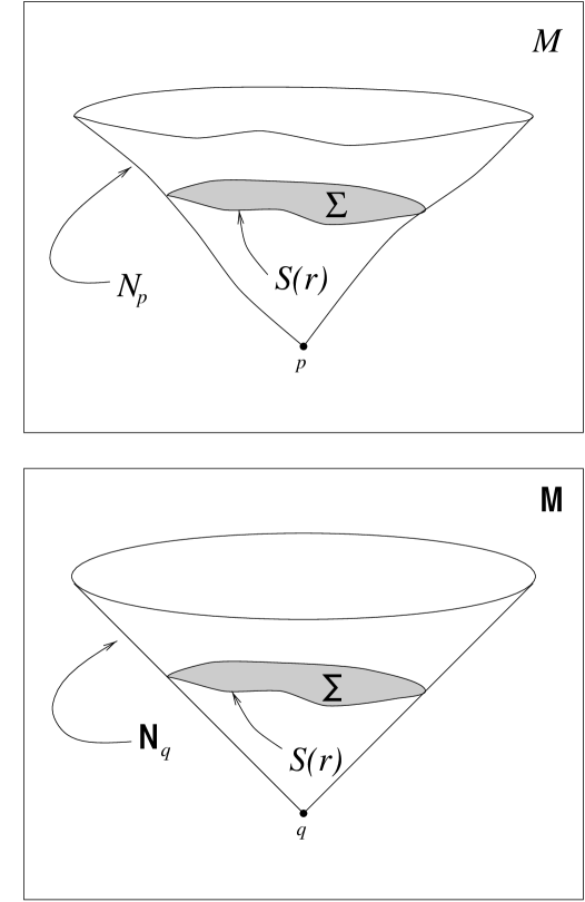
FIG. 1.: Geometry of the Lightcone Reference.

Respectively, the top and bottom boxes depict the physical and reference spacetimes. In the top box the shaded surface spanning $S(r)$ is the 3-surface $\Sigma$, while in the bottom box the shaded surface spanning $S(r)$ is the 3-surface ${\mathsf{\Sigma}}$. Whether viewed as the intersection $N_{p}\bigcap\Sigma$ or the intersection ${\mathsf{N}}_{q}\bigcap{\mathsf{\Sigma}}$, the 2-surface $S(r)$ has the same intrinsic 2-metric. Our limit construction gives us $\Sigma$, but we must choose ${\mathsf{\Sigma}}$; and, moreover, our choice of ${\mathsf{\Sigma}}$ must be determined solely by the intrinsic 2-metric of $S(r)$. Our choice and its physical motivation are described in Subsection 2.A. However, we note here that, whenever $S(r)$ is at all distorted from perfect roundness (as it generally will be), ${\mathsf{\Sigma}}$ is not flat Euclidean 3-space $E^{3}$ (because the intersection of $E^{3}$ with the genuine lightcone ${\mathsf{N}}_{q}$ would be a round sphere). Choosing such a lightcone reference, we assign the zero value of the energy to that (shaded) portion of ${\mathsf{\Sigma}}$ contained within $S(r)$, and compute the energy of (the shaded portion of) $\Sigma$ relative to this zero-point.

REFERENCES

- [1] See, for instance, J. W. York, Found. Phys. 16, 249 (1986).
- [2] J. N. Goldberg, in General Relativity and Gravitation, vol. 1, edited by A. Held (Plenum Press, New York, 1980).
- [3] A. J. Dougan and L. J. Mason, Phys. Rev. Lett. 67, 2119 (1991).
- [4] L. B. Szabados, Class. Quantum Grav. 11, 1833 (1994); Class. Quantum Grav. 11, 1847 (1994); Class. Quantum Grav. 13, 1661 (1996).
- [5] C. Lanzcos, The Variational Principles of Mechanics, (University of Toronto Press, Toronto, 1970).
- [6] J. D. Brown and J. W. York, Phys. Rev. D47, 1407 (1993).
- [7] J. W. York, Phys. Rev. D33, 2092 (1986); J. D. Brown, E. A. Martinez, and J. W. York, Phys. Rev. Lett. 66, 2281 (1991); J. D. Brown and J. W. York, Phys. Rev. D47, 1420 (1993).
- [8] J. D. Brown, S. R. Lau, and J. W. York, Phys. Rev. D55, 1977 (1997).
- [9] J. D. Brown, S. R. Lau, and J. W. York, “Boosted Quasilocal Energy in General Relativity” (manuscript in preparation).
- [10] G. T. Horowitz and B. G. Schmidt, Proc. R. Soc. Lond. A 381, 215 (1982).
- [11] R. M. Kelly, K. P. Tod, and N. M. J. Woodhouse, Class. Quantum Grav. 3, 1151 (1986).
- [12] A. J. Dougan, Class. Quantum Grav. 9, 2461 (1992).
- [13] H. Friedrich, Proc. R. Soc. Lond. A 375, 169 (1981).
- [14] D. Christodoulou and S. Klainerman, The Global Nonlinear Stability of Minkowski Space (Princeton University Press, Princeton, 1993).
- [15] A. Anderson, Y. Choquet-Bruhat, and J. W. York, Topological Methods in Nonlinear Analysis 10, 353 (1997).
- [16] J. W. York, in Gravitation and Geometry, eds. W. Rindler and A. Trautman (Bibliopolis, Naples, 1987).
- [17] T. Newman and K. P. Tod, in General Relativity and Gravitation, vol. 2, edited by A. Held (Plenum Press, New York, 1980).
- [18] R. Penrose and W. Rindler, Spinors and Spacetime, vol. 1, (Cambridge University Press, Cambridge, 1985).
- [19] C. W. Misner, K. S. Thorne, J. A. Wheeler, Gravitation (Freeman, San Francisco, 1973).