Cosmological Pair Production of Charged and Rotating Black Holes

Abstract

We investigate the general process of black hole pair creation in a cosmological background, considering the creation of charged and rotating black holes. We motivate the use of Kerr-Newmann-deSitter solutions to investigate this process, showing how they arise from more general C-metric type solutions that describe a pair of general black holes accelerating away from each other in a cosmological background. All possible KNdS-type spacetimes are classified and we examine whether they may be considered to be in full thermodynamic equilibrium. Instantons that mediate the creation of these space-times are constructed and we see that they are necessarily complex due to regularity requirements. Thus we argue that instantons need not always be real Euclidean solutions to the Einstein equations. Finally, we calculate the actions of these instantons and find that the standard action functional must be modified to correctly take into account the effects of the rotation. The resultant probabilities for the creation of the space-times are found to be real and consistent with the interpretation that the entropy of a charged and rotating black hole is the logarithm of the number of its quantum states.

1 Introduction

A considerable interest in black hole pair production has developed in recent years. Inspired by the well understood particle pair production of quantum field theory (for example $2\gamma\rightarrow e^{+}+e^{-}$), theorists have investigated the possibility that a space-time with a source of excess energy will quantum tunnel into a space-time containing a pair of black holes. The earliest investigations considered pair creation due to background electromagnetic fields [1, 2] but since then have been extended to include pair creation due to cosmological vacuum energy [3, 4] ,cosmic strings [5], and domain walls [6]. These studies have repeatedly provided us with evidence that the exponential of the entropy of a black hole does indeed correspond to the number of its quantum states. However to date they have all concentrated on the creation of non-rotating black holes.

We seek here to extend black hole pair production to include the creation of rotating black holes. As in the extant work we operate within the framework of the path integral formulation of quantum gravity, in which the probability amplitude for the creation of a pair of black holes is approximated by $e^{-I_{i}}$, where $I_{i}$ is the action of a relevant instanton i.e. an imaginary-time solution to the field equations which interpolates between the states before and after the pair of black holes is produced.

To study the pair creation of rotating black holes we proceed in stages. At the first stage, we obtain a solution to the Einstein-Maxwell equations that describes an appropriate pair of black holes accelerating away from each other. Second, we construct an instanton that interpolates between this solution and some appropriate set of initial conditions. Finally, we calculate the action of this instanton, yielding the creation rates for the black hole pairs.

The generalized $C$ metric of [7] describes a pair of black holes with opposite charge and rotation that are uniformly accelerating away from each other in a background with a cosmological constant. As such, it is the sought after solution to the Einstein-Maxwell equations describing the space-times that we wish to create. However, unless the rate of acceleration of the holes is carefully chosen to match that accounted for by the cosmological constant, these solutions will necessarily include cosmic strings or “rods” that provide the pressures/tensions necessary to account for the rest of the acceleration of the holes. Such structures manifest themselves as conical singularities in the metrics. In this paper we will consider pair creation that is driven exclusively by the cosmological vacuum energy and so start out by removing such singularities from the metrics.

Once a suitable class of solutions to the Einstein-Maxwell equations are in hand, we construct instantons to mediate the creation of said space-times. To describe the creation of rotating black holes we find it necessary to consider complex metrics so that the corresponding instantons may be successfully matched to physical solutions. This represents a departure from the usual viewpoint that the instanton actions in the path integral formulation must always be obtained from real, positive-definite (i.e. Euclidean) metrics, obtained by analytically continuing the parameters of the Lorentzian solution to imaginary values. For rotating black holes, this procedure involves supplementing the analytic continuation $t\to it$ with the transformation $J\to iJ$, where $J$ is the real angular momentum [8]. However (as noted previously [9]) such an object has little to do with a physical (Lorentzian) black hole, and we find that this prescription cannot consistently define an instanton that will mediate the pair creation of charged rotating black holes. Despite our usage of complex metrics, the Euclidean action associated with such instantons is always real, and the probabilities are well defined. In particular we find for all allowed instantons that the rate of pair creation is inversely proportional to the exponential of the total entropy of the black hole solutions, consistent with the expectation that black hole entropy is indeed associated with some (as yet unknown) degrees of freedom.

The outline of our paper is as follows. In section two we present a brief review of the path-integral formalism we employ. In section three we start by considering the general class of cosmological charged rotating C-metrics, and show how a consideration of the removal of their conical singularities leads us to the Kerr-Newman-deSitter (KNdS) metrics. As a (useful) preliminary to the pair creation calculations, we then exhaustively classify the possible KNdS space-times. Since pair creation studies usually assume that the created space-times are in a state of thermodynamic equilibrium, we finish section three by considering the KNdS space-times in that light.

In the fourth section we construct instantons that will mediate the creation of these space-times. According to the standard prescription for instanton construction we begin our constructions by analytically continuing the time to imaginary values. For rotating space-times this does not result in a real Euclidean metric, but rather in a complex metric, as noted above. We find that such complex metrics are demanded by the standard Euclidean formalism, and from them construct instantons for each of the space-times considered in section three.

Finally, in section five we calculate actions for these instantons in order to estimate pair creation rates for the space-times of section three. The inclusion of rotation in these calculations is somewhat subtle, and we make use of the quasi-local formalism of Brown and York [10] in order to determine the functional form of the action that should be used to carry out these calculations. We obtain results that are consistent with earlier work on non-rotating black holes: that is, pair creation rates of black holes are always suppressed relative to the creation rate of pure de Sitter space-time and such rates are inversely proportional to the exponential of one quarter of the sum of the areas of their black hole/cosmological horizons. Since the creation rate is inversely proportional to the number of microstates, and since the area is proportional to the entropy of a given black hole space-time, this provides evidence that black hole entropy is indeed given by the logarithm of the number of microstates in the rotating case as well.

2 The Path Integral Formalism

In this section we briefly review the path integral formalism of quantum mechanics as it applies to a relativistic system with both gravitational and electromagnetic fields.

Given a system whose classical evolution is governed by a lagrangian function $L$, a standard problem of quantum mechanics is to calculate the probability that the system passes from an initial state $X_{1}$ to a final state $X_{2}$. In a non-relativistic system each of these states may be described by specifying the state of the entire system at the corresponding instants of time $t_{1}$ and $t_{2}$. Of course for a relativistic system the concept of an instant of time is not so easily defined. For a four dimensional vacuum space-time with gravitational and electromagnetic fields the equivalent concept is to specify a three-manifold $\Sigma$ with Riemannian metric $h_{ij}$, a symmetric tensor field $K_{ij}$ (the extrinsic curvature, that physically describes how the spatial slice is evolving at that “instant of time”), and two vector fields $E^{i}$ and $B^{j}$ that describe the electric and magnetic fields on $\Sigma$. In addition, in vacuo these four fields must satisfy the following constraint equations,

$${\mathcal{H}} \equiv {}^{(3)}R+K^{2}-K^{ij}K_{ij}-2(E^{2}+B^{2})=0$$ (1)

$${\mathcal{H}}_{i} \equiv D_{j}K_{i}^{\;j}-D_{i}K-2\varepsilon_{ijk}E^{j}B^{k}=0$$ (2)

$${\mathcal{F}}_{el} \equiv D_{j}E^{j}=0$$ (3)

$${\mathcal{F}}_{mg} \equiv D_{j}B^{j}=0,$$ (4)

where ${}^{(3)}R$ is the Ricci scalar for $(\Sigma,h)$, $K=h^{ij}K_{ij}$, $E^{2}=h_{ij}E^{i}E^{j}$, $B^{2}=h_{ij}B^{i}B^{j}$, $D_{j}$ is the covariant derivative on $\Sigma$ that is compatible with $h_{ij}$, and $\varepsilon_{ijk}$ is the three dimensional Levi-Cevita tensor. These equations are the Einstein-Maxwell equations projected onto a spatial hypersurface. They ensure that the spatial slice along with its fields may be embedded in a larger four dimensional solution of the Einstein-Maxwell equations (in fact, if $\Sigma$ is a Cauchy surface they uniquely determine that solution via the evolution equations). Geometrically, the extrinsic curvature describes the shape of that embedding.

The path integral approach to quantum mechanics then gives us a prescription for calculating the probability that the system will pass from $X_{1}$ to $X_{2}$. First, we must consider all possible interpolations (or “paths”) between the states (not just those that would be allowed by the classical evolution of the system). This means that we must consider all four-manifolds $M$, metric fields $g_{\alpha\beta}$ and electromagnetic field tensors $F_{\alpha\beta}$ on those manifolds such that the surfaces $\Sigma_{1}$ and $\Sigma_{2}$ and their accompanying fields, may be embedded in $M$ and its accompanying fields . We reiterate that the space-times $(M,g_{\alpha\beta},F_{\alpha\beta})$ are not, in general, solutions to the Einstein-Maxwell equations.

Second, the action

$$I[M_{\Sigma_{2}-\Sigma_{1}},g_{ab},F_{ab}]=\int_{M_{\Sigma_{2}-\Sigma_{1}}}d^{4}x\sqrt{-g}L(g_{ab},F_{ab})+\mbox{ (boundary terms) },$$ (5)

for each path must be calculated, where the integration is over all of $M$ between the two embedded surfaces $\Sigma_{2}$ and $\Sigma_{1}$ and the boundary terms are calculated on the boundaries of $M$ that are consistent with the boundaries of $\Sigma_{1}$ and $\Sigma_{2}$. They will be discussed in more detail later in this section and then in much more detail in section 5.

Third, each of these actions is used to assign a probability amplitude to its associated path. These amplitudes are then summed over all of the possible paths to give a net probability amplitude that the system passes from $X_{1}$ to $X_{2}$. This summation is represented as a functional integral over all of the possible manifold topologies, metrics, and vector potentials $A_{\alpha}$ (generating the field strength $F_{\alpha\beta}$) interpolating between the two surfaces. That is,

$$\Psi_{12}=\int d[M]d[g]d[A]e^{-iI[M,g,F]}\qquad.$$ (6)

Thus in principle, the probability that a space-time initially in a state $(\Sigma,h_{ij},K_{ij},E_{i},B_{i})_{1}$ passes to a state $(\Sigma,h_{ij},K_{ij},E_{i},B_{i})_{2}$ is proportional to $|\Psi_{12}|^{2}$ (we have not normalized the wave function). Unfortunately, as intuitively appealing as this formulation is, the integral (6) cannot be directly calculated. In the first place, there is no known way to define a measure for the integral. Second, even if such a measure were known, it seems quite likely that calculation of the integral would be impractical considering the uncountably infinite number of paths from $X_{1}$ to $X_{2}$.

Fortunately there is a well-motivated simplifying assumption available. In analogy with flat-space calculations, it is argued [11] that to lowest order in $\hbar$, the probability amplitude may be approximated (up to a normalization factor) by

$$\Psi_{12}\approx e^{-I_{c}}$$ (7)

where $I_{c}$ is the real action of a (not necessarily real) Riemannian solution to the Einstein-Maxwell equations that smoothly interpolates between the given initial and final conditions. Essentially, we have assumed that such a solution is a saddle point of the path integral. This solution (if it exists) is referred to as an instanton. The probability that such a tunnelling occurs is then proportional to $|\Psi_{12}|^{2}\approx e^{-2I_{c}}$. Note that this interpretation requires that the action $I_{c}$ be real and positive, and that the fields satisfy the conditions (1–4) so that the instanton smoothly matches onto the Lorentzian solution.

We keep in mind that such Riemannian solutions are typically constructed by analytically continuing the time coordinate $t$ of a Lorentzian solution to $i\tau$, and thereby changing the signature of the metric. As we have already noted, for rotating black holes such a continuation is not sufficient to turn a Lorentzian solution into a real Riemannian one. This issue will be dealt with in some detail in section four.

Note also that it is not necessary for the instanton to have both initial and final conditions. If we can find a smooth Riemannian solution whose only boundary matches the final conditions $X_{2}$, then we can interpret the resultant probability as that for the creation of the 3-space $\Sigma$ from nothing. In that case we have chosen the initial boundary condition to be the no boundary condition of cosmology [12].

As it stands, there is a gap in the above programme. Specifically, we have ignored the fact that the action (5) which generates the classical equations of motion is not unique. Boundary terms consistent with the symmetries of the theory may always be added to the action without affecting the equations of motion. In order to make the right choice of action we must reinterpret the path integral formalism in terms of partition functions and thermodynamics. We will postpone this issue until the computation of the action in section five.

We turn next to a consideration of charged and rotating cosmological C-metrics.

3 Rotating Black Hole Pairs

In this section we examine solutions that describe two black holes accelerating away from each other in a universe with a positive cosmological constant. In the first part, we shall examine the general solution describing such a situation and see how conservation of energy demands that the black hole acceleration rate be matched to the acceleration of the universe as a whole. We shall see that this concern forces us to consider Kerr-Newmann-deSitter (KNdS) space-times as the end states of black hole pair creation processes. As such we will classify the full range of these space-times. Finally, we will consider how quantum effects cause these solutions to evolve in time.

3.1 The Generalized C-metric

The well-known C-metric solution to the Einstein equations (first interpreted in [13]) describes a pair of uncharged and non-rotating black holes that are uniformly accelerating away from each other. In [7] this metric was generalized to allow the holes to be charged and rotating, as well as to allow the inclusion of a cosmological constant and NUT parameter.

In general, space-times of this type contain conical singularities. Physically these arise if the rate of acceleration of the black holes does not match the energy source available to accelerate them. Thus, in the cosmological case, if the black holes are accelerating faster or more slowly than the rest of the universe, conical singularities will exist. Physically, they may be interpreted as cosmic strings or “rods” that are pulling the black holes apart (or pushing them back together) so as to make them accelerate faster (or slower) than the rate of expansion of the universe. If we do not wish to consider such structures, then conservation of energy requires that we match the accelerations of the holes to the source of background energy and thereby eliminate the conical singularities.

Here we demonstrate that one class of conical singularity free solutions of the generalized C-metric are the Kerr-Newmann-deSitter solutions. In other words, the KNdS solution may be viewed as a pair of oppositely charged and rotating black holes accelerating away from each other at a rate that matches the cosmological constant driven rate of acceleration of the universe as a whole. The generalized C-metric takes the form

$$ds^{2}=\frac{1}{(p-q)^{2}}\left[\frac{1+p^{2}q^{2}}{P}dp^{2}+\frac{P}{1+p^{2}q^{2}}\left(d\sigma-q^{2}d\tau\right)^{2}-\frac{1+p^{2}q^{2}}{Q}dq^{2}+\frac{Q}{1+p^{2}q^{2}}\left(p^{2}d\sigma+d\tau\right)^{2}\right],$$ (8)

with accompanying electromagnetic field defined by the vector potential

$$A=-\frac{e_{0}q(d\tau+p^{2}d\sigma)}{1+p^{2}q^{2}}+\frac{g_{0}p(d\sigma-q^{2}d\tau)}{1+p^{2}q^{2}},$$ (9)

where $p,q,\tau$, and $\sigma$ are coordinate functions,

$$P(p)=(-\frac{\Lambda}{6}-g_{0}^{2}+\gamma)+2np-\epsilon p^{2}+2mp^{3}+(-\frac{\Lambda}{6}-e_{0}^{2}-\gamma)p^{4},$$ (10)

and $Q(q)=P(q)+\frac{\Lambda}{3}(1+q^{4})$. $\Lambda$ is the cosmological constant, $\gamma$ and $\epsilon$ are constants connected in a non-trivial way with rotation and acceleration, $e_{0}$ and $g_{0}$ are linear multiples of electric and magnetic charge, and $m$ and $n$ are the respectively mass and the NUT parameter (up to a linear factor). This solution can be analytically extended across the coordinate singularity at $p=q$, so that on the other side of $p=q$ we have a mirror image of the initial solution. Thus, if we view it as describing a pair of black holes, the two holes will be on opposite sides of that $p=q$ hypersurface.

In adaptations of this metric to more specific physical situations, the coordinate functions are associated with the more common spherical-type space-time coordinates as $q\leftrightarrow\frac{1}{r}$, $p\leftrightarrow p_{\alpha}+\alpha\cos\theta$ for some constants $\alpha$ and $p_{\alpha}$, $\sigma\leftrightarrow\phi$ and $\tau\leftrightarrow t$. Now in general, a periodic identification of $\sigma$ will introduce conical singularities at the roots of $P$. To avoid such singularities restrictions must be placed on the constants defining $P$. Defining $p_{\alpha}$, $p_{\beta}$, $\alpha$, and $\beta$ so that the roots of $P(p)$ are at $p_{\alpha}+\alpha$, $p_{\alpha}-\alpha$, $p_{\beta}+i\beta$, and $p_{\beta}-i\beta$, we may write $P$ as

$$P(p)=-C([p-p_{\alpha}]^{2}-\alpha^{2})([p-p_{\beta}]^{2}+\beta^{2}),$$ (11)

where $C=-\frac{\Lambda}{6}-e_{0}^{2}-\gamma$. We begin to specialize by assuming that only $p_{\alpha}-\alpha$ and $p_{\alpha}+\alpha$ are real roots, $p_{\alpha}-\alpha<p_{\alpha}+\alpha$ and $p_{\beta},\beta\in{\mathbb{R}}$. Then there are only two real roots. Restricting $p$ to lie between these two roots, we may reparameterize it as $p=p_{\alpha}+\alpha\cos\theta$, where as usual $\theta\in[0,\pi]$. Then if $p_{\beta}=p_{\alpha}$ (that is, $P(p)$ has an axis of symmetry along the line $p=p_{\alpha}$), potential conical singularities at $p_{\alpha}-\alpha$ or $p_{\alpha}+\alpha$ may be simultaneously eliminated if we identify $\sigma$ with period $T=\frac{4\pi}{P^{\prime}(p_{\alpha}-\alpha)}$ where $P^{\prime}=\frac{dP}{dp}$.

Next, we make the following extended series of coordinate transformations/definitions:

$$q = \frac{1}{\sqrt{\frac{\Lambda}{3}}\beta r},$$ (12)

$$p_{\alpha} = \sqrt{\frac{\Lambda}{3}}\beta\tilde{p_{\alpha}},$$ (13)

$$p_{\beta} = \sqrt{\frac{\Lambda}{3}}\beta\tilde{p_{\beta}},$$ (14)

$$\alpha = \sqrt{\frac{\Lambda}{3}}\beta\tilde{\alpha},$$ (15)

$$\chi^{2} = 1+\frac{\Lambda}{3}\tilde{\alpha}^{2},$$ (16)

$$\sigma = \frac{\phi}{\sqrt{\frac{\Lambda}{3}}C\beta^{3}\tilde{\alpha}\chi^{2}},$$ (17)

$$\tau = \frac{t-\tilde{\alpha}\phi}{\sqrt{\frac{\Lambda}{3}}C\beta\chi^{2}},$$ (18)

$${\mathcal{H}} = 1+\frac{\Lambda}{3}\tilde{\alpha}^{2}\cos^{2}\theta,$$ (19)

$${\mathcal{G}} = r^{2}+(\tilde{p_{\alpha}}+\tilde{\alpha}\cos\theta)^{2},\mbox{ and}$$ (20)

$${\mathcal{Q}}(r) = -\frac{\Lambda}{3C}r^{4}Q(q).$$ (21)

Further, equating (10) and (11) we note the following three equalities relating the two forms of $P$:

$$m = 2Cp_{\alpha}$$ (22)

$$n = Cp_{\alpha}(2p_{\alpha}^{2}-\alpha^{2}+\beta^{2}),\mbox{ and}$$ (23)

$$g_{0}^{2}+e_{0}^{2} = C(1+[p_{\alpha}^{2}-\alpha^{2}][p_{\alpha}^{2}+\beta^{2}])-\frac{\Lambda}{3}.$$ (24)

Then, after a significant amount of algebra, these transformations and equations will modify the metric (8) to become

$$ds^{2}=\frac{\Lambda}{3C(1-\frac{\Lambda}{3}\beta^{2}r[\tilde{p_{\alpha}}+\tilde{\alpha}\cos\theta])^{2}}\left\{\begin{array}[]{lll}\frac{{\mathcal{G}}}{{\mathcal{H}}}d\theta^{2}&+&\frac{{\mathcal{H}}\sin^{2}\theta}{{\mathcal{G}}\chi^{4}}\left(\tilde{\alpha}dt+[r^{2}+\tilde{\alpha}^{2}]d\phi\right)^{2}\\ +\frac{{\mathcal{G}}}{{\mathcal{Q}}}dr^{2}&-&\frac{{\mathcal{Q}}}{{\mathcal{G}}\chi^{4}}\left(dt+\left[(\frac{\tilde{p_{\alpha}}^{2}}{\tilde{\alpha}}+2\tilde{p_{\alpha}}\cos\theta)-\tilde{\alpha}\sin^{2}\theta\right]d\phi\right)^{2}\end{array}\right\}.$$ (25)

Setting $e_{0}=\sqrt{\frac{\Lambda}{3}}E_{0}\beta^{2}$, $g_{0}=\sqrt{\frac{\Lambda}{3}}G_{0}\beta^{2}$, and $\tilde{p_{\alpha}}=M\beta^{2}$, we may write ${\mathcal{Q}}$ as,

$${\mathcal{Q}}(r) = -\frac{\Lambda}{3}\left(\frac{1-(E_{0}^{2}+G_{0}^{2})(M^{2}\beta^{4}-\tilde{\alpha}^{2})(1+\frac{\Lambda}{3}M^{2}\beta^{4})\beta^{8}}{1-(E_{0}^{2}+G_{0}^{2})\beta^{4}}\right)r^{4}$$ (26)

$$-2\frac{\Lambda}{3}M\left(1+\frac{\Lambda}{3}(2M^{2}\beta^{4}-\tilde{\alpha}^{2})\right)\beta^{2}r^{3}+(1+\frac{\Lambda}{3}(6M^{2}\beta^{4}-\alpha^{2}))r^{2}$$

$$-2Mr+\frac{E_{0}^{2}+G_{0}^{2}+(\tilde{\alpha}^{2}-M^{2}\beta^{4})(1+\frac{\Lambda}{3}M^{2}\beta^{4})}{1+(E_{0}^{2}+G_{0}^{2})\beta^{4}}.$$

The $r^{3}$ term of the above is identified with the NUT parameter. If we wish to set this equal to zero but keep the mass parameter $M$ non-zero, then we must set one of $\beta$ or $1+\frac{\Lambda}{3}(M^{2}\beta^{4}-\tilde{\alpha}^{2})$ to zero. Here we choose to take the limit as $\beta\rightarrow 0$ (choosing $1+\frac{\Lambda}{3}(M^{2}\beta^{4}-\tilde{\alpha}^{2})=0$ results in a metric that is similar to but not quite the KNdS metric - most notably it retains the leading conformal factor). Then, if we replace $\tilde{\alpha}$ with the more traditional symbol $a$ the metric becomes the standard Kerr-Newmann-deSitter metric (and similarly the vector potential $A$ becomes a vector potential that generates the associated electromagnetic field) which will be discussed in some detail in the rest of this section. Thus, the KNdS metric describes two black holes in deSitter space that are accelerating away from each other due to the cosmological expansion of the universe.

Before continuing, we pause to comment that there are other ways to eliminate the conical singularities in (8). Although most yield the KNDS metric, some will give rise to other space-times. These will not be considered in the present paper.

3.2 The Basic Kerr-Newmann-deSitter Solution

In Boyer-Lindquist type coordinates, the Kerr-Newmann-deSitter metric takes the form [14]

$$ds^{2}=-\frac{{\mathcal{Q}}}{{\mathcal{G}}\chi^{4}}\left(dt-a\sin^{2}\theta d\phi\right)^{2}+\frac{{\mathcal{G}}}{{\mathcal{Q}}}dr^{2}+\frac{{\mathcal{G}}}{{\mathcal{H}}}d\theta^{2}+\frac{{\mathcal{H}}\sin^{2}\theta}{{\mathcal{G}}\chi^{4}}\left(adt-\left[r^{2}+a^{2}\right]d\phi\right)^{2},$$ (27)

where

$${\mathcal{G}}\equiv r^{2}+a^{2}\cos^{2}\theta,\;\;\;{\mathcal{H}}=1+\frac{\Lambda}{3}a^{2}\cos^{2}\theta,\;\;\;\chi^{2}=1+\frac{\Lambda}{3}a^{2},\mbox{ and}$$ (28)

$${\mathcal{Q}}=-\frac{\Lambda}{3}r^{4}+\left(1-\frac{\Lambda}{3}a^{2}\right)r^{2}-2Mr+\left(a^{2}+E_{0}^{2}+G_{0}^{2}\right).$$

The individual solutions are defined by the values of the parameters $\Lambda$, $a$, $M$, $E_{0}$, and $G_{0}$ which are respectively the cosmological constant (since we are interested in deSitter type space-times, we will assume that it is positive), the rotation parameter, the mass, and the effective electric and magnetic charge of the solution. Along with the electromagnetic field

$$F=-\frac{1}{{\mathcal{G}}^{2}\chi^{2}}\left\{Xdr\wedge(dt-a\sin^{2}\theta d\phi)+Y\sin\theta d\theta\wedge(adt-(r^{2}+a^{2})d\phi)\right\},$$ (29)

where $X=E_{0}\Gamma+2aG_{0}r\cos\theta$, $Y=G_{0}\Gamma-2aE_{0}r\cos\theta$, and $\Gamma=r^{2}-a^{2}\cos^{2}\theta$, this metric is a solution to the Einstein-Maxwell equations. For future reference we note that a vector potential generating this field is

$$A=\frac{E_{0}r}{{\mathcal{G}}\chi^{2}}\left(dt-a\sin^{2}\theta d\phi\right)+\frac{G_{0}\cos\theta}{{\mathcal{G}}\chi^{2}}\left(adt-\left(r^{2}+a^{2}\right)d\phi\right).$$ (30)

The roots of the polynomial ${\mathcal{Q}}$ correspond to horizons of the metric. As a quartic with real coefficients, ${\mathcal{Q}}$ may have zero, two, or four real roots. We are interested in black hole space-times, and so shall assume that there are four real roots, and that three of them are positive. In ascending order the horizons corresponding to the positive roots are the inner and outer black hole horizons, and the cosmological horizon.

Let the roots of ${\mathcal{Q}}$ in increasing order be $d-\delta$, $d+\delta$, $e-\varepsilon$, and $e+\varepsilon$, where $e$ and $d$ are reals and $\varepsilon$ and $\delta$ are non-negative reals. The absence of a cubic term in ${\mathcal{Q}}$ forces $d=-e$. Two further restrictions:

$$\begin{array}[]{ccccl}0&\leq&\varepsilon&<&e,\mbox{ and}\\ e&<&\delta&\leq&2e-\varepsilon\end{array}$$

ensure that the roots are ordered as we have proposed. Then we may write ${\mathcal{Q}}$ without loss of generality as

$${\mathcal{Q}}=-\frac{\Lambda}{3}\left((r-e)^{2}-\varepsilon^{2}\right)\left((r+e)^{2}-\delta^{2}\right).$$ (31)

If all of the roots of ${\mathcal{Q}}$ are distinct (we shall deal with the degenerate cases in subsections 3.4, 3.5, and 3.6), then by the standard Kruskal techniques the metric may be analytically continued through the horizons to obtain the maximal extension of the space-time [15]. Though this maximal extension is infinite in extent, a variety of other global structures are possible if we choose to make periodic identifications within it. In particular, if we demand that there be no closed time-like curves in the space-time and also wish to have two black holes in $t=\mbox{constant}$ spatial cross-sections, then the global structure is uniquely determined and is shown in figure 1 (for a two dimensional $\phi=\mbox{constant}$, $\theta=\frac{\pi}{2}$ cross section). The $t=\mbox{constant}$ spatial hypersurfaces are closed and each span the two black hole regions, cutting through the intersections of both the $r=r_{c}$ and $r=r_{o}$ lines. The matching conditions are such that, in the spatial hypersurfaces, the two holes have opposite spins as well as opposite charges. Thus, the net charge and net spin of the system are both zero. We note that it is not possible to periodically identify the space-time such that the spatial sections contain only a single black hole.

Figure 1: The global structure for the KNdS solutions - with periodic identifications to ensure that $t=\mbox{constant}$ hypersurfaces contain only two black holes. As indicated the figure is repeated vertically and periodically identified horizontally. $r=r_{c}$ is the cosmological horizon, $r=r_{o}$ is the outer black hole horizon, and $r=r_{i}$ is the inner black hole horizon. The wavy lines at $r=0$ represent the ring singularity found there for $a\neq 0$. If $a=0$ then this singularity may not be avoided and the space-time cuts off at $r=0$. Otherwise the singularity may be bypassed and we may proceed to negative values of $r$. $r=r_{-}$ is the (negative) fourth root of ${\mathcal{Q}}$.

Next, we consider the range of the parameters for which our conditions on the roots of ${\mathcal{Q}}$ will hold.

3.3 The Allowed Range of the KNdS Solutions

The requirement that ${\mathcal{Q}}$ has three positive real roots enforces restrictions on the allowed values of the physical parameters $a$, $M$, $E_{0}$, and $G_{0}$. ${\mathcal{Q}}$ is a quartic, and so in principal we may solve it exactly and decide under what circumstances it has four real roots. In practice however, the exact solution to a quartic is too messy to work with. Thus, we tackle the problem in reverse. We will first determine the allowed ranges of the ${\mathcal{Q}}$ structure parameters $e$, $\delta$, and $\varepsilon$, and then use these to parameterize the allowed range of the physically meaningful parameters $a$, $M$, $E_{0}$, and $G_{0}$.

Matching (3.2) with (31) we obtain expressions for the physical parameters in terms of the structure parameters:

$$a^{2} = \frac{3}{\Lambda}-\delta^{2}-\varepsilon^{2}-2e^{2},$$ (32)

$$M = \frac{\Lambda}{3}(\delta^{2}-\varepsilon^{2})e,\mbox{ and}$$ (33)

$$E_{0}^{2}+G_{0}^{2} = \frac{\Lambda}{3}(\delta^{2}-e^{2})(e^{2}-\varepsilon^{2})+(\delta^{2}+\varepsilon^{2}+2e^{2})-\frac{3}{\Lambda}.$$ (34)

Requiring that each of these parameters be non-negative will impose further restrictions (beyond the root ordering conditions (3.2)) on the allowed ranges of $e$, $\varepsilon$, and $\delta$. Requiring that $a^{2}\geq 0$ we obtain the condition

$$\frac{3}{\Lambda}-\delta^{2}-\varepsilon^{2}-2e^{2}\geq 0.$$ (35)

$M$ will automatically be non-negative because of the root-ordering conditions (3.2) while requiring that $E_{0}^{2}+G_{0}^{2}\geq 0$ we obtain

$$\frac{\Lambda}{3}(\delta^{2}-e^{2})(e^{2}-\varepsilon^{2})+(\delta^{2}+\varepsilon^{2}+2e^{2})-\frac{3}{\Lambda}\geq 0.$$ (36)

In order to disentangle these structure parameters we rescale them as follows. $\Lambda$ and $e$ are non-zero so we may define $\Delta$, $E$, and $X$ by:

$$\delta\equiv\Delta e,\mbox{ }\varepsilon\equiv Ee,\mbox{ and }e\equiv\sqrt{\frac{3}{\Lambda}}X.$$ (37)

Then, the conditions (35) and (36) become respectively,

$$1-(\Delta^{2}+E^{2}+2)X^{2}\geq 0,\mbox{ and }$$ (38)

$$(\Delta^{2}-1)(1-E^{2})X^{4}+(\Delta^{2}+E^{2}+2)X^{2}-1\geq 0$$ (39)

The first of these provides an upper bound on the allowed range $X$ for given values of $\Delta$ and $E$. $a^{2}\geq 0$ if and only if

$$X\leq X_{U}\equiv\frac{1}{\sqrt{2+\Delta^{2}+E^{2}}}.$$ (40)

In the meantime, (39) is quadratic in $X^{2}$ and so may be easily solved. It turns out that over the allowed ranges of $\Delta$ and $E$, it has only one positive real root. Further, it is upward opening, and therefore the positive real root provides a lower bound for the allowed values of $X$. $E_{0}^{2}+G_{0}^{2}\geq 0$ is and only if

$$X\geq X_{L}\equiv\sqrt{\frac{-(\Delta^{2}+E^{2}+2)+\sqrt{8(E^{2}+\Delta^{2})+(E^{2}-\Delta^{2})^{2}}}{2(\Delta^{2}-1)(1-E^{2})}}.$$ (41)

On plotting $X_{U}$ and $X_{L}$ we find that for $0\leq E\leq 1$ and $1\leq\Delta\leq 2$, $X_{L}\leq X_{U}$ and so there exists a non-zero range for $X$ for all the possible values of $E$ and $\Delta$. With this range of allowed values for $X$ in hand, we now have a parameterization for all the possible KNdS black hole solutions. The parameterization is given by the restrictions

$$1<\Delta\leq 2,\mbox{ }0\leq E<2-\Delta,\mbox{ and }X_{L}\leq X\leq X_{U},$$ (42)

the definitions (37), and the expressions (32)-(34).

These ranges are shown in figure 2. In that figure the allowed parameter range of KNdS space-times is the region bounded by the five sheets defined by $a=0$, $M=0$, $E_{0}^{2}+G_{0}^{2}=0$, $E=0$, and $E=2-\Delta$. The last two conditions are respectively cold black hole space-time where the inner and outer black hole horizons coincide and a Nariai-type space time where the outer black hole horizon coincides with the cosmological horizon (we shall soon see that this apparent degeneracy of the metric is an artifact of the coordinate system and that the distance between the two horizons remains finite and non-zero throughout the limiting process). The intersection of the Nariai and cold sheets is referred to as the ultracold solution. This nomenclature is taken from the corresponding non-rotating instantons discussed in [3], and will be used throughout this work. A special case of solutions labelled the lukewarm solutions is also shown in the figures. It will be discussed in subsections 3.7 and 3.8.

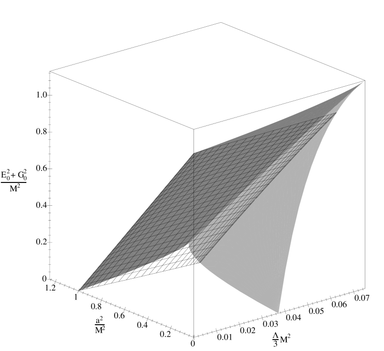
Figure 2: The allowed range of the KNdS parameters. The range is bounded by the planes $M=0$, $a^{2}=0$, $E_{0}^{2}+G_{0}^{2}=0$, the cold solutions (the darkest sheet) and the rotating Nariai solutions (the lighter gray sheet). Also shown as a meshed sheet are the lukewarm solutions.

We have now established the range of KNdS solutions allowed by the structure of the polynomial ${\mathcal{Q}}$. It remains to be demonstrated that the full range is realizable as a set of well defined metrics. In particular the current coordinate representation of the metric breaks down in the Nariai ($\varepsilon\rightarrow 0$, $\delta\neq 0$) and ultracold ($\varepsilon\rightarrow 0$, $\delta\rightarrow 2e-\varepsilon$) cases. In the following three subsections we shall consider how these various limits may be achieved, and we will further consider how the limiting processes affect the global structure of the space-times. We begin with the cold limit ($\delta=2e-\varepsilon$, $\varepsilon\neq 0$).

3.4 The Cold Limit

This limit may be taken without having to make any changes to the coordinate system. Therefore, the metric keeps the form (27) and the electromagnetic field and potential remain as (29) and (30) respectively. The physical parameters are given by:

$$a^{2} = \frac{3}{\Lambda}-2(3e^{2}-2\varepsilon e+\varepsilon^{2})$$ (43)

$$M = \frac{4\Lambda}{3}e^{2}(e-\varepsilon),\mbox{ and}$$ (44)

$$E_{0}^{2}+G_{0}^{2} = \frac{\Lambda}{3}(3e-\varepsilon)(e-\varepsilon)^{2}(e+\varepsilon)+2(3e^{2}-2e\varepsilon+\varepsilon^{2})-\frac{3}{\Lambda},$$ (45)

where the range of the parameters is limited by the relations

$$0< E <1,\mbox{ and}$$ (46)

$$\sqrt{\frac{-3+2E-E^{2}+2\sqrt{3-4E+2E^{2}}}{(3-E)(1+E)(1-E)^{2}}}\leq X \leq\frac{1}{\sqrt{2(E^{2}-2E+3)}}.$$ (47)

As before, $e=\sqrt{\frac{3}{\Lambda}}X$, and $\varepsilon=Ee$.

In this space-time, the double horizon of the black hole recedes to an infinite proper distance from all other parts of the space-time. Thus, the global structure of the space-time changes - in particular, the region inside the black hole is cut off from the rest of the space-time. Again we choose the global structure so that the space-time contains two (in this case extreme) black holes. This structure is shown in figure 3. Note that in this case, the $t=\mbox{constant}$ hypersurfaces consist of two extreme black holes, and so are not closed as they were in the lukewarm case (the horizons recede to infinite proper distance from all other points in the space-time).

Finally, we note for the cases where $a=0$, this solution reduces to the cold solutions discussed in [3].

Figure 3: The Penrose diagram for a two hole cold KNdS space-time. Opposite sides of the rectangle are identified. $r=r_{c}$ is the cosmological horizon and $r=r_{o,i}$ is the double black hole horizon. If $a=0$, then the space-time cuts off at the singularity at $r=0$. Otherwise, we may pass through the ring singularity to the negative values of $r$, including $r_{-}$, the fourth root of ${\mathcal{Q}}$.

3.5 The Nariai Limit

The current coordinate system breaks down in the $\varepsilon=0$ limit. Specifically, for $\varepsilon=0$, $r=e$ (becomes a constant), and ${\mathcal{Q}}=0$, so the coordinate system becomes degenerate, and the metric ill-defined. These problems may easily be avoided however, if we make the transformations:

$$r = e+\varepsilon\rho.$$ (48)

$$\phi = \varphi+\frac{a}{e^{2}+a^{2}}t,\mbox{ and}$$ (49)

$$t = \frac{(e^{2}+a^{2})\chi^{2}}{\varepsilon}\tau.$$ (50)

Then, the $\varepsilon\rightarrow 0$ limit may be taken without hindrance, and the metric becomes

$$ds^{2}=-{\tilde{{\mathcal{Q}}}}{\mathcal{G}}d\tau^{2}+\frac{{\mathcal{G}}}{{\tilde{{\mathcal{Q}}}}}d\rho^{2}+\frac{{\mathcal{G}}}{{\mathcal{H}}}d\theta^{2}+\frac{{\mathcal{H}}\sin^{2}\theta}{{\mathcal{G}}}\left(2ae\rho d\tau+\frac{e^{2}+a^{2}}{\chi^{2}}d\varphi\right)^{2},$$ (51)

while the electromagnetic field becomes,

$$F=\frac{-X}{{\mathcal{G}}}d\rho\wedge d\tau+\frac{Y\sin\theta}{{\mathcal{G}}^{2}}d\theta\wedge\left(2ae\rho d\tau+\frac{e^{2}+a^{2}}{\chi^{2}}d\varphi\right).$$ (52)

A electromagnetic potential generating this is

$$A=-E_{0}\frac{(e^{2}-a^{2})}{e^{2}+a^{2}}\rho d\tau-\frac{aE_{0}e\sin^{2}\theta+G_{0}(e^{2}+a^{2})\cos\theta}{{\mathcal{G}}(e^{2}+a^{2})}\left(2ae\rho d\tau+\frac{e^{2}+a^{2}}{\chi^{2}}d\varphi\right).$$ (53)

In the above, ${\tilde{{\mathcal{Q}}}}=\frac{\Lambda}{3}(2e-\delta)(1-\rho^{2})(2e+\delta)$, ${\mathcal{G}}=e^{2}+a^{2}\cos^{2}\theta$, $\Gamma=e^{2}-a^{2}\cos^{2}\theta$, $X=E_{0}\Gamma+2aG_{0}e\cos\theta$, and $Y=G_{0}\Gamma-2aE_{0}e\cos\theta$. Note that the above potential is not the simply (30) under the coordinate transformation as the $A$ generated in that way diverges when $\varepsilon\rightarrow 0$. The divergence is removed (and the above result obtained) if we make the gauge transformation $A\rightarrow A-\frac{E_{0}e}{\varepsilon}d\tau$ before we take the coordinate transformation and limit.

The physical parameters are given in terms of $e$ and $\delta$ as:

$$a^{2} = \frac{3}{\Lambda}-2e^{2}-\delta^{2},$$ (54)

$$M = \frac{\Lambda}{3}\delta^{2}e,\mbox{ and}$$ (55)

$$E_{0}^{2}+G_{0}^{2} = \frac{\Lambda}{3}(\delta^{2}-e^{2})e^{2}+(2e^{2}+\delta^{2})-\frac{3}{\Lambda},$$ (56)

and the allowed ranges of $e=\sqrt{\frac{3}{\Lambda}}X$ and $\delta=\Delta e$ are given by

$$1< \Delta \leq 2\mbox{ and}$$ (57)

$$\sqrt{\frac{-(\Delta^{2}+2)+\Delta\sqrt{\Delta^{2}+8}}{2(\Delta^{2}-1)}}\leq X \leq\frac{1}{\sqrt{2+\Delta^{2}}}.$$ (58)

We note that the Nariai solution is no longer a black hole solution. Extending the metric through the horizons by the standard Kruskal techniques, we obtain the Penrose diagram of figure 4 for the ($\tau$,$\rho$) sector. Note that there is no longer a singularity at finite distance beyond either of the horizons, and so this is no longer a black hole space-time. In fact, the diagram is the same as that for two dimensional deSitter space. If there were no rotation ($a=0$), then this space-time would just be the direct product of two dimensional deSitter space, and a two sphere of fixed radius. With rotation, of course the situation is not so simple.

Figure 4: The Penrose diagram for the Nariai limit space-time. $\rho=\pm 1$ are the two cosmological horizons.

If $a=0$, and we make the coordinate transformation $\rho=\cos\chi$, then this solution reduces to the non-rotating charged Nariai solution considered in [3].

Even though the Nariai solution is not a black hole solution itself, it was shown in [16] that an uncharged, non-rotating Nariai solution is unstable with respect to quantum tunnelling into an almost- Nariai Schwarzschild-deSitter space-time. It is usually argued [17] that this tunnelling carries over analogously with the inclusion of charge and rotation - in which case Nariai solutions decay into near Nariai KNdS space-times. Thus, in the future sections of this paper where we study black hole pair creation this solution will remain of interest. Then, a route to black hole pair creation will be to create a Nariai space-time and then let it decay into a black hole pair.

3.6 The Ultracold Limits

Finally we consider the ultracold limits where both $\varepsilon\rightarrow 0$ and $\delta\rightarrow 2e-\varepsilon$. It turns out that there are two such limits which we shall label the ultracold I and II limits. In this subsection we shall only demonstrate how they may be reached from the Nariai limit. Similar coordinate transformations (which sometimes must be iterated two or three times) allow us to reach the same two limits both from the cold limit, and, taking $\delta\rightarrow 2e-\varepsilon$ and $\varepsilon\rightarrow 0$ simultaneously, straight from the non-extreme standard KNdS form of the metric. We deal with the two cases separately.

Ultracold I: Making the transformations,

$$\rho = \eta-\eta k(2e-\delta)R,$$ (59)

$$\varphi = \Phi-2\eta\frac{ae\chi^{2}\tau}{e^{2}+a^{2}},\mbox{ and}$$ (60)

$$\tau = \frac{\eta T}{k(2e-\delta)},$$ (61)

where $\eta=\pm 1$, and $k=8\frac{\Lambda}{3}e$, and taking the limit as $\delta\rightarrow 2e$ we obtain,

$$ds^{2}=-{\mathcal{G}}RdT^{2}+\frac{{\mathcal{G}}}{R}dR^{2}+\frac{{\mathcal{G}}}{{\mathcal{H}}}d\theta^{2}+\frac{{\mathcal{H}}}{{\mathcal{G}}}\sin^{2}\theta\left(2aeRdT+\frac{e^{2}+a^{2}}{\chi^{2}}d\Phi\right)^{2}.$$ (62)

The electromagnetic field and potential become,

$$F=\frac{-X}{{\mathcal{G}}}dR\wedge dT+\frac{Y\sin\theta}{{\mathcal{G}}^{2}}d\theta\wedge\left(2aeRdT+\frac{e^{2}+a^{2}}{\chi^{2}}d\Phi\right),$$ (63)

and,

$$A=-E_{0}\frac{e^{2}-a^{2}}{e^{2}+a^{2}}RdT-\frac{aE_{0}e\sin^{2}\theta+G_{0}(e^{2}+a^{2})\cos\theta}{{\mathcal{G}}(e^{2}+a^{2})}\left(2aeRdT+\frac{e^{2}+a^{2}}{\chi^{2}}d\Phi\right).$$ (64)

$R\in(0,\infty)$, $T\in(-\infty,\infty)$, $\theta\in[0,\pi]$, and $\Phi$ inherits a $2\pi$ periodicity from its predecessors. ${\mathcal{G}}$, ${\mathcal{H}}$, $\chi^{2}$, $X$, and $Y$ all retain their old definitions. Note that the EM potential and field have retained their Nariai form.

The ($R$,$T$) sector of the space-time is conformally the same as the Rindler space-time (which of course is actually a sector of two dimensional Minkowski space). The Rindler horizon is at $R=0$ and as this is the only horizon, the space does not contain black holes. Before giving the parameterization of this solution, we consider the transformations leading to the ultracold II case.

Ultracold II: Making the transformations,

$$\rho = b+k\sqrt{2e-\delta}R,$$ (65)

$$\varphi = \Phi-2\frac{aeb\chi^{2}\tau}{e^{2}+a^{2}},\mbox{ and}$$ (66)

$$\tau = \frac{T}{k\sqrt{2e-\delta}},$$ (67)

where $b\neq\pm 1$, and $k=2\sqrt{\frac{\Lambda}{3}(1-b^{2})e}$ and taking the limit as $\delta\rightarrow 2e$, we obtain,

$$ds^{2}=-{\mathcal{G}}dT^{2}+{\mathcal{G}}dR^{2}+\frac{{\mathcal{G}}}{{\mathcal{H}}}d\theta^{2}+\frac{{\mathcal{H}}}{{\mathcal{G}}}\sin^{2}\theta\left(2aeRdT+\frac{e^{2}+a^{2}}{\chi^{2}}d\Phi\right)^{2}.$$ (68)

The electromagnetic field and potential again take the forms (63) and (64). $R,T\in(-\infty,\infty)$, $\theta\in[0,\pi]$, and $\Phi$ inherits a period of $2\pi$ from its predecessors. ${\mathcal{G}}$, ${\mathcal{H}}$, $X$, and $Y$ again retain their meanings from the Nariai case.

Clearly the ($R$,$T$) sector of this space-time is conformally the same as two dimensional Minkowski flat space. There is no horizon structure, and therefore no black holes.

The physical parameters in both of these cases are given by

$$a^{2} = \frac{3}{\Lambda}-6e^{2},$$ (69)

$$M = 4\frac{\Lambda}{3}e^{3},\mbox{ and}$$ (70)

$$E_{0}^{2}+G_{0}^{2} = \Lambda e^{4}+6e^{2}-\frac{3}{\Lambda},$$ (71)

and the allowed range of $e=\sqrt{\frac{3}{\Lambda}}X$ is given by,

$$\sqrt{-1+\frac{2}{\sqrt{3}}}\leq X \leq\frac{1}{\sqrt{6}}.$$ (72)

Once more we note that when $a=0$ these ultracold cases reduce to the two non-rotating ultra-cold solutions considered in [3]. As noted above, neither of these space-times contains black holes. Still for completeness, we shall continue to include them in our considerations for the rest of the paper.

3.7 Issues of Equilibrium

Before passing on to the next section where we will construct instantons to create the above space-times, we pause to examine whether these solutions to the Einstein-Maxwell equations are stable with respect to semi-classical effects. To this end, we must consider thermodynamically driven particle exchange between the horizons, electromagnetic discharge of the holes (due to emission of charged particles), and spin-down of the holes (due to emission of spinning particles and super-radiance).

It is well known that a black hole emits particles in a black body thermal spectrum and thus may be viewed as having a definite temperature [18]. In the same way, it has been shown that deSitter horizons may also be viewed as black bodies and have a definite temperature [15]. For a space-time with non-degenerate horizons, these temperatures may be most easily calculated by the conical singularity procedure [11] (which we will return to when we construct instantons in the following sections). First, corotate the coordinate system with the horizon for which we are calculating the temperature. Second, analytically continue the time coordinate to imaginary values. For definiteness we will label the imaginary time coordinate ${\mathcal{T}}$, the radial coordinate ${\mathcal{R}}$, and let the horizon be located at ${\mathcal{R}}={\mathcal{R}}_{h}$. Next, consider a curve in the ${\mathcal{T}}-{\mathcal{R}}$ plane with constant radial coordinate ${\mathcal{R}}={\mathcal{R}}_{0}$. Periodically identify the imaginary time coordinate with some period $P_{0}$ so that this curve becomes a coordinate “circle” and may be assigned a radius $R_{0}$ and circumference $C_{0}$ according to the integrals

$$R_{0}\equiv\left.\left(\int_{{\mathcal{R}}_{h}}^{{\mathcal{R}}_{0}}\sqrt{g_{{\mathcal{R}}{\mathcal{R}}}}d{\mathcal{R}}\right)\right|_{{\mathcal{T}}=0},\;\;\;\;\;\mbox{and}\;\;\;\;\;C_{0}\equiv\left.\left(\int_{0}^{P_{0}}\sqrt{g_{{\mathcal{T}}{\mathcal{T}}}}d{\mathcal{T}}\right)\right|_{{\mathcal{R}}={\mathcal{R}}_{0}}.$$ (73)

Finally, calculate $\lim_{{\mathcal{R}}_{0}\rightarrow{\mathcal{R}}_{h}}\frac{C_{0}}{R_{0}}$. Pick the value of $P_{0}$ so that the limit has value $2\pi$. Then, the horizon has temperature $T_{h}=1/P_{0}$, and surface gravity $\kappa_{h}=2\pi/P_{0}$.

If there is a degenerate horizon, as is the case for a cold black hole, then that horizon is an infinite proper distance from all non-horizon points of the space-time. In such a situation there is no restriction on the period with which we may periodically identify the degenerate horizon, and it has been argued [2] that the black hole can therefore be in equilibrium with thermal radiation of any temperature.

We now consider which of our space-times are in thermodynamic equilibrium. First, consider the general, non-extreme KNdS solutions. The temperature of the outer black hole horizon and the cosmological horizon are respectively,

$$T_{bh}=\left.\left(\frac{1}{4\pi\chi^{2}(r^{2}+a^{2})}\frac{d{\mathcal{Q}}}{dr}\right)\right|_{r=r_{bh}}\;\;\;\mbox{and}\;\;\;T_{ch}=\left.\left(\frac{-1}{4\pi\chi^{2}(r^{2}+a^{2})}\frac{d{\mathcal{Q}}}{dr}\right)\right|_{r=r_{ch}}$$ (74)

These two temperatures are equal if and only if, $4\frac{\Lambda}{3}\varepsilon^{2}e(2e^{2}-2a^{2}-\varepsilon^{2}-\delta^{2})=0$. $\varepsilon=0$ corresponds to the Nariai solutions which we will consider momentarily. $e=0$ is disallowed by the root ordering conditions (3.2). This leaves us with $2e^{2}-2a^{2}-\varepsilon^{2}-\delta^{2}=0$ as the only case in which the non- extreme solutions achieve thermodynamic equilibrium. We label this the lukewarm case, in accordance with the instanton labeling scheme of [3]. We will consider the parameterization of these solutions in the next subsection.

The cold limit is in thermodynamic equilibrium at the temperature of the cosmological horizon, for as we have noted an extreme black hole may be in equilibrium with thermal radiation of any temperature. The Nariai limit too is in thermodynamic equilibrium. Both the horizons have the same temperature,

$$T_{Nar}=\frac{\frac{\Lambda}{3}(4e^{2}-\delta^{2})}{4\pi}.$$ (75)

The first ultracold case has only one horizon with temperature

$$T_{UCI}=\frac{1}{2\pi},$$ (76)

and so with no other horizon to balance this one off, it is not in thermal equilibrium. The second ultracold case has no horizons, and so is trivially in equilibrium.

Next we consider discharge of the black holes. Even if the black hole and cosmological horizon are in equilibrium with respect to net particle exchange between them, there will be a net exchange of charge between the horizons. The mechanism is that even though the net numbers (and masses) of created particles may be the same, an excess of charged particles will be created at the black hole horizon, and so it will discharge [19]. This effect may be completely avoided if there are no particles of the appropriate charge that are also lighter than the black hole. Thus, if magnetic monopoles do not exist then the magnetic holes will be stable with respect to discharge. Further, even if the appropriate light charged particles exist, the discharge effects will be small if the temperature of the black hole is small relative to the mass of those particles.

Finally we consider the spin down of the black holes. If the black hole and cosmological horizons are at the same temperature, then there will be no net energy exchange between the horizons, but the particles created at the black hole horizon may still have an excess of angular momentum relative to those created at the cosmological horizon. This effect will tend to be small by itself, but it may be amplified by super-radiance. At this point things become somewhat complicated. Fairly extensive investigations have been conducted into super-radiance effects in the asymptotically flat case [20, 21, 22], but only preliminary results are available for the asymptotically deSitter case [23]. In particular, in [23] only one specific class of non-extreme holes have been studied, and that class is not in thermodynamic equilibrium with the cosmological horizon.

With these caveats in mind, consider the following. The original work by Page [20, 21] showed that for a wide class of massive and massless bosonic and fermionic fields (including the set of fields that we assume to exist in our universe), a spinning black hole (in an asymptotically flat universe) will radiate all of its angular momentum well before it has radiated all of its mass. He also speculated however, that given a large enough number of massless scalar fields, then the ratio of angular momentum to mass would approach a finite value rather than zero. Chambers, Hiscock, and Taylor showed that this in fact would be the case if 32 massless scalar fields exist [22]. Maeda and Tachiwaza [23] showed that a class of uncharged near-extremally rotating black holes in an asymptotically de Sitter space will spin down faster than their counterparts in asymptotically flat space-time. As noted before these holes were not in equilibrium with the cosmological horizon.

Thus, within limits of current knowledge, it is consistent that the rotating holes will spin down to static black holes within finite time. What is not clear however is what the time scale for these effects is (particularly in the case where the horizons are in equilibrium). Further, the extant papers all agree with the physically intuitive idea that if the angular momentum is very small relative to the mass, then the rate of discharge of the holes will be small. These issues will be quantitatively investigated in a future paper. For the remainder of this paper we shall consider only those situations for which discharge and spin-down effects may be neglected.

3.8 The Lukewarm Solution

As discussed in the previous subsection, the lukewarm solution is characterized by $2e^{2}-2a^{2}-\varepsilon^{2}-\delta^{2}=0$. We can use this relation to eliminate $\delta$ from the parameterizations of the physical parameters. We then have:

$$a^{2} = 4e^{2}-\frac{3}{\Lambda}$$ (77)

$$M = 2e(1-\frac{\Lambda}{3}(3e^{2}+\varepsilon^{2}))$$ (78)

$$E_{0}^{2}+G_{0}^{2} = -\frac{\Lambda}{3}(7e^{2}+\varepsilon^{2})(e^{2}-\varepsilon^{2})-2(e^{2}-\varepsilon^{2})+\frac{3}{\Lambda}.$$ (79)

Note that in this case, the expression for the charge may also be written as $E_{0}^{2}+G_{0}^{2}=\frac{M^{2}}{\chi^{2}}-a^{2}\chi^{2}$.

The range of the parameters is limited by the relations:

$$0 \leq E< 1$$ (80)

$$\frac{1}{\sqrt{5-2E-E^{2}}} \leq X< \sqrt{\frac{2}{E^{2}+7}}$$ (81)

$$\frac{1}{2} \leq X\leq \sqrt{\frac{2\sqrt{2-E^{2}}-1-E^{2}}{(E^{2}+7)(1-E^{2})}},$$ (82)

where as earlier $\varepsilon=Ee$ and $e=\sqrt{\frac{\Lambda}{3}}X$. The second condition above is the $1<\Delta<2-E$ inequality for this case, while the third is the $a^{2}\geq 0$, $E_{0}^{2}+G_{0}^{2}\geq 0$ condition. Plotting the two conditions over the allowed range of $E$ we find that (81) is redundant, and so the lukewarm range is given by the first and third conditions.

These space-times are non-extreme KNdS space-times, and so have the global structure displayed in figure 1. This space-time was first discussed in [14]. Just as for the other special KNdS space-times that we considered in the absence of rotation, the lukewarm case reduces to its non-rotating counterpart discussed [3].

4 Instanton Construction

In this section we construct the instantons that will be used to study the creation rates of the space-times of the previous section. As discussed in the review of the path integral formalism, these instantons must both be solutions to the Einstein-Maxwell equations and also match smoothly onto the space-time that they are creating along a space-like hypersurface. The instantons that we construct will satisfy the cosmological no boundary condition, and so we will not need to worry about matching to initial conditions.

4.1 Step 1 - Analytic Continuation

In the construction of instantons for static spacetimes, the usual approach is to analytically continue $t\rightarrow it$. For a static space-time expressed in appropriate coordinates this gives a real Euclidean solution to the equations of motion but for a stationary space-time it produces a complex solution to the equations of motion. For now we accept this complex solution - later on in this section we will consider its relative merits compared to the more standard instanton where other metric parameters are also analytically continued in order to obtain a real Euclidean metric. We proceed in the following manner (which is equivalent to continuing $t\rightarrow i\tau$).

Foliating a space-time with a set of space-like hypersurfaces $\Sigma_{t}$ labelled by a time coordinate $t$ as in section 5, we may in general write a Lorentzian metric as

$$ds^{2} = -N^{2}dt^{2}+h_{ij}(dx^{i}+V^{i}dt)(dx^{j}+V^{j}dt)$$

$$= (-N^{2}+h_{ij}V^{i}V^{j})dt^{2}+2h_{ij}V^{j}dx^{i}dt+h_{ij}dx^{i}dx^{j},$$

where $h_{ij}$ is the induced metric on the hypersurfaces, $N$ is the lapse function, and $V^{i}$ is the set of shift vector fields (a three vector field defined on each hypersurface).

We now analytically continue using the prescription [9] $N=i{\tilde{N}}$ and $V^{i}=i{\tilde{V}}^{i}$, which is equivalent to analytically continuing $t\rightarrow it$. The metric then becomes

$$ds^{2}=({\tilde{N}}^{2}-h_{ij}{\tilde{V}}^{i}{\tilde{V}}^{j})dt^{2}+i2h_{ij}{\tilde{V}}^{j}dx^{i}dt+h_{ij}dx^{i}dx^{j}.$$ (84)

If ${\tilde{V}}^{i}=0$ then this metric has a Euclidean signature, whereas if ${\tilde{V}}^{i}\neq 0$ then the metric is complex and its signature is not so easily defined. There is a sense however in which it is still Euclidean. At any point $x_{0}^{\alpha}$ we may make a complex coordinate transformation $x^{j}=\tilde{x}^{j}-i\left.V^{j}\right|_{x=x_{0}}t$ (or equivalently add a complex constant to the shift), to obtain the metric

$$\left.ds^{2}\right|_{x^{a}_{0}}={\tilde{N}}^{2}dt^{2}+h_{ij}dx^{i}dx^{j},$$ (85)

at $x^{a}_{0}$. Thus the signature is Euclidean at any point modulo a complex coordinate transformation. For the electromagnetic field we set

$$F_{tj}=i{\tilde{F}}_{tj},\;\;F_{jt}=i{\tilde{F}}_{jt},\mbox{ and}F_{jk}={\tilde{F}}_{jk}.$$ (86)

If the original Lorentzian metric and electromagnetic field were solutions to the Einstein-Maxwell equations, then so are this complex metric and electromagnetic field.

We now proceed with the instanton construction by showing that these complex solutions properly match onto their real counterparts.

4.2 Step 2 - Matching the instanton to the Lorentzian solution

The obvious hypersurface along which to match the Lorentzian solution to its complex “Euclidean” counterpart described above, is a $t=\mbox{constant}$ hypersurface. We specialize the general metric (4.1) to the stationary, axisymmetric case where $x^{1}=\phi$, $x^{2}=\theta$, and $x^{3}=r$. Then, $V^{i}=[V^{\phi}(r,\theta),0,0]$, $N=N(r,\theta)$, and $h_{ij}=\mbox{diag}[h_{\phi\phi}(r,\theta),h_{\theta\theta}(r,\theta),h_{rr}(r,\theta)]$. We further restrict the electromagnetic field tensor such that $F_{t\phi}=F_{r\theta}=0$. This specialization will remain general enough to cover all of the cases in which we are interested.

The normal vector to a $t=\mbox{constant}$ hypersurface $\Sigma_{t}$ in a Lorentzian solution is given by $u_{\alpha}=-Ndt$. Then, with $e^{\alpha}_{i}$ being the projection operator taking vectors in $M$ on the $\Sigma_{t}$ into spatial vectors on $\Sigma_{t}$, we may calculate the crucial matching quantities $h_{ij}$, $K_{ij}$, $E_{i}$, and $B_{i}$ as follows:

$$h_{ij}\equiv e_{i}^{\alpha}e_{j}^{\beta}(g_{\alpha\beta}+u_{\alpha}u_{\beta})=\mbox{diag}[h_{\phi\phi},h_{\theta\theta},h_{rr}],$$ (87)

$$K_{ij}\equiv e_{i}^{\alpha}e_{j}^{\beta}u_{\alpha;\beta}=\left[\begin{array}[]{ccc}0&\frac{h_{\phi\phi}\partial_{\theta}V^{\phi}}{2N}&\frac{h_{\phi\phi}\partial_{r}V^{\phi}}{2N}\\ \frac{h_{\phi\phi}\partial_{\theta}V^{\phi}}{2N}&0&0\\ \frac{h_{\phi\phi}\partial_{r}V^{\phi}}{2N}&0&0\end{array}\right],$$ (88)

$$E_{i}\equiv e_{i}^{\alpha}F_{\alpha\beta}u{{}^{\beta}}=\left[0,\frac{F_{\theta t}-F_{\theta\phi}V^{\phi}}{N},\frac{F_{rt}-F_{r\phi}V^{\phi}}{N}\right],\mbox{ and}$$ (89)

$$B_{i}\equiv-\frac{1}{2}e_{i}^{\alpha}g_{\alpha\beta}\varepsilon^{\beta\gamma\delta\epsilon}u_{\gamma}F_{\delta\epsilon}=\left[0,-\frac{h_{\theta\theta}F_{\phi r}}{\sqrt{h_{\phi\phi}h_{\theta\theta}h_{rr}}},\frac{h_{rr}F_{\phi\theta}}{\sqrt{h_{\phi\phi}h_{\theta\theta}h_{rr}}}\right].$$ (90)

Switching to the complex “Euclidean” solution via the preceding prescription we see that the four surface quantities $h_{ij}$, $K_{ij}$, $E_{i}$, and $B_{i}$ are invariant under this set of transformations and so we can smoothly match the Euclidean and Lorentzian solutions along a $t=\mbox{constant}$ hypersurface.

Before passing on to consider the instantons that may be constructed from these complex solutions, we note that in dealing with complex solutions we have made a departure from the usual method of instanton construction used in [14, 24, 25]. The standard method would require that we analytically continue as many parameters of the metric as necessary so that we would arrive at a real and Euclidean solution to the Einstein-Maxwell equations. For example, with the KNdS solutions we would continue $a\rightarrow i\tilde{a}$ which would make the metric real and Euclidean and $E_{0}\rightarrow i\tilde{E_{0}}$ so that the electromagnetic field would be real. Although this approach avoids dealing with complex metrics, it incurs several serious problems of its own. Specifically, if we complexify $a$ and $E_{0}$ then the structure of many components of the KNdS metric will change; for example ${\mathcal{Q}}\rightarrow-\frac{\Lambda}{3}r^{4}+(1+\frac{\Lambda}{3}\tilde{a}^{2})r^{2}-2Mr-\tilde{E_{0}}^{2}+G_{0}^{2}$.

Such a change will alter the root structure of ${\mathcal{Q}}$. Depending on the relative magnitudes of the parameters, the number of roots of ${\mathcal{Q}}$ can change and the roots corresponding to the cosmological and outer black hole horizons can vanish. If the root structure of the Lorentzian solution does not match that of its “Euclidean” counterpart then clearly we cannot match them along a spatial hypersurface. Even if the number of roots remains constant, the change in ${\mathcal{Q}}$ (as well as ${\mathcal{G}}$, ${\mathcal{H}}$, and $\chi^{2}$), will mean that the induced metrics, extrinsic curvatures, and electric and magnetic fields on $\Sigma$ will no longer match. Thus, such a Euclidean solution will not match onto the real Lorentzian solution according to the standard prescription, and we cannot demand both that the instanton be real and that it match the Lorentzian solution along a $t=\mbox{constant}$ hypersurface. Given that the matching conditions are the only conditions available that prescribe the connection between the instantons and the physical Lorentzian solutions we choose to keep the matching conditions and abandon the requirement that the metric be real.

4.3 Putting the Parts Together

We are now ready to finish off the instantons. They will come in three classes: i) those creating spacetimes with two non-degenerate horizons bounding the primary Lorentzian sector (this case will create Nariai and lukewarm spacetimes), ii) those creating spacetimes with only a single non-degenerate horizon bounding the Lorentzian sector, (this case will create cold spacetimes and ultracold I spacetimes), and iii) and those creating zero horizon spacetimes (here, the ultracold II space-time).

4.3.1 Spacetimes with two nondegenerate horizons

By the procedure described above we have constructed a complex solution that may be joined to the Lorentzian solution from which it was generated. However a subtlety arises in that the $t=\mbox{constant}$ spatial hypersurfaces of the nondegenerate KNdS and Nariai spacetimes both consist of two Lorentzian regions that are connected to each other across their corresponding horizons, while the $t=\mbox{constant}$ hypersurfaces of the complex solution consist of only one such region. The complex solution may be connected to both sections simultaneously by the following procedure (that is also illustrated in figure 5).

Figure 5: Construction of the two horizon instanton. The radial/time sector is shown. The heavily dashed lines indicate that the solution continues in that direction.

First, at two $t=\mbox{constant}$ ($t=0$ and $t=\frac{P_{0}}{2}$) hypersurfaces connect half of a full Lorentzian solution (a region bounded by the outer black hole and cosmological horizons) as in figure 5a. Next (figure 5b) fold the construction over, and identify outer horizon to outer horizon, and inner horizon to inner horizon (figure 5c). The $t=\mbox{constant}$ hypersurfaces of the Lorentzian part of the construction now consist of two regions with opposite spin and charge, and are the complete $t=\mbox{constant}$ hypersurfaces of the maximally extended and periodically identified KNdS solutions that we considered earlier.

Next note that the metric at any point of the Riemannian part of the construction is

$$ds^{2}=\tilde{N}^{2}dt^{2}+h_{ij}dx^{i}dx^{j}$$ (91)

under the coordinate transformation that eliminates the shift at that point. At the horizons $\tilde{N}^{2}\rightarrow\frac{{\mathcal{Q}}{\mathcal{G}}}{(r^{2}+a^{2})^{2}\chi^{4}}\rightarrow 0$ for the lukewarm (Nariai) solutions. Therefore it is reasonable to identify the entire time coordinate along the horizons as a single time (figure 5d). The instanton is nearly complete. The Riemannian part is smooth everywhere except possibly where we have made the identification along the horizons where the procedure may induce conical singularities, in violation of the Einstein equations.

For a given horizon at $r=r_{h}$, if we choose $P_{0}$ such that $\lim_{r\rightarrow r_{h}}\frac{P_{0}\partial_{r}\tilde{N}}{\sqrt{h_{rr}}}=2\pi$ then the conical singularity is eliminated at that point. This is the same condition used in calculating the temperature of the horizons in section 3.7, and so we may simply apply our results from there. Hence the only double-horizon cases where the conical singularities at the two horizons may be simultaneously eliminated (figure 5 e) – implying that the instanton will everywhere be a solution to the Einstein equations – will be the lukewarm and Nariai instantons, for which

$$P_{0}^{lw}=\frac{4\pi\chi^{2}(r_{bh}^{2}+a^{2})}{Q^{\prime}(r_{h})}\ \mbox{and}\ \ P_{0}^{Nar}=\frac{4\pi}{\frac{\Lambda}{3}(4e^{2}-\delta^{2})},$$ (92)

where $Q^{\prime}=\frac{dQ}{dr}$, and $r_{bh}$ is the radius of the outer black hole horizon in the luke warm solution. We next consider the single- horizon spacetimes.

4.3.2 Spacetimes with one non-degenerate horizon

With the double-horizon instanton construction completed, the single non-degenerate horizon instantons come more easily. These are the cold and ultracold I spacetimes. Note that even though the cold space-time has two horizons, the inner horizon is a degenerate, double horizon. For these spacetimes, we still attach half-copies of the Lorentzian space-time at the $t=0$ and $t=\frac{P_{0}}{2}$ hypersurfaces of the complex Riemannian section (figure 6a). Then we fold and identify the cosmological horizons (thus reconstructing the full Lorentzian $t=\mbox{constant}$ hypersurfaces (figure 6b,c). Next, we again identify the time coordinate along the cosmological horizon (figure 6d). Finally, with just one horizon we choose

$$P_{0}^{cold}=-\frac{4\pi\chi^{2}(r_{ch}^{2}+a^{2})}{Q^{\prime}(r_{ch})}\qquad\mbox{ and}\qquad P_{0}^{UCII}=2\pi,$$ (93)

where $Q^{\prime}(r_{ch})=\left.\frac{dQ}{dr}\right|_{r=r_{ch}}$, $r_{ch}$ is the radius of the cosmological horizon. Then the instanton will have no conical singularities (figure 6e).

Figure 6: Construction of the one horizon instanton. The radial/time sector is shown. The heavily dashed lines indicate that the solution continues in that direction.

4.3.3 No-horizon spacetimes

This time the construction is less definite. With no identifications being made, and no horizons to define a period, we have an instanton of indefinite period creating two disjoint spacetimes (figure 7). This corresponds to the ultracold II case.

Figure 7: Construction of the no horizon instanton. The radial/time sector is shown. The heavily dashed lines indicate that the solution continues in that direction.

5 Action Calculation

In this section we shall calculate the actions of the instantons of the previous section. From these actions we may then estimate the creation rates and entropy for the associated spacetimes. However, in order to do these calculations properly we must ensure that we are using the correct form of the action. To this end, we quickly review and then apply the quasilocal formalism of Brown and York [10]. Since we are interested in KNdS black holes, we shall include electromagnetic fields in the calculations.

5.1 Idea and Definitions

In order to extract the physics of the Einstein-Maxwell action, the quasi-local formalism analyses a finite region of space-time using a Hamiltonian approach. That is, the region is foliated by a set of space-like hypersurfaces which intuitively are surfaces of simultaneity representing “instants” of time. A flow is then defined over the region to describe the passage of time from instant to instant. With these two concepts in place, the action may be understood in terms of our intuitive concepts of energy, angular momentum, and stress-energy. In the following we apply this programme to our situation. Throughout the concepts will be illustrated by figure 8.

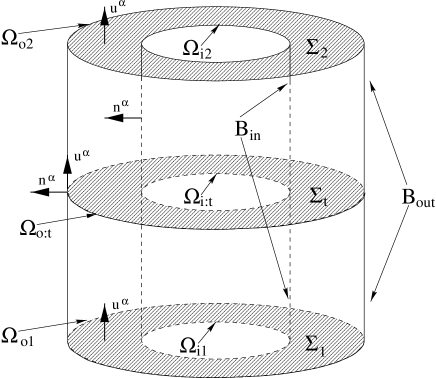
Figure 8: A three dimensional schematic showing the region $M$, its assorted boundary components, and the normals to those components.

We define a region of space-time $M$ as follows. Let ${\mathcal{M}}$ be a space-time and let $M\subset{\mathcal{M}}$ such that $\partial M$ consists of two space-like three surfaces $\Sigma_{1}$ and $\Sigma_{2}$ and two time- like three surfaces $B_{in}$ and $B_{out}$. These surfaces intersect as follows: $B_{out}\cap\Sigma_{1}=\Omega_{o1}$, $B_{in}\cap\Sigma_{1}=\Omega_{i1}$, $B_{out}\cap\Sigma_{2}=\Omega_{o2}$, $B_{in}\cap\Sigma_{2}=\Omega_{i2}$, $B_{in}\cap B_{out}=\emptyset$, and $\Sigma_{1}\cap\Sigma_{2}=\emptyset$.

Tensors in this space-time shall be labelled with greek indices. The metric tensor will be $g_{\alpha\beta}$ and the covariant derivative compatible with $g_{\alpha\beta}$ will be $\nabla_{\alpha}$. The Riemann tensor, Ricci tensor, Ricci scalar, and Einstein tensor will be ${\mathcal{R}}_{\alpha\beta\delta\gamma}$, ${\mathcal{R}}_{\alpha\beta}$, ${\mathcal{R}}$, and $G_{\alpha\beta}$ respectively.

Consider the time-like surfaces $B_{in}$ and $B_{out}$, starting with $B_{out}$. We define $n^{\alpha}$ to be the outward pointing space-like unit normal vector field on $B_{out}$. Then, we may define $\gamma^{\alpha}_{\;\;\beta}=\delta^{\alpha}_{\;\;\beta}-n^{\alpha}n_{\beta}$ as the projection tensor for $B_{out}$. Projecting the metric tensor onto $B_{out}$ we get the induced Lorentzian metric $\gamma_{\alpha\beta}=g_{\alpha\beta}-n_{\alpha}n_{\beta}$. The extrinsic curvature of this hypersurface in ${\mathcal{M}}$ is then defined as $\Theta_{\alpha\beta}=-\gamma^{\gamma}_{\;\;\alpha}\nabla_{\gamma}n_{\beta}$. The trace of $\Theta_{\alpha\beta}$ is $\Theta=g^{\alpha\beta}\Theta_{\alpha\beta}=\gamma^{\alpha\beta}\Theta_{\alpha\beta}$. The same notation will also be used to denote the corresponding quantities on $B_{in}$ (though in that case the normal vector field will point into $M$).

Next we consider the space-like surfaces $\Sigma_{1}$ and $\Sigma_{2}$ starting with $\Sigma_{2}$. We define $u^{\alpha}$ to be the outward pointing time-like unit normal vector field on $\Sigma_{2}$. Then the projection tensor is $h^{\alpha}_{\;\beta}=\delta^{\alpha}_{\;\beta}+u^{\alpha}u_{\beta}$ and the induced Euclidean signature metric on the surface is $h_{\alpha\beta}=h^{\delta}_{\;\alpha}h^{\epsilon}_{\;\beta}g_{\delta\epsilon}=g_{\alpha\beta}+u_{\alpha}u_{\beta}$. The compatible covariant derivative is $D_{\alpha}$. The extrinsic curvature of $\Sigma_{2}$ in ${\mathcal{M}}$ is $K_{\alpha\beta}=-h^{\gamma}_{\;\;\alpha}\nabla_{\gamma}u_{\beta}$, and its trace is $K=g^{\alpha\beta}K_{\alpha\beta}=h^{\alpha\beta}K_{\alpha\beta}$. The intrinsic Riemann tensor, Ricci tensor and scalar of the surface are $R_{\alpha\beta\gamma\delta}$, $R_{\alpha\beta}$, and $R$ respectively. Often, we shall tag tensors defined intrinsically on $\Sigma_{2}$ with lower case mid-alphabet indices (eg. $h_{ij}$, $K_{ij}$). Then the compatible covariant derivative will be $D_{i}$. The same notations will also be used to denote the corresponding quantities on $\Sigma_{1}$ (though in this case the unit normal vector will point into $M$).

Finally, we treat the intersection surfaces $\Omega_{o1}$, $\Omega_{o2}$, $\Omega_{i1}$, and $\Omega_{i2}$, starting with $\Omega_{o2}$. With loss of generality we shall make the standard assumption that on the $\Omega$ surfaces, $n^{\alpha}\bot u^{\alpha}$ (the non-orthogonal cases are partially discussed in [27] and [28] and will be discussed in more detail in [29]). Then, the projection operator onto the $\Omega$ surface is $\sigma^{\alpha}_{\;\;\beta}=\delta^{\alpha}_{\;\;\beta}+u^{\alpha}u_{\beta}-n^{\alpha}n_{\beta}$, and the induced metric is $\sigma_{\alpha\beta}=\sigma^{\alpha}_{\;\;\gamma}\sigma^{\beta}_{\;\;\delta}g_{\gamma\delta}=g_{\alpha\beta}+u_{\alpha}u_{\beta}-n_{\alpha}n_{\beta}$. If $\Omega_{o2}$ is viewed as a surface embedded in $\Sigma_{2}$ then it has an extrinsic curvature of $k_{\alpha\beta}\equiv-\sigma^{\alpha}_{\;\;\gamma}\sigma^{\beta}_{\;\;\delta}D_{\gamma}n_{\delta}$ with respect to $\Sigma_{2}$. The trace of $k_{\alpha\beta}$ is $k=g^{\alpha\beta}k_{\alpha\beta}=\sigma^{ij}k_{ij}$. The same notations will be used to denote the corresponding quantities on $\Omega_{o1}$, $\Omega_{i1}$, and $\Omega_{i2}$.

The next step of the programme is to define the surfaces of simultaneity - the “instants” of time. We decompose $M$ into a set of space-like hypersurfaces $\left\{\Sigma_{t}:t_{1}\leq t\leq t_{1}\right\}$ such that $\Sigma_{t_{1}}=\Sigma_{1}$ and $\Sigma_{t_{2}}=\Sigma_{2}$. On these surfaces we define the same quantities that were defined on $\Sigma_{1}$ and $\Sigma_{2}$. The same notation will be used for these quantities. The unit normals $u^{\alpha}$ are chosen to be consistently oriented with those on the boundary surfaces and we label the intersections with $B_{in}$ and $B_{out}$ as $\Omega_{o:t}=B_{out}\cap\Sigma_{t}$, $\Omega_{i:t}=B_{in}\cap\Sigma_{t}$. We extend our earlier orthogonality assumption so that on these intersection surfaces $u^{\alpha}n_{\alpha}=0$.

Finally, we define a flow of coordinate time on $M$. If $t$ is the hypersurface label, then we choose a vector field $t^{\alpha}$ such that $t^{\alpha}\nabla_{\alpha}t=1$. This vector field defines a flow. It may be decomposed into parts perpendicular and parallel to the hypersurfaces as

$$t^{\alpha}=Nu^{\alpha}+V^{\alpha},$$ (94)

where $N$ is called the lapse function and $V^{\alpha}$ is the shift vector which lies in the hypersurfaces (that is $u_{\alpha}V^{\alpha}=0$). Then the metric on $M$ may be decomposed

$$ds^{2}=-N^{2}dt^{2}+h_{ij}\left(dx^{i}+V^{i}dt\right)\left(dx^{j}+V^{j}dt\right),$$ (95)

as in section 4. It is then easy to show that

$\sqrt{-g}=N\sqrt{h}$, and $\sqrt{-\gamma}=N\sqrt{\sigma}$.

5.2 Analyzing the Action

The usual Einstein-Maxwell action with its boundary terms is,

$$I=-\frac{1}{2\kappa}\int_{M}d^{4}x\sqrt{-g}\left({\mathcal{R}}-2\Lambda-F^{2}\right)+\frac{1}{\kappa}\int_{\Sigma}d^{3}x\sqrt{h}K-\frac{1}{\kappa}\int_{B}d^{3}x\sqrt{-\gamma}\Theta.$$ (96)

We will work in the coordinate system where $c=\hbar=1$, and so $\kappa=8\pi$. Throughout this section an integral with subscript $B$ denotes two integrals - the indicated integral taken over $B_{out}$ minus the same integral over $B_{in}$. In the same way $\int_{\Sigma}=\int_{\Sigma_{2}}-\int_{\Sigma_{1}}$, $\int_{\Omega}=\int_{\Omega_{o2}}+\int_{\Omega_{i1}}-\int_{\Omega_{i2}}-\int_{\Omega_{o1}}$, and $\int_{\Omega_{t}}=\int_{\Omega_{o:t}}-\int_{\Omega_{i:t}}$.

Decomposing the action according to the foliation and time flow yields [10, 31]

$$I = -\int_{M}d^{4}x\left(P^{ij}\pounds_{t}h_{ij}-N{\mathcal{H}}-V^{i}{\mathcal{H}}_{i}-\frac{\sqrt{h}}{4\pi}E^{i}\pounds_{t}A_{i}+\frac{\sqrt{h}}{4\pi}A_{\alpha}t^{\alpha}{\mathcal{F}}_{el}\right)$$

$$+\int dt\int_{\Omega_{t}}d^{2}x\sqrt{\sigma}\left(N(\epsilon^{GR}+\epsilon^{EM})-V^{i}(j_{i}^{GR}+j_{i}^{EM})\right),$$

where $P^{ij}=\frac{\sqrt{h}}{16\pi}\left(Kh^{ij}-K^{ij}\right)$, $\pounds_{t}$ is the Lie derivative in the $t^{\alpha}$ direction, ${\mathcal{H}}$ and ${\mathcal{H}}_{a}$ are the Einstein-Maxwell constraints (1) and (2), and ${\mathcal{F}}_{el}$ is the electric Maxwell constraint (3). $A^{\alpha}$ is the electromagnetic vector potential, and may be broken up into its components perpendicular to and parallel to the hypersurfaces as $A^{\alpha}\equiv-\Phi u^{\alpha}+\tilde{A}^{\alpha}$. $\varepsilon^{GR}$ and $\varepsilon^{EM}$ are the energy densities of the gravitational and electromagnetic fields, while $j^{GR}_{a}$ and $j^{EM}_{a}$ are the angular momentum densities. Explicitly they are

$$\varepsilon^{GR} = \frac{k}{\kappa},$$ (98)

$$\varepsilon^{EM} = \frac{2\Phi E_{i}n^{i}}{\kappa},$$ (99)

$$j_{i}^{GR} = -\frac{2\sigma_{ij}n_{k}P^{jk}}{\sqrt{h}},\mbox{ and}$$ (100)

$$j_{i}^{EM} = \frac{2\tilde{A}_{i}E_{j}n^{j}}{\kappa},$$ (101)

where $E_{i}=e^{\alpha}_{i}F_{\alpha\beta}u^{\beta}$ is the electric field induced on the hypersurfaces. The interpretation of these quantities as energy and angular momentum densities is supported by calculations in the Schwarzschild and Kerr spacetimes [10, 31].

We may calculate the variation of $I$ with respect to $g_{\alpha\beta}$ (equivalently $N$, $V^{\alpha}$ and $h_{\alpha\beta}$), and $A_{\alpha}$ (equivalently $\Phi$ and $\tilde{A}_{a})$, as [10, 29]:

$$\delta I = -\frac{1}{2\kappa}\int_{M}d^{4}x\sqrt{-g}\left\{[G_{\alpha\beta}+\Lambda g_{\alpha\beta}-8\pi T^{EM}_{\alpha\beta}]\delta g^{\alpha\beta}-4[\nabla_{\alpha}F^{\alpha\beta}]\delta A_{\beta}\right\}$$

$$-\int_{\Sigma}d^{3}x\left\{P^{ij}\delta h_{ij}-\frac{2}{\kappa}\sqrt{h}E^{i}\delta\tilde{A}_{i}\right\}$$

$$-\int dt\int_{\Omega_{t}}d^{2}x\sqrt{\sigma}\left\{[\varepsilon^{GR}+\varepsilon^{EM}]\delta N-[j^{GR}_{i}+j^{EM}_{i}]\delta V^{i}-\frac{N}{2}s^{ij}\delta\sigma_{ij}\right\}$$

$$-\frac{1}{\kappa}\int dt\int_{\Omega_{t}}d^{2}xN\sqrt{\sigma}\left\{(n^{i}F_{ij}\sigma^{jk})\delta(\sigma^{l}_{\;\;k}\tilde{A}_{l})+(n^{i}E_{i})\delta\Phi\right\}.$$

In the above $T^{EM}_{\alpha\beta}$ is the standard electromagnetic stress energy tensor while $s^{ij}$ is the stress tensor for the surfaces $\Omega_{i/o:t}$. This tensor may written in terms of a trace-free shear $\eta^{ij}$ and pressure $p$ as

$$s^{ij}=\frac{p}{2}\sigma^{ij}+\eta^{ij},$$ (103)

while in turn the pressure and shear may be written as,

$$p = \frac{1}{\kappa}\left(2\frac{n^{i}\partial_{i}N}{N}-k\right),\mbox{ and}$$ (104)

$$\eta^{ij} = \frac{1}{\kappa}\left(k^{ij}-\frac{k}{2}\sigma^{ij}\right).$$ (105)

The last boundary term of $\delta I$ is purely electromagnetic and its components may be given a simple physical interpretation. To see this, recall that the electric and magnetic fields induced on the $\Sigma$ surfaces are

$$E_{\alpha} \equiv F_{\alpha\beta}u^{\beta}=\frac{1}{N}D_{\alpha}(N\Phi)-\pounds_{u}{\tilde{A}_{\alpha}},\mbox{ and}$$ (106)

$$B^{\alpha} \equiv -\frac{1}{2}\varepsilon^{\alpha\beta\gamma\delta}u_{\beta}F_{\gamma\delta}=-\varepsilon^{\alpha\beta\gamma\delta}u_{\beta}D_{\gamma}\tilde{A}_{\delta},$$

with respect to the field tensor $F_{\alpha\beta}$ and vector potential $A_{\alpha}$. Then we can see that $\sigma^{ij}\tilde{A}_{j}$ and $\Phi$ are necessary and sufficient to fix the component of $B_{i}$ perpendicular to the surfaces $\Omega_{t}$ and the components of $E_{i}$ parallel to those same surfaces. By contrast, $n^{i}F_{ij}\sigma^{jk}$ and $n^{i}E_{i}$ are necessary and sufficient to fix the perpendicular component of $E_{i}$ and the parallel components of $B_{j}$. A simple application of Gauss’s law of electromagnetism to the boundaries $\Omega_{t}$ of the regions $\Sigma_{t}$, then reveals that $\sigma^{ij}\tilde{A}_{j}$ and $\Phi$ are sufficient to fix the magnetic (but not electric) charge contained in the hypersurfaces $\Sigma_{t}$ while $n^{i}F_{ij}\sigma^{jk}$ and $n^{i}E_{i}$ are sufficient to fix the electric (but not magnetic) charge contained in the hypersurfaces.

We may find extremal points of the action functional by setting $\delta I=0$. Then, the two bulk terms of $\delta I$ respectively give us the Einstein-Maxwell equations. The remaining boundary terms specify quantities that must be fixed when we consider this particular action functional. Thus, in this case, the induced metric $h_{ij}$ and $\tilde{A}_{j}$ (and therefore the magnetic field) are fixed on the $\Sigma_{1}$ and $\Sigma_{2}$ surfaces, while the lapse $N$, shift $V^{i}$, induced metric $\sigma_{ij}$, $\sigma^{i}_{\ j}\tilde{A}_{i}$, and $\Phi$ are fixed on the boundaries $\Omega_{t}$. By the discussion of the previous paragraph, this means that we are considering paths with a fixed magnetic charge when we use this action functional.

We could change this situation if we chose to use the action functional $I_{electric}\equiv I+\Delta I_{electric}$, where

$$\Delta I_{electric}\equiv-\frac{1}{\kappa}\int_{\Sigma}d^{3}x\sqrt{h}F^{\alpha\beta}u_{\alpha}A_{\beta}+\frac{1}{\kappa}\int_{B}d^{3}x\sqrt{-\gamma}F^{\alpha\beta}n_{\alpha}A_{\beta},$$ (107)

instead. Solving $\delta I_{electric}=0$ we obtain the same equations of motion, but this time the purely electromagnetic boundary terms become

$$-\frac{2}{\kappa}\int_{\Sigma}d^{3}x\sqrt{h}\tilde{A}_{i}\delta E^{i}+\int dt\int_{\Omega_{t}}N\sqrt{\sigma}\left\{(\sigma^{\beta\gamma}\tilde{A}_{\gamma})\delta(n^{\alpha}F_{\alpha\beta}\sigma^{\beta\gamma})+\Phi\delta(n^{a}E_{a})\right\}.$$ (108)

Then, this modified action functional fixes the electric field on $\Sigma_{1}$ and $\Sigma_{2}$ and by equations (106) the electric (but not magnetic) charge on the $\Sigma_{t}$ hypersurfaces.

In a similar way we could (and in fact will) choose to fix the angular momentum of the paths considered by adding

$$\Delta I_{AngMom} = -\int dt\int_{\Omega_{t}}d^{2}x\sqrt{\sigma}V^{i}(j^{GR}_{i}+j^{EM}_{i})$$ (109)

to $I$. Then $(j^{GR}_{i}+j^{EM}_{i})$ rather than $V^{i}$ will be fixed on the $\Omega_{t}$ boundary surfaces. Hence the $\Sigma_{t}$ hypersufaces will all have the same total angular momentum. Thus with this modification to the action, paths contributing to the path integral will have fixed angular momentum.

5.3 Choosing an Action

Hence a choice of action entails a choice of boundary conditions that must be satisfied by solutions to the equations of motion. These boundary conditions are crucial to a correct application of the path integral formulation of gravity. A path integral with final conditions $X_{2}$ may be interpreted as a sum over all possible histories of a system leading up to the state $X_{2}$. Given this interpretation, and assuming that the state $X_{2}$ is in thermodynamic equilibrium, we may reinterpret the path integral as a thermodynamic partition function. Then the boundary conditions chosen along with an action become restrictions on which histories contribute to the partition function. The application of these restrictions then defines exactly which partition function we are studying – i.e. whether it is canonical, microcanonical, grand canonical, or some less standard partition function.

Pair creation calculations are typically carried out in the canonical partition function – that is where the temperature and all extensive variables (angular momentum, electric and/or magnetic charge) except for the energy are fixed [32]. This ensures that created spacetimes are in thermal equilibrium, that there is no discontinuity in physical properties such as electromagnetic charge and angular momenta at the juncture of the paths and the Lorentzian solution, and from a geometric point of view that the paths will smoothly match onto the Lorentzian solution. At first it might seem unusual that we do not choose to fix the energy, but support for this choice of partition function may be found if we examine the boundary conditions which must be imposed such that our interpolations will be smooth at the horizons.

At a non-degenerate horizon (i.e. both horizons of the lukewarm and Nariai instantons, the cosmological horizon for the cold instanton, and the single horizon for the ultracold I instanton) the paths will be closed and smooth if and only if $\tilde{N}=0$ and there are no conical singularities at those horizons. These conditions were discussed in some detail in section 4.3 for the actual instantons, and may be extended without difficulty to general paths. Recall that a conical singularity exists at a non-degenerate horizon at $r_{h}$ unless

$$\lim_{r\rightarrow r_{h}}\frac{\int_{0}^{P_{0}/2}dt\tilde{N}}{\int_{r_{h}}^{r}dr\sqrt{h_{rr}}}=\pi$$ (110)

This is equivalent to the condition

$$\lim_{r\rightarrow r_{h}}\frac{P_{0}\partial r\tilde{N}}{2\sqrt{h_{rr}}}=\pi$$ (111)

and so to ensure that all paths smoothly close at the horizons, this quantity must be fixed there. Since $\tilde{N}$ already vanishes at the horizon and since $n^{i}=\frac{1}{\sqrt{h_{rr}}}\frac{\partial}{\partial r}$, we see that this is exactly equivalent to fixing $\tilde{N}p$, where $p$ is the pressure defined in (104). Hence wherever we have a non-degenerate horizon we must add a boundary term

$$\Delta I_{pressure}=-\frac{1}{2}\int dt\int_{\Omega_{r_{h}:t}}d^{2}x\sqrt{\sigma}\tilde{N}p,$$ (112)

at that horizon in order for all paths to be smooth at those points. This has the effect of fixing the temperature at the horizon since (see section 3.7) constraining an interpolation to be regular at a horizon is equivalent to fixing the temperature there. Thus, for the two non-degenerate horizon spacetimes, geometric regularity demands that we fix the lapse $\tilde{N}$ and pressure $p$ (equivalently the temperature) rather than the energy densities.

Consider next the cold case with a degenerate black hole horizon. To match onto the Lorentzian solution all paths must have the “tapered horn” shape, with $\tilde{N}^{2}=0$ at the degenerate horizon. Since the horizon is an infinite proper distance from the rest of the space-time, there is no need to worry about conical singularities, and therefore no need to fix the pressure. Instead we leave $\sigma_{ij}$ fixed.

Since the ultracold spacetimes are limits of the other cases, we argue that where there are no natural boundaries (and thus we considered them to be at infinity) the $\tilde{N}$ must still be fixed at these inserted boundaries. Again where the space-time is not closed there is no need to fix the pressure since there is no chance of a conical singularity at those points.

To summarize, for the lukewarm, cold, and Nariai cases the imposition of regularity is equivalent to fixing the temperature, and therefore demanding that the created spacetimes be in thermal equilibrium. At the same time, we know that black holes are uniquely characterized by mass, angular momentum, and charge, so it is reasonable to demand of our interpolations that they have fixed angular momentum and charge. Fixing the mass is precluded since we must fix the temperature for the reasons discussed above.

The only boundary term of (5.2) that we have now not considered is the one on the $\Sigma_{2}$ surface that fixes $h_{ij}$. This is the natural quantity to fix in order to ensure that the paths will match onto the Lorentzian solutions. Thus, there is no need to add a boundary term in this situation.

As noted earlier, creation rates for these spacetimes will be proportional to the action of their corresponding instantons. As it stands, those rates are calculated only up to a normalization factor (see the discussion in section 2). Rather than calculate this multiplicative factor, we shall calculate the probability of their creation relative to that of deSitter space. This is given by

$$P=\exp{(2I_{deSitter}-2I)},$$ (113)

where $I$ is the action of the instanton, and $I_{deSitter}$ is the action of an instanton mediating the creation of deSitter space. Conventionally, this probability may also interpreted as the probability that deSitter space will tunnel into a given black hole space-time [26].

The space-like hypersurfaces of the spacetimes that we have considered are all of finite volume. In that case it is conventional [3, 32] to interpret them as having constant energy (even though we have not explicitly fixed this quantity with boundary conditions). Then, the canonical partition functions that we have considered would be equivalent to the microcanonical partition function and as is standard in thermodynamics we may calculate entropies as,

$$S=\ln{\Psi^{2}}=-2I.$$ (114)

With these factors in mind we turn to an evaluation of the actions.

5.4 Evaluating the Actions

Based on the above considerations, we see that the basic action that keeps the angular momentum, magnetic charge, and boundary lapses fixed is

$$I_{magnetic} = I+\Delta I_{AngMom}$$ (115)

$$= \left(\mbox{ terms that vanish for stationary solutions }\right)$$

$$+\int_{B}d^{3}x\sqrt{\sigma}N(\varepsilon^{GR}+\varepsilon^{EM}),$$

where $I$ is the action (5.2). In the above and in the following we have written the lapse in its Lorentzian form $N$ rather than its “Euclidean” form $\tilde{N}$. If we are evaluating one of these actions for an instanton, we substitute $\tilde{N}$ for $N$ in these expressions.

We note that in all of the cases that we consider, $N\varepsilon^{GR}=0$ on the boundaries where we evaluate it. Further, on those boundaries $N\varepsilon^{EM}$ turns out to be proportional to $E_{0}^{2}$. Thus, for magnetic instantons,

$$I_{magnetic}=0.$$ (116)

Of course extra boundary terms (the pressure terms) will have to be added to $I_{magnetic}$ for most of our instantons, so the total action will not be zero. We will come to these terms in a moment.

First however, we note that the basic action that keeps the angular momentum, electric charge, and boundary lapses fixed is

$$I_{electric} = I+\Delta I_{AngMom}+\Delta I_{electric}$$ (117)

$$= \left(\mbox{ terms that vanish for stationary solutions }\right)$$

$$+\int_{B}d^{3}xN\sqrt{\sigma}N(\varepsilon^{GR}+\varepsilon^{EM})-\frac{1}{\kappa}\int_{M}d^{4}x\sqrt{-g}F^{2}.$$

Since we will only be evaluating actions for instantons (whose accompanying electromagnetic fields are solutions of the Maxwell equations), we have used Stoke’s theorem to transform $\Delta I_{electric}$ (107) into a bulk term which is easier to evaluate. Now, as noted above $N\varepsilon^{GR}=0$ on the boundaries that we consider. Therefore, the basic action for electric instantons is

$$I_{electric}=\int_{B}d^{3}x\sqrt{\sigma}N\varepsilon^{EM}-\frac{1}{\kappa}\int_{M}d^{4}x\sqrt{-g}F^{2}.$$ (118)

As we shall see, in all of the cases that we consider these two terms will evaluate to be equal in magnitude but opposite in sign and so cancel each other out, leaving us with $I_{electric}=0$ again. Once again, the action will only be non-zero due to additional boundary terms.

These additional terms arise because it also is necessary to fix the pressure $p$ whenever there is a non-degenerate single horizon. In conjunction with fixing the lapse $N$ this ensures regularity of all paths at the horizon, sufficient to fix the temperature there as noted above.

Hence wherever there is a single, non-degenerate horizon, we must add the boundary term

$$\Delta I_{pressure}=-\frac{1}{2}\int_{B_{H}}d^{3}x\sqrt{\sigma}Np$$ (119)

to the action, where $B_{H}$ is the appropriate boundary corresponding to the horizon crossed with the time coordinate over the range $[0,\frac{P_{0}}{2}]$. From (104) we have $Np\rightarrow\frac{2}{\kappa}n^{k}\partial_{k}N$, and by (111), $n^{k}\partial_{k}N=\frac{2\pi}{P_{0}}$ on a non-degenerate horizon. Evaluating (119) by integrating over the instanton yields

$$\Delta I_{pressure}=-\frac{{\mathcal{A}}_{H}}{8}$$ (120)

where ${\mathcal{A}}_{H}$ is the surface area of the surface $\Omega_{H;2}$. Hence the action is equal to $-\frac{1}{8}$ times the sum of the areas of the non-degenerate horizons for all classes of instantons.

We give specific values for these quantities below (as well as the values of the cancelling terms in the electric actions).

Lukewarm Action: In this case, there are non-degenerate cosmological and outer black hole horizons. Therefore the total action of the magnetic instantons is

$$I_{MLW}=-\frac{{\mathcal{A}}_{c}+{\mathcal{A}}_{h}}{8}=-\frac{\pi(r_{c}^{2}+a^{2})}{2\chi^{2}}-\frac{\pi(r_{h}^{2}+a^{2})}{2\chi^{2}},$$ (121)

where ${\mathcal{A}}_{c}$ and ${\mathcal{A}}_{h}$ are respectively the areas of the cosmological and outer black hole horizons in the Lorentzian solution.

For the electric lukewarm instantons, we note that

$$\int_{0}^{\frac{P_{0}}{2}}d\tilde{t}\int_{\Omega_{\tilde{t}}}d^{2}x\sqrt{\sigma}\tilde{N}\varepsilon^{EM}=\frac{1}{\kappa}\int_{M}d^{4}x\sqrt{\tilde{g}}\tilde{F}^{2}=\frac{P_{0}E_{0}^{2}}{2\chi^{2}}\left(\frac{r_{c}}{r_{c}^{2}+a^{2}}-\frac{r_{h}}{r_{h}^{2}+a^{2}}\right),$$ (122)

and so the $I_{electric}=0$ as asserted, yielding

$$I_{ELW}=-\frac{\pi(r_{c}^{2}+r_{h}^{2}+2a^{2})}{2\chi^{2}}$$ (123)

for the total electric lukewarm action as well.

Nariai Actions: Again there are two non-degenerate horizons, this time at $\rho=\pm 1$. Therefore the total action of the magnetic Nariai instantons is

$$I_{MN}=-\frac{{\mathcal{A}}_{\rho=-1}+{\mathcal{A}}_{\rho=1}}{8}=-\frac{\pi(e^{2}+a^{2})}{\chi^{2}},$$ (124)

where ${\mathcal{A}}_{\rho=\pm 1}$ is the area of the horizon at $\rho=\pm 1$. We note that for the Nariai ${\mathcal{A}}_{\rho=1}={\mathcal{A}}_{\rho=-1}$.

For the electric Nariai instantons,

$$\int_{0}^{\frac{P_{0}}{2}}d\tilde{\tau}\int_{\Omega_{\tilde{\tau}}}d^{2}x\sqrt{\sigma}\tilde{N}\varepsilon^{EM}=\frac{1}{\kappa}\int_{M}d^{4}x\sqrt{\tilde{g}}\tilde{F}^{2}=-\frac{P_{0}E_{0}^{2}(e^{2}-a^{2})}{\chi^{2}(e^{2}+a^{2})}$$ (125)

and so the $I_{electric}=0$ as claimed. The total electric Nariai action is

$$I_{EN}=-\frac{\pi(e^{2}+a^{2})}{\chi^{2}},$$ (126)

equivalent to the magnetic case.

Cold Actions: Here there is only one non-degenerate horizon, and so

$$I_{MC}=-\frac{{\mathcal{A}}_{c}}{8}=-\frac{\pi(r_{c}^{2}+a^{2})}{2\chi^{2}},$$ (127)

where ${\mathcal{A}}_{c}$ is again the area of the cosmological horizon. Note that we consider the regions of the instanton to lie between $r=r_{c}$ and the degenerate horizon at $r=r_{h}$.

For the electric cold instantons the two terms of $I_{electric}$ take the same values that they did in the lukewarm case, and so $I_{electric}=0$ as promised. Hence the total electric cold action is given by

$$I_{EC}=-\frac{\pi(r_{c}^{2}+a^{2})}{2\chi^{2}}$$ (128)

as well.

Ultracold I Actions: Again there is only a single nondegenerate horizon, this time at $R=0$. The action of the magnetic ultracold I instanton is then

$$I_{MUCI}=-\frac{{\mathcal{A}}_{R=0}}{8}=-\frac{\pi(e^{2}+a^{2})}{2\chi^{2}}.$$ (129)

where this time the region we consider in our calculation is between $R=0$ and $R=R_{+}$. We shall take the limit $R_{+}\rightarrow\infty$ at the end of our calculation in order to include the whole instanton.

For the electric ultracold I instantons,

$$\int_{0}^{\frac{P_{0}}{2}}d\tilde{T}\int_{\Omega_{\tilde{T}}}d^{2}x\sqrt{\sigma}\tilde{N}\varepsilon^{EM}=\frac{1}{\kappa}\int_{M}d^{4}x\sqrt{\tilde{g}}\tilde{F}^{2}=-\frac{P_{0}E_{0}^{2}(e^{2}-a^{2})}{2\chi^{2}(e^{2}+a^{2})}R_{+}$$ (130)

so $I_{electric}=0$ as asserted, and

$$I_{EUCI}=-\frac{\pi(e^{2}+a^{2})}{2\chi^{2}}$$ (131)

as well.

Ultracold II Actions: There are no horizons whatsoever for this case, and so

$$I_{MUCII}=0,$$ (132)

irrespective of the chosen period $P_{0}$ of the “time” coordinate. We consider the region between $R=R_{-}$ and $R=R_{+}$, taking the limits $R_{-}\rightarrow-\infty$ and $R_{+}\rightarrow\infty$ at the end of the calculation to include the whole instanton.

For the electric ultracold II instantons,

$$\int_{0}^{\frac{P_{0}}{2}}d\tilde{T}\int_{\Omega_{\tilde{T}}}d^{2}x\sqrt{\sigma}\tilde{N}\varepsilon^{EM}=\frac{1}{\kappa}\int_{M}d^{4}x\sqrt{\tilde{g}}\tilde{F}^{2}=-\frac{P_{0}E_{0}^{2}(e^{2}-a^{2})}{2\chi^{2}(e^{2}+a^{2})}(R_{+}-R_{-}),$$ (133)

yielding $I_{electric}=0$ and so

$$I_{EUCII}=0,$$ (134)

as well.

In figure 9 we plot the above actions as a fraction of the action of the instanton creating deSitter space with the same cosmological constant. For all cases $I,I_{dS}<0$ and from the diagram we see that $|I|<|I_{dS}|$. Then $I_{dS}-I<0$ and we see that each of the space-times considered above is less likely to be created than deSitter space. Note that the Nariai space-time is the most likely to be created provided the parameter values are such that the instanton exists, while the cold space-time is the least likely to be created. As we might expect on physical grounds, smaller and more slowly rotating holes are more likely to be created than larger and more quickly rotating ones. As $\frac{a}{M}\rightarrow 0$ and $M\rightarrow 0$, the creation rates approach those of deSitter space.

Assuming that the space-times are at least quasi-static (see section 5.6 below), using equation (114) we see that the entropy of these space-times is equal to one- quarter of the sum of the areas of non-degenerate horizons bounding the Lorentzian region of the space-time. Consistent with [2] and [3], the degenerate horizon in the cold case does not contribute to the entropy of the cold space-time.

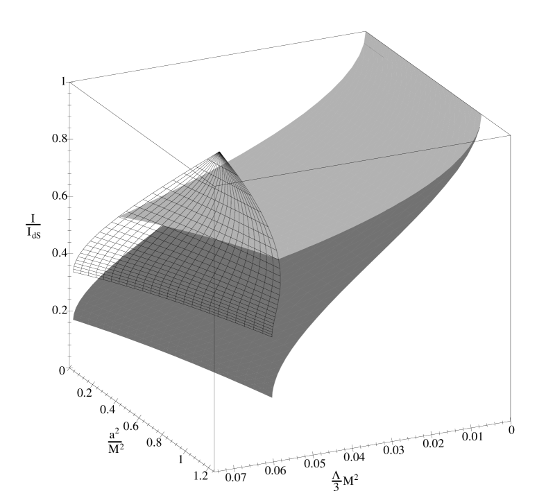
Figure 9: The actions for the charged and rotating lukewarm, cold, and Nariai instantons. The instantons are parameterized by $\frac{a^{2}}{M^{2}}$ and $\frac{\Lambda}{3}M^{2}$. Their actions are plotted as a fraction of the action $I_{dS}$ which is the action of the instanton creating pure deSitter space with the same cosmological constant. The Nariai instantons are the meshed sheet, the lukewarm instantons are the lighter grey sheet, and the cold instantons are the darker grey sheet.The ultracold I instanton actions may be found at the “bottom” end of the cold sheet, while the ultracold II instanton actions are zero.

5.5 Comparison to extant calculations

The approach we have taken in computing the instanton actions differs from those carried out for non-rotating black holes [3]. We pause to comment on the relationship between these cases.

In ref. [3] the fact that the instantons are closed and smooth at the points corresponding to the non-degenerate horizons was taken to mean that no boundary terms need be considered there, implying that the basic action used for the lukewarm and Nariai instanton should be

$$I_{old}=-\frac{1}{2\kappa}\int_{M}d^{4}x\sqrt{-g}\left({\mathcal{R}}-2\Lambda-F^{2}\right)-\frac{1}{\kappa}\int_{\Sigma}d^{3}x\sqrt{h}K,$$ (135)

which is our action (96) with the boundary term

$$\frac{1}{\kappa}\int_{B}d^{3}x\sqrt{-\gamma}\Theta$$ (136)

added on. It is easy to see that this term is equivalent to the pressure term

$$-\int_{B}d^{3}xN\sqrt{\sigma}\frac{p}{2}=-\int_{B}d^{3}xN\sqrt{\sigma}\left[\frac{n^{i}\partial_{i}N}{N}-\frac{k}{2}\right],$$ (137)

evaluated on the equivalent horizons. Noting that $\Theta=k-\frac{n^{i}\partial_{i}N}{N}$, and $k=-\frac{1}{2\sqrt{h_{rr}}}\partial_{r}\ln\sigma$, and $\frac{1}{\sqrt{h_{rr}}}\rightarrow 0$ at each horizon, we see that on the horizons $\Theta=-\frac{p}{2}$, and so in the non-rotating case our approach is equivalent to that of [3].

For the cold case $k$ still vanishes on the boundary and so the inclusion of the $\Theta$ term in [3] is the equivalent of the omission of the pressure term in our calculations. Finally, in the ultracold cases $k=0$ everywhere and so once more the omissions/inclusions are equivalent.

For electric instantons in both calculations electromagnetic boundary terms are added to the action to fix the electric charge for all paths considered in the path integral. Further, in both calculations for solutions to the Maxwell equations, these boundary terms may be converted into the $F^{2}$ bulk term that we have used.

Although for non-rotating instantons our approach is equivalent to earlier ones for evaluating the actions, differences arise when we include rotation. In earlier approaches [1, 2, 3, 4, 5, 6] there was no provision made for fixing the angular momentum.

The action differs by the term $\Delta_{AngMom}$ and its omission is tantamount to working with an incorrect thermodynamic ensemble. Evaluating the action of rotating instantons with (135) will not yield the preceding relationships linking surface areas, actions, and entropies. Indeed, using (135) the creation rate of rotating black holes is enhanced relative to that of non-rotating black holes and with an appropriate choice of physical parameters may be made arbitrarily large.

Recently Wu has considered the creation of a single black hole through the use of (slightly different) KNdS instantons [25]. Although we concur with the modifications that must be made to the action in order to properly take angular momentum into account, we disagree with the description of black hole creation presented. Creation of a single hole, as Wu considers, will not conserve angular momentum and electric/magnetic charge. Furthermore the instantons considered in that paper do not properly match to real Lorentzian solutions for two reasons. In the first place there are no periodic identifications of the universal covering space of the basic KNdS solution that can be made such that $t=\mbox{constant}$ hypersurfaces will contain only a single black hole. The smallest number of black holes that may be contained are the two that we have discussed in this paper. Second, as we have argued earlier, an analytic continuation of $a$ to $ia$ and $E_{0}$ to $iE_{0}$ will mean in general that an instanton generated from a classical solution will not properly match onto that classical solution: there will in general not even be the correct number of horizons available in the instanton to match onto the Lorentzian solution, and extrinsic curvatures, induced metrics, and induced electromagnetic fields will not match across a $t=\mbox{constant}$ surface.

5.6 Issues of Equilibrium II

Finally we return briefly to the discussion in section 3.7. Recall that the spacetimes of the pair-created black holes are in thermal equilibrium, but not in equilibrium with respect to the charged particle creation and super-radiance effects. These will cause the black hole spacetimes to discharge and/or spin down.

This problem is also present (at least in principle) in previous work on charged black hole pair-creation [1, 2, 3, 6, 17]) since in those cases charged black holes tend to discharge via charged particle creation effects.

The first, and more conservative response to this situation, is to argue that even if the created spacetimes are not static (in the thermodynamic sense), then perhaps their evolution is slow enough that they may be viewed as quasistatic. In section 3.7 we saw that there is some evidence for this point of view in the literature, though admittedly our current situation has not been explicitly addressed. It seems clear however that at least some finite class of the spacetimes that we have considered will be close enough to equilibrium that the calculations will be correct to the first order of approximation. In a future paper we will explore this quantitatively.

An alternate (and more radical) response is to argue that only thermal equilibrium (in the sense of equal temperatures at the horizons) is needed for pair creation. Here we would argue that while the requirement of thermal equilibrium arises naturally from the smoothness conditions on the instantons, the extra requirements of full thermodynamic equilibrium do not arise naturally from such conditions and are instead imposed from outside. Of course on physical grounds we would expect that full thermodynamic equilibrium would be required, but it at least seems possible that this might not be the case. For now we will leave this issue open.

6 Discussion

We have demonstrated the physical process of creation of static black hole pairs via cosmological vacuum energy may be extended to the creation of stationary black hole pairs. Although the calculation is somewhat more subtle and complicated, the basic results continue to hold qualitatively. Just as there are static lukewarm, cold, Nariai, and ultracold instantons describing pair-creation in a cosmological (or for that matter electromagnetic [1]) background, so also are there the same classes of instantons for rotating black hole pairs. Furthermore, the entropy of such spacetimes continues to be proportional to the sum of the areas of the horizons in the standard manner, and pair creation rates continue to be proportional to the exponential of those entropies and suppressed relative to the creation of a pure deSitter space.

In order to describe this process we have had to depart from the usage of purely real Euclidean instantons and consider complex instantons. This followed from a consideration of the standard matching conditions required in the Euclidean gravity formalism which specify that instantons must smoothly match to their corresponding Lorentzian solutions. Demanding that rotating instantons be real implies they will no longer match onto their Lorentzian counterparts. Although it is somewhat unusual to introduce complex metrics, our results are consistent with the interpretation of the functional integral formalism for black hole thermodynamics discussed in ref.[9].

A second departure from the standard techniques arises due to the boundary terms we must add when rotation is present. In pair-creation calculations for non-rotating black holes, one uses the basic Einstein-Maxwell action (96), and we have seen that this action is equivalent to the one that we have used. However it must be modified by additional boundary terms when rotation is present in order to appropriately fix angular momentum on the matching surface, somewhat analogous to the situation in which boundary terms must be added in the electric case in order to maintain electromagnetic duality [32, 30]. Usage of (96) for rotating cases yields the unphysical result that pair-creation of rotating holes is enhanced rather than suppressed relative to deSitter space.

Finally, we have seen that thermal equilibrium does not necessarily correspond to thermodynamic equilibrium. The question as to which is the correct requirement to put on spaces that are to be created by quantum tunnelling has been left open. Geometrically it would appear that only thermal equilibrium is required, but on physical grounds we would expect full thermodynamic equilibrium to be required. We have suggested that even if full thermodynamic equilibrium is required, then at least a class of the spacetimes that we have discussed will be close enough to equilibrium to be considered quasistatic, in which case the approximate entropies and pair creation rates should still be correct.

References

- [1] H.F. Dowker, J.P. Gauntlett, D.A. Kastor and J. Traschen, Phys. Rev. D49, 2909 (1994); H.F. Dowker, J.P. Gauntlett, S.B. Giddings and G.T. Horowitz, Phys. Rev. D50, 2662 (1994); D. Garfinkle, S.B. Giddings and A. Strominger, Phys. Rev. D49, 958 (1994).
- [2] S.W. Hawking, G.T.Horowitz, and S.F. Ross, Phys. Rev.D51, 4302 (1995).
- [3] R.B. Mann and S.F. Ross, Phys. Rev.D52, 2254 (1995).
- [4] R. Bousso and S.W. Hawking, Phys. Rev.D54, 6312 (1996).
- [5] S.W. Hawking and Simon F. Ross, Phys. Rev. Lett. 75 (1995) 3382; R. Emparan Phys. Rev. Lett. 75 (1995) 3386 ; D. Eardley, G. Horowitz, D. Kastor and J. Traschen, Phys. Rev. Lett. 75 (1995) 3390.
- [6] R.R. Caldwell, G.W. Gibbons, and A. Chamblin, Phys. Rev. D53 (1996) 7103; R. B. Mann, Class. Quantum Grav. 14 (1997) L109; R.B. Mann, Nucl. Phys. B516 (1998) 357.
- [7] J.F. Plebanski and M. Demianski, Ann. Phys. (N.Y.) 98, 98, (1976).
- [8] G.W. Gibbons and S.W. Hawking, Comm. Math. Phys. 66 (1979) 291.
- [9] J.D. Brown, E.A. Martinez and J.W. York, Phys. Rev. Lett. 66 (1991) 2281.
- [10] J.D. Brown and J.W. York, Phys. Rev.D47, 1407–1420; 1420–1431 (1993); gr-qc/9405024.
- [11] G.W. Gibbons and S.W. Hawking, Phys. Rev.D15, 2752 (1977).
- [12] J.B. Hartle and S.W. Hawking, Phys. Rev.D28, 2960 (1983).
- [13] W. Kinnersley and M. Walker, Phys. Rev.D2, 1359 (1970).
- [14] F. Mellor and I. Moss, Class. Quantum Grav.6, 1379 (1989).
- [15] G.W. Gibbons and S.W. Hawking, Phys. Rev.D15, 2738 (1977).
- [16] P. Ginsparg and M.J. Perry, ,Nucl. Phys.B222, 245 (1983).
- [17] R. Bousso, Phys. Rev.D55, 3614 (1997).
- [18] S.W. Hawking, Nature 248, 30 (1974).
- [19] G.W. Gibbons, Commun. Math. Phys.44, 245 (1995).
- [20] D.N. Page, Phys. Rev.D13, 198 (1976).
- [21] D.N. Page, Phys. Rev.D14, 3260 (1976).
- [22] C.M. Chambers, W.A. Hiscock, and B.T. Taylor, Phys. Rev. Lett.78, 3249, (1997).
- [23] T. Tachizawa and K. Maeda, Phys. Lett.A172, 325 (1993).
- [24] A.S. Lapedes and J.P. Perry, Phys. Rev.D24, 1981 (1981).
- [25] Z.C. Wu, Int. J. Mod. Phys. D6 199 (1997).
- [26] R. Bousso and A. Chamblin, gr-qc/9803047.
- [27] S.W. Hawking and C.J. Hunter, Class. Quantum Grav.13, 2735 (1996).
- [28] G. Hayward Phys. Rev.D47, 3275 (1993).
- [29] I.S. Booth and R.B. Mann, gr-qc/9806015 (to appear Phys. Rev.D), and manuscript in preparation.
- [30] J.D. Brown Phys. Rev.D56, 1001 (1997).
- [31] S.W. Hawking and G.T. Horowitz, Class. Quantum Grav.13, 1487 (1996).
- [32] S.W. Hawking and S.F. Ross, Phys. Rev.D52, 5865 (1995).