Abstract

We analyze here the issue of local versus the global visibility of a singularity that forms in gravitational collapse of a dust cloud, which has important implications for the weak and strong versions of the cosmic censorship hypothesis. We find conditions as to when a singularity will be only locally naked, rather than being globally visible, thus preseving the weak censorship hypothesis. The conditions for formation of a black hole or naked singularity in the Szekeres quasi-spherical collapse models are worked out. The causal behaviour of the singularity curve is studied by examining the outgoing radial null geodesics, and the final outcome of collapse is related to the nature of the regular initial data specified on an initial hypersurface from which the collapse evolves. An interesting feature that emerges is the singularity in Szekeres spacetimes can be “directionally naked”.

1 Introduction

An important question regarding the final configurations resulting out of gravitational collapse of massive matter clouds is, in case a naked singularity develops rather than a black hole, whether it would be visible to a far away observer or not. This issue of local versus global visibility of the singularity has important implications for the cosmic censorship principle. Whenever naked singularities formed, if they were only locally naked rather than being globally visible, that would mean the weak cosmic censorship would hold, even though the strong censorship may be violated [1]. In its strong version the cosmic censorship states that singularities cannot be even locally visible, whereas the weak formulation allows for the singularities to be at least locally naked, but requires that they should not be globally naked.

If the naked singularities formed but were always only locally naked and not visible to far away observers outside the event horizon, then though the strong form is violated, the validity of the weak version has the astrophysical implication that far away observers may never see the emissions from the singularity, or the very dense strong curvature regions near the same. This effectively seals the singularity inside the black hole. Thus, given a gravitational collapse scenario, it is of importance to determine if the singularity forming could be only locally naked, and if so under what conditions. On the other hand, if the singularity is globally visible, thus accessible to the outside observers, one would like to ascertain the conditions under which this would be possible, and to relate these to the nature of regular initial data from which the collapse develops.

Our purpose here is to analyze a wide class of collapse models, namely the quasi-spherical spacetimes given by Szekeres[2], from such a perspective. Such an investigation is also of additional interest because these models are not spherically symmetric. The non-solvability of Einstein equations restrict most of the studies of formation and structure of singularities in gravitational collapse limited to spherically symmetric models, and a simple enough equation of state, namely $p=0$. Though results on some specific solutions are available for more general equation of state $p=k\rho$[3], still most of the work considering departures from spherical symmetry is numerical (see e.g. [4]). Analytic study of collapsing models with more general geometries is of considerable interest since strict spherical symmetry is a strong assumption. Thus we study here the formation of singularities in the Szekeres spacetimes, which do not admit any Killing vectors but allow an invariant family of two spheres, and has the Tolman-Bondi-Lemaître (TBL) model [5] as its special case. In a recent paper Joshi and Królak [6] have shown existence of naked singularities in these models. Here we analyze the situation further to relate the formation of naked singularities or black holes with the initial data from which the collapse develops. The transition between the black hole and naked singularity phase is shown to be related to the nature of the initial data, and we also examine how the local versus the global visibility of the naked singularity changes with the change of essential parameters in the initial data.

In section 2 we briefly review the Szekeres model. In sections 3 and 4, we derive the necessary and sufficient condition for the existence of outgoing radial null geodesics (RNGs) from the singularity, and we relate the formation of naked singularities with the regular data specified on the initial hypersurface. In section 5, we investigate numerically the conditions for the global nakedness of the singularity in the TBL and Szekeres spacetimes. The final section 6 outlines some conclusions.

2 Quasi-spherical gravitational collapse

The metric in a comoving coordinate system has the form,

$$ds^{2}=dt^{2}-M^{2}dr^{2}-N^{2}(dx^{2}+dy^{2}),$$ (1)

The energy-momentum tensor is of the form of an irrotational dust,

$$G^{ij}=T^{ij}=\epsilon\delta^{i}_{t}\delta^{j}_{t},$$ (2)

where $\epsilon(t,r)$ is the energy density of the cloud (here units are chosen such that $c$ = $8\pi G$ = 1). For convenience we adopt a pair of complex conjugate coordinates, $\zeta=x+iy,\;\;\;\bar{\zeta}=x-iy,$ in which the metric takes the form

$$ds^{2}=dt^{2}-M^{2}dr^{2}-N^{2}d\zeta d\bar{\zeta}$$ (3)

Where M and N are general functions of $t,r,\zeta$ and $\bar{\zeta}$. The integrated form of Einstein’s equations is given by Szekeres[2],

$$N={{R(r,t)}\over{Q(r,\zeta,\bar{\zeta)}}},~{}~{}~{}~{}M={{QN^{\prime}}\over{\sqrt{1+f}}},$$ (4)

restricted to the case, $N^{\prime}\equiv{{\partial N}\over{\partial r}}\neq 0$, where the prime and dot denote partial derivatives with respect to $r$ and $t$ respectively. Here $f(r)$ is an arbitrary function of $r$ subject to the restriction $f>-1,$ and $Q(r,\zeta,\bar{\zeta})$ is of the form

$$Q=a(r)\zeta\bar{\zeta}+B(r)\zeta+\bar{B}(r)\bar{\zeta}+c(r).$$ (5)

Here $a$ and $c$ are arbitrary real functions and $B$ is a complex function of $r$, satisfying

$$ac-B\bar{B}={\delta\over 4},\;\;\delta=\pm 1\;,\;0.$$ (6)

We will consider here the case $\delta=+1$. In this case it is possible to reduce the two-metric by a bilinear transformation of coordinates $\zeta,\bar{\zeta}$ to the form,

$$R^{2}(r,t)d\zeta d\bar{\zeta}/{1\over 4}(\zeta\bar{\zeta}+1)^{2},$$ (7)

which, on subsequent introduction of polar coordinates $\zeta=e^{i\varphi}\cot{1\over 2}\theta,~{}~{}\bar{\zeta}=e^{-i\varphi}\cot{1\over 2}\theta,$ reduces (7) to the normal form of metric on a two-sphere given by $R^{2}(r,t)(d\theta^{2}+\sin^{2}\theta d\varphi^{2}).$ Hence, the two-surfaces $S_{r,t}$ defined by $t=const.,r=const.$ are spheres of radius $R(r,t)$. Here $R(r,t)$ satisfies the “Friedmann equation”

$$\dot{R}^{2}=f(r)+{{F(r)}\over R},$$ (8)

which is similar to the equation holding for the TBL models. Since we are studying collapse scenarios, we consider the collapsing branch of the solution, i.e. $\dot{R}\leq 0$. One more free function, corresponding to the epoch of singularity formation, arises when one integrates the above equation and we get

$$\int(f(r)+\frac{F(r)}{R})^{-1/2}dR=t-t_{0}(r)$$

Functions $F$ and $f$ are arbitrary functions of $r$, and $t_{0}(r)$ is another free function, which can be fixed using the scaling freedom. The density is given by,

$$\rho={{QF^{\prime}-3FQ^{\prime}}\over{R^{2}(QR^{\prime}-RQ^{\prime})}}.$$ (9)

Therefore, the singularity curve is given by

$$R(r,t_{0})=0,\;\;\;\;(t_{0}>t_{i}),$$ (10)

$$Q(r,t_{sc},\zeta)R^{\prime}(r,t_{sc})-R(r,t_{sc})Q^{\prime}(r,t_{sc},\zeta)=0,\;\;(t_{sc}>t_{i}).$$ (11)

Here $t_{i}$, $t_{0}$ and $t_{sc}$ give the times corresponding to that of the regular initial hypersurface, and the shell-focusing and shell-crossing singularities respectively.

To analyze the shell-focusing singularity, it is essential to choose the initial data in such a way that $t_{i}<t_{0}<t_{sc}$. The range of coordinates is given by

$$R\neq 0,\;\;\;\;Q(r,t,\zeta)R^{\prime}(r,t)-R(r,t)Q^{\prime}(r,t,\zeta)\neq 0$$ (12)

We can easily check that if the functions $a(r)$, $B(r)$, $\bar{B}(r)$, and $c(r)$ are constants then the equation (9) reduces to the corresponding equation for the TBL metric. Amongst the functions $a$, $c$, $B$, $\bar{B}$, $F$, $f$ and $t_{0}(r)$, equation (6) and a gauge freedom would leave total five free functions in general. In comparison to the TBL models, where we have only two free functions, namely $F(r)$ (the mass function) and $f(r)$ (the energy function), this model is clearly functionally more generic, allowing for a certain mode of non-sphericity to be included in the consideration.

3 Gravitational collapse and singularity formation

Assuming the validity of Einstein’s equations, the singularity theorems[7] ensure the formation of singularity in gravitational collapse if some reasonable conditions are satisfied by the initial data. For analyzing the detailed structure of the singularity curve, integrating equation (8) we get

$$t-t_{0}(r)=-{{R^{3/2}G(-fR/F)}\over{\sqrt{F}}},$$ (13)

where $G(y)$ is a strictly convex, positive function having the range $1\geq y\geq-\infty$ and is given by

$$G(y)=\cases{{{\rm arcsin}\sqrt{y}\over y^{3/2}}-{\sqrt{1-y}\over y},&$1\geq y>0$,\cr{2\over 3},&$y=0$,\cr{-{\rm arcsinh}\sqrt{-y}\over(-y)^{3/2}}-{\sqrt{1-y}\over y},&$0>y\geq-\infty$.\cr}$$ (14)

Here $t_{0}(r)$ is a constant of integration. Using the scaling freedom, we can choose

$$R(0,r)=r,$$ (15)

and this gives

$${t_{0}(r)=}{{r^{3/2}G(-fr/F)}\over{\sqrt{F}}},$$ (16)

i.e. the singular epoch is uniquely specified in terms of the other free functions. The function $t_{0}(r)$ gives the time at which the physical radius of the shell labeled by $r=$ const. becomes zero, and hence the shell becomes singular.

The quantity $R^{\prime}$ which is useful for the further analysis, can be expressed using equations (13-16) as

$$\begin{array}[]{clcr}R^{\prime}=&r^{\alpha-1}[(\eta-\beta)X+[\Theta-(\eta-\frac{3}{2}\beta)X^{3/2}G(-PX)]\times[P+\frac{1}{X}]^{1/2}]\\ ~{}~{}~{}~{}\equiv&r^{\alpha-1}H(X,r),\end{array}$$ (17)

where we have used

$$u=r^{\alpha},\;X=(R/u),\;\eta(r)=r\frac{F^{\prime}}{F},\;\;\beta(r)=r\frac{f^{\prime}}{f},\;\;p(r)=r\frac{f}{F},\;\;P(r)=pr^{\alpha-1},\;\;$$

$$~{}~{}~{}\Lambda=\frac{F}{r^{\alpha}},\;\;\;\Theta\equiv\frac{t^{\prime}_{s}\sqrt{\Lambda}}{r^{\alpha-1}}=\frac{1+\beta-\eta}{(1+p)^{1/2}r^{3(\alpha-1)/2}}+\frac{(\eta-\frac{3}{2}\beta)G(-p)}{r^{3(\alpha-1)/2}}.$$ (18)

The function $\beta(r)$ is defined to be zero when $f=0$. All the quantities defined here are such that while approaching the central singularity at $r=0$ they tend to finite limits, thus facilitating a clearer analysis of the singular point. The factor $r^{\alpha}$ has been introduced for analyzing geodesics near the singularity. The constant $\alpha(\geq 1)$ is determined uniquely using the condition that $\Theta(X,r)$ goes to a nonzero finite value in the limit $r$ approaching $0$ along any $X$ = constant direction. The angular dependence in the metric appears through $\xi,\bar{\xi}$ and along radial null geodesics $\xi\bar{\xi}=$const.

Using the metric (3), the equation for the RNGs is,

$${{dt}\over{dr}}={{QR^{\prime}-RQ^{\prime}}\over{Q\sqrt{1+f}}}.$$ (19)

Which in terms of $R$ and $u=r^{\alpha}$ can be rewritten as

$${{dR}\over{du}}={{1}\over{\alpha r^{\alpha-1}}}{\biggr{[}}\dot{R}{{dt}\over{dr}}+R^{\prime}{\biggr{]}}={{\biggr{[}}{1-{{\sqrt{f+\Lambda/X}}\over{{\sqrt{1+f}}}}(1-{{RQ^{\prime}}\over{QR^{\prime}}}){\biggr{]}}}{{H(X,u)}\over{\alpha}}},~{}~{}~{}~{}~{}~{}~{}~{}~{}~{}~{}~{}~{}~{}~{}$$

$$~{}~{}~{}~{}~{}~{}~{}~{}\equiv U(X,u)+{{H(X,u)}\over{\alpha}}{{\sqrt{f+\Lambda/X}}\over{{\sqrt{1+f}}}}{{RQ^{\prime}}\over{QR^{\prime}}}.$$ (20)

For spherically symmetric models we get $Q^{\prime}=0$, and the above equation reduces to the TBL case. The point $u=0$, $R=0$ is a singularity of the above first order differential equation. To study the characteristic curves of the above differential equation, we define $X=R/r^{\alpha}=R/u$. For the outgoing RNGs, $dR/du>0$ is a necessary condition. If future directed null geodesics meet the first singularity point in the past with a definite value of the tangent ($X=X_{0}$), then using equation (20) and l’Hospital’s rule, we can write for that value $X_{0}$,

$$X_{0}=\lim_{R\to 0,u\to 0}{{R}\over{u}}=\lim_{R\to 0,u\to 0}{{dR}\over{du}}=\lim_{R\to 0,u\to 0}{{\biggr{[}}{1-{{\sqrt{f+\Lambda/X}}\over{{\sqrt{1+f}}}}(1-{{RQ^{\prime}}\over{QR^{\prime}}}){\biggr{]}}}{{H(X,u)}\over{\alpha}}}.$$ (21)

Since $Q(0)\neq 0$, $Q^{\prime}(0)=0$ and near the central singularity $R^{\prime}\propto R/r$, if there is a definite tangent to the RNGs coming out, we can neglect $(RQ^{\prime})/(QR^{\prime})$ near the first singular point. Therefore the result is similar to the TBL model[8],

$$X_{0}=\lim_{{r\to 0},{u\to 0}}U(X,r)=U(X_{0},0).$$ (22)

We have introduced here the notation that a subscript zero on any function of $r$ denotes its value at $r=0$. Defining

$$V(X)=U(X,0)-X={{\biggr{[}}{1-{{\sqrt{f_{0}+\Lambda_{0}/X}}\over{{\sqrt{1+f_{0}}}}}{\biggr{]}}}}{{H(X,0)}\over{\alpha}}-X,$$ (23)

the existence of a real positive value $X=X_{0}$ for the above equation such that

$$V(X_{0})=0,$$ (24)

gives a necessary condition for the singularity to be at least locally naked.

In the neighborhood of the singularity we can write $R=X_{0}r^{\alpha}$, where $X_{0}$ is positive real root of above equation. To check whether the value $X_{0}$ is actually realized along any outgoing singular geodesic, we consider the equation for RNGs in the form $u=r^{\alpha}=u(X)$. From equation (20) we have

$${{dX}\over{du}}={1\over{u}}{{\bigg{[}}{{{dR}\over{du}}-X}{\bigg{]}}}={1\over{u}}{{\bigg{[}}{U(X,u)-X+({{\sqrt{f+\Lambda/X}}\over{\sqrt{1+f}}}){{XQ^{\prime}u^{1/\alpha}}\over{\alpha Q}}}{\bigg{]}}}.$$ (25)

The third term on the right hand side goes to zero faster than the first near $r=0$. The solution of the above equation gives the RNGs in the form $u=u(X)$. Now if the equation $V(X)=0$ has $X=X_{0}$ as a simple root, then we can write

$$V(X)\equiv(X-X_{0})(h_{0}-1)+h(X),$$ (26)

where

$$h_{0}={1\over{H_{0}}}{{\bigg{[}}{{{\Lambda_{0}H_{0}^{2}}\over{2\alpha X_{0}^{2}\sqrt{f_{0}+\Lambda_{0}/X_{0}}\sqrt{1+f_{0}}}}+{{X_{0}N_{0}}\over{\sqrt{f_{0}+\Lambda_{0}/X_{0}}}}}{\bigg{]}}},$$ (27)

is a constant and the function $h(X)$ is chosen in such a way that

$$h(X_{0})={{\bigg{[}}{{dh}\over{dX}}{\bigg{]}}}_{X=X_{0}}=0,$$ (28)

i.e. $h(X)$ contains higher order terms in $(X-X_{0})$ and $H_{0}=H(X_{0},0)$, $N_{0}=N(X_{0},0)$ with $N(X,r)=-\dot{R}^{\prime}r$.

As we are studying RNGs, $Q$ and $Q^{\prime}$ are just the functions of $r$ (i.e. $u$), therefore the equation for $dX/du$ can be written as

$${{dX}\over{du}}-(X-X_{0}){{h_{0}-1}\over u}={S\over u}$$ (29)

Here the function

$$S=S(X,u)=U(X,u)-U(X_{0})+h(X)+{{\sqrt{f+\Lambda/X}}\over{\sqrt{1+f}}}({{XQ^{\prime}u^{1/\alpha}}\over{\alpha Q}})$$ (30)

is such that $S(X_{0},0)=0$. Note that unlike the TBL case, here $S$ also has some functional dependence on $\zeta$ and $\bar{\zeta}$. We can take care of this by considering radial geodesics, i.e. only those with fixed $\zeta$ and $\bar{\zeta}$. Multiplying equation (29) by $u^{-h_{0}+1}$ and integrating we get

$$X-X_{0}=Du^{h_{0}-1}+u^{h_{0}-1}\int Su^{-h_{0}}du,$$ (31)

where $D$ is a constant of integration that labels different geodesics. We see from this equation that the RNG given by $D=0$ always terminates at the singularity $R=0,u=0$, with $X=X_{0}$ as the tangent. Also, for $h_{0}>1$, a family of outgoing RNGs terminates at the singularity with $X=X_{0}$ as the tangent. Therefore the existence of a real positive root to equation (24) is also a sufficient condition for the singularity to be at least locally naked.

Near the singularity the geodesic equation can be written as

$$X-X_{0}=Du^{h_{0}-1}.$$

Hence for $h_{0}>1$ there is an infinite family of RNGs which terminate at the singularity in the past with $X_{0}$ as a tangent. For $h_{0}\leq 1$ there is only one RNG corresponding to $D=0$ which terminates at the singularity with $X_{0}$ as a tangent. In ($R$,$u$) plane

$$R-X_{0}u=Du^{h_{0}},$$

and for $h_{0}>1$ we have a family of infinitely many outgoing RNGs meeting the spacetime singularity in the past. For $h_{0}\leq 1$ only $D=0$ geodesic terminates at the physical singularity ($t_{0}(0),u=0$) in the past.

A relevant question is, if only one RNG has the tangent $X=X_{0}$ in the (u,R) plane then what is the behaviour of the RNGs which are inside this root and very close to the singularity? They cannot cross the root so they have to start from the singularity in the past. And if they are outside the apparent horizon, then certainly the only possible tangent they can have at the singularity is the same as the tangent made by the apparent horizon at the singularity. To check if our differential equation for RNGs can satisfy this near the singularity, we note that in equation (20) the term in the bracket goes to zero, while $H$ blows up in this limit. In the limit to the singularity, we expect $R/r^{3}$ to be $F_{0}$ along the RNG. To the lowest order we assume that along the RNG

$$R=F+M_{\delta}r^{\delta+3}$$

and check for the consistency by determining $M_{\delta}$ and $\delta$ in the limit. For the $f=0$ case, using l’Hospital’s rule we get,

$$F_{0}=\lim_{R\to 0,r\to 0}{{R}\over{r^{3}}}=\lim_{R\to 0,r\to 0}{{dR}\over{d(r^{3})}}=\lim_{R\to 0,r\to 0}{{\bigg{[}}1-\sqrt{F/R}{\bigg{]}}}{\bigg{[}}X+{1\over{\sqrt{X}}}{{nF_{n}}\over{F_{0}}}r^{n-3}{\bigg{]}}$$

$$\;\;~{}~{}~{}~{}~{}~{}=\lim_{R\to 0,r\to 0}{{1\over 6}{{nM_{\delta}F_{n}\over{{F_{0}}^{5/2}}}r^{\delta+n-3}}},$$ (32)

where $X=R/r^{3}$. This leads to,

$$\delta=3-n\;~{}and~{}\;M_{\delta}=-{{6{F_{0}}^{7/2}}\over{nF_{n}}}.$$

That means that our assumption is consistent. One can also check that any other kind of behavior of the RNGs near the singularity is not possible.

4 End state of quasi-spherical dust collapse

In this section, we analyze the end state of quasi-spherical dust collapse evolving from a given regular density and velocity profile. Our purpose here is to determine how a given initial profile influences and characterizes the outcome of the collapse. We will be mainly studying the marginally bound ($f=0$) case for convenience. The results can be generalized to non-marginally bound case using an analysis similar to that developed by Jhingan and Joshi[9] for the case of TBL models.

The initial density profile for a fixed radial direction ($\zeta$ and $\bar{\zeta}$ are constant) is given by $\rho=\rho(r)$, and if we are given the function $Q$ then it is possible in principle to find out the function $F(r)$ from the density equation (9). In order to give a physically clear meaning to our results, we assume all the functions (i.e. $\rho$, $Q$, and $F$ ) to be expandable in $r$ around the $r=0$ point on the initial hypersurface. This means that even though the functions are expandable, we do not necessarily require them to be $C^{\infty}$ and smooth. Therefore we take

$$\rho=\sum_{n=0}^{\infty}\rho_{n}r^{n},$$ (33)

$$Q=\sum_{n=0}^{\infty}Q_{n}r^{n}~{}~{}~{}~{}~{}~{}~{}~{}Q_{0}\neq 0,$$ (34)

where the regularity condition implies $Q_{1}=0$ [2], and

$$F=\sum_{n=0}^{\infty}F_{n}r^{n+3}.$$ (35)

Therefore

$$Q^{\prime}=\sum_{n=2}^{\infty}nQ_{n}r^{n-1},$$ (36)

and,

$$F^{\prime}=\sum_{n=0}^{\infty}(n+3)F_{n}r^{n+2}.$$ (37)

Substituting the values of these functions in the density equation and matching the coefficients of different powers of $r$ on both the sides, we get the coefficients of function $F(r)$ as,

$$F_{0}={{\rho_{0}}\over 3},~{}~{}~{}~{}F_{1}={{\rho_{1}}\over 4},~{}~{}~{}~{}F_{2}={{\rho_{2}}\over 5},~{}~{}~{}~{}F_{3}={{\rho_{3}}\over 6}-{{\rho_{1}}\over 12}{{Q_{2}}\over{Q_{0}}}$$

$$F_{4}={{\rho_{4}}\over 7}-{{1}\over{7Q_{0}}}{\bigg{(}}{3\over 4}\rho_{1}Q_{3}+{4\over 5}\rho_{2}Q_{2}{\bigg{)}},~{}~{}~{}~{}F_{5}={{\rho_{5}}\over 8}-{1\over 8Q_{0}}{\bigg{(}}\rho_{1}Q_{4}-{6\over 5}\rho_{2}Q_{3}-\rho_{3}Q_{2}{\bigg{)}}.$$ (38)

We note that $Q$ has to obey the constraint given by equation (5) and (6) and $F(r)$ does not have any angular dependence. This means that the angular dependence of different terms on right hand side of the equation (38) should exactly cancel each other. This leads to the conclusion that $\rho_{0}$, $\rho_{1}$, $\rho_{2}$ cannot have any angular dependence, and in general for $n\geq 3$, $\rho_{n}$ to have some angular dependence at least $\rho_{n-2}$ has to be non-zero. This confirms that local nakedness behaviour in Szekeres model is essentially similar to the TBL model.

We now determine $\alpha$ and $\Theta_{0}$ which enter the equation for roots described in the previous section. From $\eta=rF^{\prime}/F$ we get $\eta$ as

$$\eta(r)=3+\eta_{1}r+\eta_{2}r^{2}+\eta_{3}r^{3}+O(r^{4}),$$ (39)

where $\eta_{1},\eta_{2},\eta_{3},....$ are constants related to $F(r)$. It turns out that we need the explicit form of the terms up to order $r^{3}$ only. If all the derivatives $\rho_{n}$ of the density vanish, for $n\leq(q-1)$, and the $q^{th}$ derivative is the first non-vanishing derivative, then $T_{\eta}^{q}$, the $q^{th}$ term in the expansion for $\eta$ is,

$$T_{\eta}^{q}={{qF_{q}}\over{F_{0}}}r^{q}.$$ (40)

Here $q$ takes the value 1, 2 or 3. In this case,

$$\eta(r)=3+{{qF_{q}}\over{F_{0}}}r^{q}+O(r^{q+1}).$$ (41)

From equation (18), we get for marginally bound cloud ($f=0$), $\beta=p=P=0$ and using $\eta$ from equation (41) we get,

$$\Theta={{3-\eta}\over{3r^{3(\alpha-1)/2}}}=-{{qF_{q}}\over{3F_{0}}}{{r^{q}}\over{r^{3(\alpha-1)/2}}},$$ (42)

correct up to order q in $\eta$. The constant $\alpha$ is determined by the requirement that $\Theta_{0}$ is finite and non-zero as $r\to 0$, which gives,

$$\alpha=1+{{2q}\over{3}},~{}~{}~{}~{}\Theta_{0}=-{{qF_{q}}\over{3F_{0}}}.$$ (43)

The root equation (23) with $f=0$ and $\eta_{0}=3$, reduces to

$$V(X)={1\over{\alpha}}{{\biggr{[}}{1-\sqrt{{{\Lambda_{0}}\over{X}}}{\biggr{]}}}}{{\biggr{[}}{X+{{\Theta_{0}}\over{\sqrt{X}}}}{\biggr{]}}}-X,~{}~{}~{}~{}V(X_{0})=0,$$ (44)

with $\Theta_{0}$ given by equation (43). The limiting value of $\Lambda=F/r^{\alpha}$ here is ,

$${\Lambda_{0}=\cases{0,&$q<3$,\cr F_{0},&$q=3$,\cr\infty,&$q>3$.\cr}}$$ (45)

As $\Lambda_{0}$ takes different values for different choices of q, the nature of the roots depends upon the first nonvanishing derivative of the density at the center.

This then leads to the conditions for local nakedness of the singularity in Szekeres models, similar to those obtained by Singh and Joshi [10] for the TBL models. The main similarity comes due to the Friedmann equation which is same in both the Szekeres and TBL cases. We consider the cases below:

4.1 $\rho_{1}\neq 0$

In this case, q=1, $\alpha=5/3$, and equation (44) gives,

$$X_{0}^{3/2}=-{{F_{1}}\over{2F_{0}}}=-{3\over 8}{{\rho_{1}}\over{\rho_{0}}}.$$ (46)

We assume the density to be decreasing outwards, $\rho_{1}<0$, hence $X_{0}$ will be positive and singularity is at least locally naked.

4.2 $\rho_{1}=0$ , $\rho_{2}\neq 0$

In this case, $q=2$, $\alpha=7/3$, and equation (44) gives,

$$X_{0}^{3/2}=-{{F_{2}}\over{2F_{0}}}=-{3\over{10}}{{\rho_{2}}\over{\rho_{0}}}.$$ (47)

Since density is decreasing outwards, i.e. $\rho_{2}<0$, this implies $X_{0}$ will be positive and again singularity is at least locally naked.

4.3 $\rho_{1}=\rho_{2}=0,\rho_{3}\neq 0$

Now we have $q=3$, $\alpha=3,\Lambda_{0}=F_{0}$, $\Theta_{0}=-F_{3}/F_{0}=-\rho_{3}/2\rho_{0}$, and $\rho_{3}<0$. As in this case $\Lambda_{0}=F_{0}\neq 0$, the equation (44) for the roots becomes,

$${1\over 3}{{\bigg{(}}{1-\sqrt{{F_{0}}\over X}}{\bigg{)}}}{{\bigg{(}}{X-{{\rho_{3}}\over{2\rho_{0}\sqrt{X}}}}{\bigg{)}}}-X=0.$$ (48)

Substituting $X=F_{0}x^{2}$ and $\xi=F_{3}/F_{0}^{5/2}={3\sqrt{3}}\rho_{3}/2\rho_{0}^{5/2}$ gives

$$2x^{4}+x^{3}+\xi x-\xi=0.$$ (49)

Now using the standard methods we can check for the possible existence of real positive roots for the above quartic. We see that for the values $\xi<\xi_{2}=-25.99038$ real positive roots exist and we have naked singularity. In the case otherwise, we have collapse resulting into a black hole.

4.4 $\rho_{1}=\rho_{2}=\rho_{3}=0$

In this case of $q\geq 4$ we have $\alpha\geq 11/3$, and $\Lambda_{0}=\infty$. So positive values of $X_{0}$ cannot satisfy the equation (44) for the roots, and the collapse always ends in a black hole (in the case of homogeneous collapse, $q=\infty$ and the collapse leads to a black hole, i.e. the Oppenheimer-Snyder result is a special case of our analysis).

4.5 $\alpha=0,~{}~{}~{}~{}\Lambda_{0}\neq 0$

In this case $f=0,F=r\Lambda,\Lambda_{0}\neq 0$, and the assumption in (34) is not valid. Now from equations (17,18) we get,

$$\Theta_{0}={2\over 3},~{}~{}~{}~{}H(X,0)={1\over 3}X+{2\over{3\sqrt{X}}},$$ (50)

and equation (23) reduces to,

$$x^{4}+{1\over 2}\sqrt{\Lambda_{0}}x^{3}-x+\sqrt{\Lambda_{0}}=0,$$ (51)

where $X=x^{2}$.

We look for the real positive roots of this quartic in the same way as earlier. Substituting $\beta=\Lambda_{0}^{3/2}/12$, we get the condition for the real root,

$${\beta>\beta_{1}=17.3269~{}~{}~{}~{}or~{}~{}~{}~{}\beta<\beta_{2}=6.4126\times{10^{-3}}}.$$ (52)

But we can easily see that for the first case the above equation cannot be satisfied for any positive values of $x$. Therefore we get the condition for existence of naked singularity to be $\beta<\beta_{2}=6.4126\times{10^{-3}}$, which is the same as the condition obtained earlier by Joshi and Singh[11].

5 Global visibility

Amongst various versions of cosmic censorship available in the literature, the strong cosmic censorship hypothesis does not allow the singularities to be even locally naked. The spacetime must then be globally hyperbolic. Hence the case of existence of a real positive root to the equation (24) is a counter-example to strong cosmic censorship version. However, one may take the view that the singularities which are only locally naked may not be of much observational significance as they would not be visible to observers far away, and as such the spacetime outside the collapsing object may be asymptotically flat. On the other hand, globally naked singularities could have observational significance, as they are visible to an outside observer far away in the spacetime. Thus, one may formulate a weaker version of censorship, whereby one allows the singularities to be locally naked but rules out the global nakedness. In the present section, we now examine this issue of local versus the global visibility of the singularity for the aspherical models under considerations, and also for the TBL models, which provides some good insights into what is possible as regards the global visibility when we vary the initial data, as given by the initial density distributions of the cloud.

In fact, all outgoing geodesics which reach $r=r_{c}$ with $R(t,r_{c})>F(r_{c})$ will reach future null infinity. We assume $f(r)$ and $F(r)$ to be at least $C^{2}$ in the interval $0<r\leq r_{c}$. Let us consider the situation when $V(X)=0$ admits a real simple root $X=X_{0}$, and a family of outgoing RNGs terminate in the past at the singularity with this value of tangent. Since the geodesics emerge from the singularity with tangent $X_{0}$, and the apparent horizon has the tangent $\Lambda_{0}$ at the singularity, the local nakedness condition implies $X_{0}>\Lambda_{0}$.

Rewriting $D$ in equation (31) in terms of $X_{c}$ and $u_{c}$, where $X_{c}$ and $u_{c}$ are values of X and u on the boundary of the dust cloud, we have

$$X-X_{0}=(X-X_{c}){{\bigg{[}}{u\over{u_{c}}}{\bigg{]}}^{h_{0}-1}}+u^{h_{0}-1}\int_{u_{c}}^{u}Su^{-h_{0}}du.$$ (53)

The event horizon is represented by the null geodesic which satisfies the condition $X_{c}=\Lambda(r_{c})$. The quantity $dR/du$ is positive for the outgoing geodesics from the singularity at $r=0$. Therefore, all the null geodesics which reach the line $r=r_{c}$ with $X_{c}>\Lambda(r_{c})$, where the metric is matched with the exterior Schwarzschild metric, will escape to infinity and the others will become ingoing. The matching of the Szekeres models with the exterior Schwarzschild spacetime is given by Bonner [12].

Our method here to investigate the global nakedness of the singularity will be to integrate the equation (20) for the RNGs numerically. For simplicity and clarity of presentation we will consider the case $f=0$ only. We expect that the overall behavior will be similar in $f\neq 0$ case also (for any given $\alpha$), as evidenced by some test cases with $f\neq 0$ we examined; however, we will not go into those details here. The mass function $F$ is taken to be expandable, and also we take the density to be decreasing outwards, as will be the case typically for any realistic star, which would have a maximum density at the center. There may be some possibility to study the behavior of RNGs near the singularity using analytic techniques, however, in a general case, we do not have analytical solutions for the concerned differential equation. Hence, we use numerical techniques to examine the global behavior of the RNGs, and to get a clearer picture, we keep only the first nonvanishing term after $F_{0}$ in the expansion of $F(r)$. Thus, we have,

$$F=F_{0}r^{3}+F_{n}r^{3+n},$$

i.e. for the TBL model,

$$\rho=\rho_{0}+\rho_{n}r^{n}$$

where $F_{n}\leq 0$. Hereafter we fix $F_{0}=1$ which is in some sense an overall scaling. First we consider below the TBL model, and then some cases of Szekeres quasi-spherical collapse will be discussed to gain insight into the possible differences caused by the introduction of asphericity.

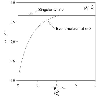
Figure 1: The structure of singularity in the marginally bound (f=0) TBL model for $\rho_{1}\neq 0$ case. Here $\rho_{0}=3$, so the epoch of singularity formation is at $t=t_{0}(0)=2/3$. (a) The event horizon meets the center $r=0$ below the singularity and no null trajectories escape to infinity. The singularity is only locally naked.(b) Singularity is globally naked. There is a family of null geodesics from the singularity which meet the boundary of cloud with $R_{c}>F_{c}$. (c) Graph showing transition from local nakedness to global nakedness, by varying $\rho_{1}$.

5.1 TBL model

Using the local nakedness conditions on the initial data as discussed in the earlier section, we analyze here the global behaviour of RNGs in the TBL model.

5.1.1 $F_{1}\neq 0$

In this case, the singularity is always locally naked, and we have a family of null geodesics coming out of the singularity with apparent horizon as the tangent at the singularity. We see in this case that the singularity can be locally or globally naked (Fig. 1(a), 1(b)). This basically depends upon the chosen value of $\rho_{1}$, and where we place the boundary of the cloud. When the singularity is globally naked, all the RNGs which meet the boundary of the cloud with $R<R_{crit}$ start from the singularity, and the other null geodesics start from the regular center $r=0$ before the singularity is formed.

If we match the density smoothly to zero at the boundary, then $r_{c}=-3F_{0}/4F_{1}=-\rho_{0}/\rho_{1}$, and we see that for $F_{1}<-1.12$ i.e. $\rho_{1}<-4.48$ the singularity is globally naked. In this case the event horizon starts at the singularity $r=0,~{}~{}t=2/3$ as shown in Fig. 1(c). It is seen that for the other case the event horizon formation starts before the epoch of formation of the singularity. It is thus seen that as we depart away from the homogeneous density distribution (the Oppenheimer- Snyder case), by introducing a small density perturbation by choosing a small nonzero value of $\rho_{1}$, the singularity becomes naked. However, it will be only locally naked to begin with and no rays will go outside the event horizon, thus preserving the asymptotic predictability. It follows that even though the strong version of cosmic censorship is violated, the weak censorship is preserved. It is only when the density perturbation is large enough (Fig. 1(c)), beyond a certain critical value, then the singularity will become globally naked, thus becoming visible to the outside observers faraway in the spacetime.

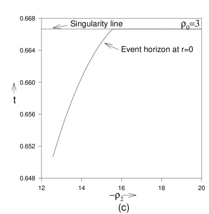
Figure 2: The structure of singularity in marginally bound (f=0) TBL model for $F_{2}\neq 0$, i.e $\rho_{2}\neq 0$ case. We have $\rho_{0}=3$, and $t_{0}(0)=2/3$. (a) Singularity is only locally naked. (b) Singularity is globally naked. There is a family of geodesics from the singularity which meets the boundary of the cloud with $R_{c}>F_{c}$. (c) The graph showing a transition from the locally naked to globally naked singularity by varying $\rho_{2}$.

5.1.2 $F_{2}\neq 0$

The overall behavior in this case (Fig. 2(a), 2(b)) is very similar to $F_{1}\neq 0$ case discussed above. The singularity is always locally naked whenever $F_{2}$ is nonzero, and there is a family of RNGs coming out of singularity with apparent horizon as the tangent. If we match the density smoothly to zero at the boundary of the cloud, then $r_{c}=\sqrt{-3F_{0}/5F_{2}}=\sqrt{-\rho_{0}/\rho_{2}}$. We see that for $F_{2}<-3.1$, i.e. $\rho_{2}<-15.5$, the singularity is always globally naked, while in the other cases it is not globally naked (fig. 2c).

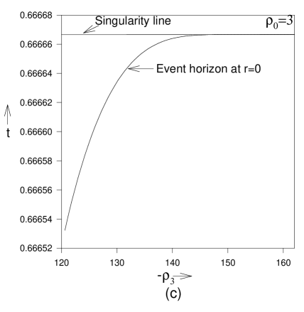
Figure 3: Naked singularity in marginally bound (f=0) TBL model for $F_{3}\neq 0$, i.e. $\rho_{3}\neq 0$ case. (a) Singularity is only locally naked. (b) Singularity is globally naked. There is a family of geodesics from the singularity which meets the boundary of the cloud with $R_{c}>F_{c}$. (c) The graph showing transition from globally naked singularity to a black hole by varying $\rho_{3}$.

5.1.3 $F_{3}\neq 0$

This is the case when the first two derivatives of the density, $\rho_{1}$ and $\rho_{2}$ vanish but $\rho_{3}\neq 0$. In this case $\alpha=3$, and we have two real positive roots for the equation $V(X)=0$ if $\xi={F_{3}}/{F_{0}}^{5/2}<-25.99038=\xi_{crit}$. The singularity is then locally naked, and we see that it is also globally naked with a family of null geodesics meeting the singularity in the past with $X_{0}$ as the tangent (Fig. 3(b)), where $X_{0}$ is the smaller of the two roots. In the range $-1.5>\xi>\xi_{crit}$, the apparent horizon forms at the time of singularity but the singularity is not even locally naked. Numerically we see that (Fig. 3(c)) in this case the event horizon formation starts before the singularity formation as expected.

5.2 Szekeres models

The spherically symmetric TBL models involve no angular dependence for the physical variables such as densities etc. However, it may be possible to examine the effects of such a dependence by using the Szekeres models, which incorporate a certain mode of departure from the spherical symmetry. Thus, this may be a good test case to examine what is possible when non-sphericities are involved. With such a purpose in mind, we keep the form of the mass function $F$ the same as that for the TBL models discussed above, and as a test case we choose the form of $Q$ as given below,

$$Q=\mathrm{cosh}(ar)\zeta\bar{\zeta}+\frac{1}{4\mathrm{cosh}(ar)}.$$

The constant $a$ is chosen in such a way that all regularity conditions are satisfied. Again, we consider the subcases corresponding to different density distributions, as considered earlier.

5.2.1 $F_{1}\neq 0$

The singularity is always locally naked and there is a family of RNGs with $R=F$ near the singularity. We choose a= 1.0. The general behavior of RNGs is similar to that of the similar case in TBL model. But there is a new feature emerging now, which is that the global visibility of singularity in some critical regions can depend upon the value of $\zeta\bar{\zeta}$. That is, the singularity will be globally naked for a certain range of $\zeta\bar{\zeta}$, while for some other range of $\zeta\bar{\zeta}$ it would not be globally naked with the event horizon starting to form before the singularity for these values of $\zeta\bar{\zeta}$ (Fig. 4a).

If we take the boundary of cloud at $r=r_{c}=-3F_{0}/4F_{1}$ then in the range $-1.06<F_{1}<-1.01$, the singularity is globally naked depending on the value of $\zeta\bar{\zeta}$ (Fig. 4a). Therefore the global visibility of singularity is directional. This feature distinguishes singularities in Szekeres spacetimes from TBL model in that the global visibility of the singularity will be related to the directional or angular dependence. For the values $F_{1}<-1.06$, the singularity is globally visible independent of the direction i.e. the values of $\zeta\bar{\zeta}$, whereas for $F_{1}>-1.01$ the singularity is not globally visible for any $\zeta\bar{\zeta}$ values.

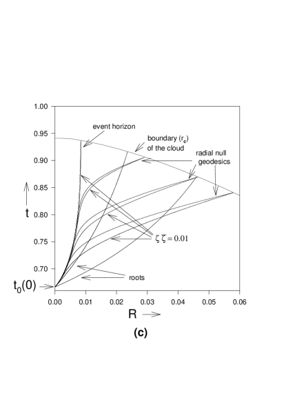
Figure 4: The graph showing the transition from locally naked to globally naked singularity in the marginally bound (f=0) Szekeres quasi-spherical models for different values of $\zeta\bar{\zeta}$. Singularity is located at $t=t_{0}(0)=2/3$. (a) $F_{1}\neq 0$, a = 1.0, boundary of the cloud is at $r_{c}=-3F_{0}/4F_{1}$. (b) $F_{2}\neq 0$, a = 2.0, boundary of the cloud is at $r_{c}=(-3F_{0}/5F_{2})^{1/2}$. (c) The globally naked singularity in the case $F_{3}\neq 0$, a = 3.9.

5.2.2 $F_{2}\neq 0$

The singularity is always locally naked and there is a family of RNGs with tangent as the apparent horizon near the singularity. The general behavior of RNGs is similar to that of $F_{1}$ case above. If we take the boundary of the cloud at $r_{c}=\sqrt{-3F_{0}/5F_{2}}$, then in the range $-3.25<F_{2}<-3.00$ the singularity is globally naked depending on the value of $\zeta\bar{\zeta}$ (Fig. 4(b)). That is, there is a mode of directional global visibility for the singularity. For $F_{2}<-3.25$ the singularity is globally visible independent of the direction, and for $F_{2}>-3.00$ the singularity is not globally visible for any $\zeta\bar{\zeta}$ values.

5.2.3 $F_{3}\neq 0$

In this case $\alpha=3$, and we have two real positive roots for the equation $V(X)=0$ if $\xi={F_{3}}/{F_{0}}^{5/2}<-25.99038=\xi_{crit}$ and the singularity is locally naked. We see in this case that if the singularity is locally naked then it is always globally naked. We can also see numerically that there is a family of geodesics meeting the singularity with $X_{0}$ as the tangent (Fig. 4(c)). But still the equation of trajectories has some dependence on the angle.

6 Conclusions

We have examined here the global visibility and structure of the singularity forming in the gravitational collapse of a dust cloud, in the spherically symmetric TBL case, and also for the aspherical Szekeres models. An interesting feature that emerges, for the marginally bound case, is when we depart from the homogeneous black hole case by introducing a small amount of density perturbation which makes the density distribution inhomogeneous, even though the singularity becomes locally naked the global asymptotic predictability is still preserved. Such a singularity is not globally naked as our numerical results show, till the density perturbation increases and crosses a certain critical value, and thus for small enough density perturbations to the original homogeneous density profile corresponding to the black hole case, the weak cosmic censorship is preserved. This, in a way establishes the stability of the Oppenheimer-Snyder black hole, when the mode of perturbation is that of the density fluctuations in the initial data. It may be noted that this is a different sort of stability as opposed to the stability of the Schwarzschild black hole often referred to in the literature. What we have in mind here is the stability of the formation of black holes in gravitational collapse, involving the inhomogeneities of matter distribution, which remains invariant under small enough density perturbations in the initial density profile from which the collapse evolves.

It remains an interesting question to be examined further as to whether this result will be still intact when we include the nonmarginally bound case, involving the nonzero values of the energy function $f$.

Our analysis also confirms the earlier results [6], deducing in a more specific manner that under physically reasonable initial conditions naked singularities do develop in the Szekeres collapse space-times, which are not spherically symmetric, and admit no Killing vectors. This indicates the possibility that the earlier results for the final fate of spherical gravitational collapse might be valid when suitable generalizations to nonspherical spacetimes are made.

As we have shown here, for the marginally bound TBL and Szekeres models, the global visibility of the singularity is related to the initial data. We classified the range of initial data for expandable mass functions $F(r)$. We see that if the density decreases “fast enough”, that is, when there is sufficient inhomogeneity, then the singularity is globally naked. In the Szekeres models, for some critical range of initial data we see that the singularity is globally naked only for a certain range of $\zeta\bar{\zeta}$. Hence the singularity will be globally visible only in some directions. But there is no such directional dependence as far as the local visibility of the singularity is concerned. Thus our results point out and analyze the global nakedness of the singularity for the collapse of a dust cloud which is either spherical or quasi-spherical, with a regular initial data defined on a regular initial slice.

References

- [1] Penrose R. (1982) , Seminar on Differential Geometry, 631, Princeton University Press, Edited S. T. Yau.
- [2] Szekeres P. (1975) comm. math. Phys. ,55; (1975) Phys. Rev. D , 2941.
- [3] Cooperstock F., Jhingan S., Joshi P. S. and Singh T.P., (1997) Class. Quantum Grav. , 2195.
- [4] Shapiro S. L. and Teukolsky S. A. (1991) American Scientist, 79, 330; (1991) Phys. Rev. Lett. 66, 994; (1992) 13th Int. Conf. on General Relativity and Gravitation, Cordoba, Argentina. and references therein.
- [5] R.C. Tolman (1934) Proc. Natl. Acad. Sci. USA , 410; H. Bondi (1947) Mon. Not. Astron. Soc. , 343.
- [6] Joshi P. S. and Królak A. (1996) Class. Quantum Grav. , 3069.
- [7] Hawking S. W. and Ellis G. F. R. (1973) Large scale structure of space and time. Cambridge University Press.
- [8] P.S. Joshi and I.H. Dwivedi (1993) Phys. Rev. D , 5357.
- [9] S. Jhingan and P. S. Joshi (1998) Annals of the Israel Physical Society Vol. 13, 357.
- [10] T.P. Singh and P. S. Joshi (1996) Class. Quantum Grav. , 559.
- [11] P.S. Joshi and T.P. Singh (1995) Phys. Rev. D51, 677
- [12] W.B. Bonnor (1976) Comm. math. Phys. ,191.