A numerical simulation of pre-big bang cosmology

Abstract

We analyse numerically the onset of pre-big bang inflation in an inhomogeneous, spherically symmetric Universe. Adding a small dilatonic perturbation to a trivial (Milne) background, we find that suitable regions of space undergo dilaton-driven inflation and quickly become spatially flat ($\Omega\rightarrow 1$). Numerical calculations are pushed close enough to the big bang singularity to allow cross checks against previously proposed analytic asymptotic solutions.

CERN-TH/98-24
January 1998

I INTRODUCTION

Increasing attention has recently been devoted to a possible alternative to the standard inflationary paradigm, the so-called pre-big bang (PBB) scenario [1],[2], [3]. While referring the interested reader to [4] for recent reviews of the subject, we will start by just recalling the essential points needed to put the present work in the correct perspective.

The basic postulate of PBB cosmology is, at first sight, a shocking one: our Universe would have originated from an “anti-big bang” state, which was essentially empty, cold, flat, and decoupled. The claim is that, from such innocent-looking initial conditions, a rich Universe can originate thanks to two distinct mechanisms:

• A classical gravitational instability amplifies tiny initial perturbations, inevitably pushing the Universe towards a singularity in the future (to be later identified with the standard big bang) through a phase of accelerated expansion (inflation) and accelerated growth of the coupling. We refer to this phase as dilaton-driven inflation (DDI).

• Quantum fluctuations are amplified during DDI according to the phenomenon by which perturbations freeze out as their wavelength is stretched beyond the Hubble radius. This is how we are able to produce a hot big bang at the end of DDI.

Obviously, in order for the whole scenario to be viable, a mechanism has to be conceived to produce the exit from the dilaton-driven phase to the radiation-dominated phase of standard cosmology. This is the so-called exit problem [5], on which we will have nothing new to say in this paper. Rather, our attention will be focused on the pre-big bang classical epoch, characterized by small couplings and small curvatures (in string units). The big simplification that occurs in this epoch is that the field equations are basically known since they follow from the low-energy tree-level effective action of string theory.

One would like to discuss the most general solution to the field equations and check under which conditions PBB inflation takes place and is sufficiently efficient to produce something like the patch of the Universe presently observable to us. There have been claims [6] that this calls for highly fine–tuned initial conditions. On the other hand, arguments given in [7], [8] have suggested the following interesting possibility/conjecture: the generic initial Universe that is able to give dilaton–driven inflation is one which, in the asymptotic past, converges to the Milne metric with a constant dilaton. Such an initial state does not look generic at first: it is so, however, in a technical sense, i.e. in that the general solution that develops PBB inflation is claimed to depend on as many arbitrary functions of space as the most general solution does. If confirmed, this would mean that PBB inflation covers a non-vanishing fraction of the total phase space (the space of all classical solutions) of string theory.

The main purpose of this paper is to provide a non–trivial check of the above conjecture. We shall not address the full inhomogeneous problem, for the moment, which would require a much stronger numerical effort; we will limit our attention, instead, to the case of a spherically symmetric Universe. We thus consider the problem of how a small spherically symmetric lump (alternatively a shell) of energy affects the otherwise trivial evolution of Milne’s metric. We mention that other interesting questions in spherically symmetric pre-big bang cosmology have been recently addressed by Barrow and Kunze [9].

In Section 2 we define our choice of gauge for the metric and write down the field equations. As usual these break up in two sets: constraints, containing only first time-derivatives, and (constraint-preserving) evolution equations. Luckily, we are able to solve the constraints in closed form and to reduce the equations to four first-order partial differential equations (PDEs) in one time and one space. In Section 3 we apply the general gradient expansion method [10] to our particular case and construct analytic asymptotic solutions near the singularity. In Section 4 we outline our technique for numerically solving the equations and discuss some subtleties needed to avoid possible singularities at $r=0$. The numerical results, both for a spherical lump and for a shell, are reported in Section 5, where comparison and matching with the analytic asymptotic formulae derived in Section 3 are also made. Finally, in Section 6, we interpret our results in the string frame and discuss the relevance of our work to the fine-tuning question raised in [6].

II Field equations and elimination of the constraints

In this paper we shall limit our attention to the graviton–dilaton system in four space–time dimensions. Other fields, such as the axion and various moduli, are taken to be frozen. The low-energy tree-level effective action in the physical (string) frame (whose metric is denoted by $G$) reads [11], [12]:

$$\hbar^{-1}~{}S_{\rm eff}={1\over 2~{}\lambda_{s}^{2}}~{}\int d^{4}x\,\sqrt{-G}\,e^{-\phi}\,\left(R(G)+G^{\mu\nu}\,\partial_{\mu}\phi\,\partial_{\nu}\phi\right)$$ (1)

where $\lambda_{s}$, the string-length parameter, will play no role in the classical regime discussed here. We shall come back to its role in the later evolution in Section 6. The Einstein frame, which turns out to be somewhat more convenient for solving the equations, is related to the string frame by $8\pi G_{\mu\nu}=e^{\phi-\phi_{0}}g_{\mu\nu}$, with $\phi_{0}$ denoting the present value of the dilaton. In that frame, defining $8\pi l_{P}^{2}=\rm{exp}(\phi_{0})\lambda_{s}^{2}$, the action becomes [12]:

$$\hbar^{-1}~{}S_{\rm eff}={1\over 16\pi l_{P}^{2}}\int d^{4}x\sqrt{-g}\left(R(g)-\hbox{1000$\frac{1}{2}$}g^{\mu\nu}\,\partial_{\mu}\phi\,\partial_{\nu}\phi\right)$$ (2)

and leads to Einstein’s equation (after eliminating its trace):

$$R_{\mu\nu}=\hbox{1000$\frac{1}{2}$}\partial_{\mu}\phi\,\partial_{\nu}\phi$$ (3)

and to the dilaton evolution equation:

$$\partial_{\mu}(\sqrt{-g}g^{\mu\nu}\partial_{\nu}\phi)=0\;.$$ (4)

For spherically symmetric cosmological solutions, $\phi$ depends just on time $t$ and on a radial coordinate $\xi$. In the synchronous gauge we can use spatial coordinates such that the metric takes the form (see e.g. [13]):

$$ds^{2}=-dt^{2}+e^{2\alpha(\xi,t)}\,d\xi^{2}+e^{2\beta(\xi,t)}\,d\omega^{2}\;.$$ (5)

where $d\omega^{2}=d\theta^{2}+\sin^{2}\theta\,d\varphi^{2}$. Let us denote by a dot (a prime) differentiation with respect to $t$ ($\xi$), introduce

$$\dot{g}/g\equiv\chi=2\dot{\alpha}+4\dot{\beta}~{},~{}\Delta=2\left(\dot{\alpha}-\dot{\beta}\right)\;,$$ (6)

and recall the expression for the three-curvature ${}^{(3)}R$ on a constant $t$ hypersurface

$${}^{(3)}R=2e^{-2\beta}-2e^{-2\alpha}\left(2\beta^{\prime\prime}+3\beta^{\prime 2}-2\alpha^{\prime}\beta^{\prime}\right)\;.$$ (7)

In terms of these, the full set of field equations consists of

i) the Hamiltonian and momentum constraints:

$$\hbox{1000$\frac{1}{3}$}(\chi^{2}-\Delta^{2})+2~{}{{}^{(3)}R} = {\dot{\phi}}^{2}+e^{-2\alpha}\,\phi^{\prime 2}$$ (8)

$$2\beta^{\prime}\Delta-\hbox{1000$\frac{2}{3}$}(\chi-\Delta)^{\prime} = {\phi}^{\prime}\dot{\phi}\;,$$ (9)

ii) the evolution equations for the metric

$${\dot{\chi}} = -\hbox{1000$\frac{1}{6}$}\left(\chi^{2}+2\Delta^{2}\right)-{\dot{\phi}}^{2}$$ (10)

$$\dot{\Delta}+\hbox{1000$\frac{1}{2}$}\chi\Delta = e^{-2\alpha}\,\phi^{\prime 2}+2e^{-2\beta}+2e^{-2\alpha}\left(\beta^{\prime\prime}-\alpha^{\prime}\beta^{\prime}\right)\;,$$ (11)

and, finally,

iii) the equation for the dilaton

$$\ddot{\phi}+\hbox{1000$\frac{1}{2}$}\chi\dot{\phi}=e^{-2\alpha}\left({\phi}^{\prime\prime}+(2\beta^{\prime}-\alpha^{\prime}){\phi}^{\prime}\right)\;.$$ (12)

This last equation can be shown to be a consequence of the previous ones and we shall therefore ignore it. One can also show that the constraints are conserved in time, thanks to the explicit form of the evolution equations. The Hamiltonian constraint can be written in terms of the well-known $\Omega$ parameter (the fraction of critical energy density) as:

$$\Omega\equiv\rho/\rho_{cr}=3\,{\dot{\phi}^{2}+e^{-2\alpha}\,\phi^{\prime 2}\over\chi^{2}-\Delta^{2}}=1+6\,{{{}^{(3)}R}\over\chi^{2}-\Delta^{2}}\;.$$ (13)

A nice simplification, which occurs in the spherically symmetric case, is that the constraints (9) can be solved explicitly in terms of $\dot{\phi}$ and $\phi^{\prime}$. Given the quadratic character of the constraints, this leads to a four-fold ambiguity, reminiscent of the two-fold ambiguity of the homogeneous case, which we resolve by imposing (in accordance with the PBB postulate) a monotonic behaviour for $\phi$ at least from some time on. We then get:

$$\dot{\phi} = \sqrt{A^{2}+B}+\sqrt{A^{2}-B}\geq 0$$ (14)

$$\phi^{\prime} = e^{\alpha}\left(\sqrt{A^{2}+B}-\sqrt{A^{2}-B}\right)\;,$$ (15)

where the auxiliary quantities $A$ and $B$ are given by

$$A^{2} = \hbox{1000$\frac{1}{12}$}(\chi^{2}-\Delta^{2})+e^{-2\beta}-e^{-2\alpha}(2\beta^{\prime\prime}+3\beta^{\prime 2}-2\alpha^{\prime}\beta^{\prime})$$ (16)

$$B = e^{-\alpha}(\beta^{\prime}\Delta-\hbox{1000$\frac{1}{3}$}(\chi-\Delta)^{\prime})\;.$$ (17)

In conclusion, the final system of evolution equations contains only the metric and can be written in first-order form as:

$${\dot{\alpha}} = \hbox{1000$\frac{1}{6}$}\left(\chi+2\Delta\right)$$ (18)

$${\dot{\beta}} = \hbox{1000$\frac{1}{6}$}\left(\chi-\Delta\right)$$ (19)

$${\dot{\chi}} = -\hbox{1000$\frac{1}{6}$}\chi^{2}-\hbox{1000$\frac{1}{3}$}\Delta^{2}-2(A^{2}+\sqrt{A^{4}-B^{2}})$$ (20)

$${\dot{\Delta}} = -\hbox{1000$\frac{1}{2}$}\chi\Delta+2\,e^{-2\beta}+2\,e^{-2\alpha}(\beta^{\prime\prime}-\alpha^{\prime}\beta^{\prime})+2(A^{2}-\sqrt{A^{4}-B^{2}})\;,$$ (21)

with $A,B$ given in Eq. (17). By using the above relations and the expressions for $\dot{\phi}$ and $\phi^{\prime}$ given in Eq. (15), it is explicitly checked that the “integrability condition” $(\dot{\phi})^{\prime}=(\phi^{\prime})^{\bf.}$ holds.

An essentially trivial solution to all equations is given by the so-called Milne metric, known in the literature [14] because it represents the very late time behaviour (with $\Omega\rightarrow 0$) of all subcritical Universes (with $\Omega<1$). In our gauge, Milne’s metric corresponds to:

$$\alpha=\ln(\pm t)\;,\;\beta=\alpha+\ln\sinh\xi\;,\;\phi=\rm{constant}\;.$$ (22)

It is well known that Milne’s metric can be brought to Minkowski’s form through a coordinate transformation that maps the whole of Milne’s space-time into the (interior of the) forward or backward light cone (depending on the sign of $t$) of Minkowski space-time. The conjecture advanced in [8] is that pre-big bang inflation finds its generic origin in open cosmologies that approach Milne as $t\rightarrow-\infty$. This is why we will choose initial data (at some finite negative $t$) very close to Milne’s Universe, by inserting some lump of energy/momentum through a non-trivial dilaton.

Generic initial data in the spherically symmetric case are known [15] to depend on two arbitrary functions of the radial coordinate $\xi$. It is instructive to see how these two arbitrary functions appear in our initial data. Apparently, in order to select a definite solution to Eqs. (21), one has to provide four functions of $\xi$ on a Cauchy hypersurface, i.e. $\alpha,\beta,\chi$, and $\Delta$ at some initial time. However, two of these can be eliminated by the two residual gauge transformations [15] that keep us inside the synchronous gauge. We may thus take physically distinct initial data to be given by $A$ and $B$ of Eq. (17). Appropriate combinations of $A$ and $B$ represent the initial energy and pressure density of (dilatonic) matter. Equivalently, we may observe that the general spherically symmetric solution of the dilaton evolution equation Eq. (12) is given (in the case of Milne’s metric) by [16]

$$\phi={e^{\tau}\over\sinh\xi}~{}\int_{-\infty}^{\infty}dp~{}b_{p}~{}e^{ip\tau}\left({\sin p\xi\over p}\right)~{}+~{}\rm{constant}\;,~{}\tau\equiv-\ln(-t/T_{0})$$ (23)

and thus depends on two real functions of $p$ (since $b_{p}$ is complex).

This latter observation allows us to make a more general remark: string vacua are usually identified with two-dimensional conformal field theories (CFTs) resulting from a set of $\beta$-function equations [11], [12]. However, within a particular CFT, we can construct marginal (i.e. $(1,1)$) vertex operators representing physical excitations (particles) propagating in the given background. A physical dilaton vertex operator depends upon two (real) functions of space, while a physical graviton vertex depends on four. It is tempting to identify these two (resp. six) degrees of freedom with the classical moduli of our spherically symmetric (resp. generic) solutions, since we can indeed expect a correspondence between marginal operators and the structure of moduli space in the neighborhood of a CFT.

In giving initial data, two precautions have to be taken: i) we should verify that, at least initially, $A^{2}>|B|$, so that all the square roots appearing in Eqs. (21) are real. Consistency requires that this constraint be maintained through the evolution; ii) there is an apparent singularity at $\xi=0$ in $\beta_{Milne}$ and in its derivatives. Of course the singularity is perfectly canceled for Milne’s metric in all equations, but one may encounter numerical problems –or even genuine physical ones– if one is not careful about the way to perturb Milne. We believe that the correct way to avoid curvature singularities and to achieve a smooth algorithm is to insist on an ansatz of the form:

$$\alpha=\alpha(\xi^{2},t)\;,\;\beta=\alpha+\ln\sinh\xi+\xi^{2}\delta(\xi^{2},t)\;,$$ (24)

giving

$$\chi=6~{}\dot{\alpha}+4~{}\xi^{2}\dot{\delta}\;,\;\tilde{\Delta}\equiv\xi^{-2}\Delta=-2\dot{\delta}\;.$$ (25)

It can be checked that, rewriting all equations in terms of $\alpha,\delta,\chi,\tilde{\Delta}$, and their derivatives with respect to $\xi^{2}$, all singularities at $\xi=0$ are automatically removed and that the structure of the ansatz is maintained during the evolution. A possible way to construct sets of “good” initial data along these lines is discussed in the appendix.

III Analytic asymptotic solutions near the singularity

In this section we use, as in [7],[8], the gradient expansion technique [10] to construct analytic asymptotic solutions to our spherically symmetric field equations. This exercise is important in several respects. Firstly, it illustrates the gradient expansion technique in a situation where the momentum constraints can be explicitly solved. Secondly, it will allow a very non-trivial check of the numerical method. Finally, it allows the numerical solutions to be continued in a region where the computation undergoes a critical slowdown because of the singularity. Hence, in the problem at hand, analytic and numerical methods very nicely complement each other.

Assuming that spatial gradients become subleading near the singularity,we can simplify Eqs. (9), (11) to the following form:

$$\dot{\phi}^{2}=\hbox{1000$\frac{1}{3}$}(\chi^{2}-\Delta^{2})~{}~{}~{} ~{}~{}~{}{\phi}^{\prime}=\left(2\beta^{\prime}\Delta-\hbox{1000$\frac{2}{3}$}(\chi-\Delta)^{\prime}\right)\big{/}\dot{\phi}\;,$$ , (26)

$$\dot{\chi}+\hbox{1000$\frac{1}{2}$}\chi^{2}=0~{}~{}~{} ~{}~{}~{}\dot{\Delta}+\hbox{1000$\frac{1}{2}$}\chi\Delta=0\;.$$ , (27)

Following the procedure of Refs. [7], [8] we first solve the evolution equations and obtain:

$$\chi={2\over t-t_{0}(\xi)}\;,\;\Delta={2\lambda(\xi)\over t-t_{0}(\xi)}\;.$$ (28)

The Hamiltonian constraint can be easily solved. Choosing the branch corresponding to a growing dilaton we obtain:

$$\phi(\xi,t)=\phi_{0}(\xi)-{2\over\sqrt{3}}\sqrt{1-\lambda^{2}}\ln\left({t/t_{0}(\xi)}-1\right)\;,\;t<t_{0}\;.$$ (29)

We now integrate once more the evolution equations to obtain the metric:

$$\alpha = \gamma(\xi)+\hbox{1000$\frac{1}{3}$}\left(1+2\lambda(\xi)\right)\,\ln\left({t/t_{0}(\xi)}-1\right)\;,$$ (30)

$$\beta = \delta(\xi)+\hbox{1000$\frac{1}{3}$}\left(1-\lambda(\xi)\right)\,\ln\left({t/t_{0}(\xi)}-1\right)\;.$$ (31)

Finally, we solve the momentum constraint. Most terms automatically match and we get the single condition:

$$\phi_{0}^{\prime}=-{2\sqrt{3}\over\sqrt{1-\lambda^{2}}}\left(\lambda^{\prime}/3+\lambda\delta^{\prime}\right)\;.$$ (32)

The general solution thus appears to depend upon four functions of space, i.e. $\lambda,\gamma,\delta$, and $t_{0}$, giving the line-element:

$$ds^{2}=-dt^{2}+\left(t/t_{0}-1\right)^{2/3(1-\lambda)}\left[\left(t/t_{0}-1\right)^{2\lambda}\,e^{2\gamma}\,d\xi^{2}+\,e^{2\delta}d\omega^{2}\right]$$ (33)

Obviously, we can reabsorb $\gamma$ in a redefinition of the $\xi$ coordinate, $dr=e^{\gamma}d\xi$. Similarly, the choice of equal-time slices allows us to remove the space dependence of $t_{0}$. We are thus left, as in the previous section, with just two physically meaningful functions of $\xi$ for the characterization of our dynamical system, as should be the case for the general spherically symmetric solution [15].

Actually, the situation is a bit more subtle as far as the $\xi$ dependence of $t_{0}$ is concerned. Inserting the above asymptotic solution back into the exact equations, one finds that spatial derivatives are only subleading for sufficiently small values of $t_{0}^{\prime}(\xi)$. In other words, at least in the Einstein frame, one has to choose appropriate time slices so that $t_{0}$ is constant and only then can one neglect spatial derivatives. Constructing these privileged time slices is not a simple problem and therefore, in this paper, we will only check (see Section 5) the asymptotic formulae in the vicinity of the minimum of $t_{0}$ (i.e. near the point where the singularity is first reached). In Section 6 we will argue that an alternative solution to this problem consists in going over to the synchronous gauge in the string frame. In this case, spatial derivatives (at fixed string-frame time) turn out to be always subleading near the singularity. This suggests that it would be desirable to numerically solve the equations directly in the string frame.

IV The numerical approach

We shall now briefly describe the essential aspects of the numerical algorithm and its practical implementation. The system given by Eqs. (21) is similar to a Hamiltonian one with an infinite number of degrees of freedom. Its numerical implementation must necessarily introduce a limit on the number of degrees of freedom, which can be done in several ways. Our present choice is to introduce a finite grid in the variable $\xi$ and to define the derivatives with respect to $\xi$ by a spectral method, based on the Fourier transform, which allows us to reach a high precision. Alternative techniques, such as using a symbolic language or applying finite elements techniques, will be considered in the near future. In our approach, a special care must be devoted to boundary conditions, since the Fourier transform preferably works in periodic boundary conditions, which are not adequate to our problem. As we explain later on, this problem is solved by letting $\xi$ extend to a symmetric interval and by continuing the fields to the negative $\xi$-axis. Time evolution is generated via a standard integration routine with variable step and local error control.

To prepare the equations to be implemented in numerical terms, it is convenient to introduce new fields, which describe the metric as a perturbation from a Milne background:

$$\alpha_{s} = \alpha+\tau$$ (34)

$$\beta_{s} = \beta+\tau-\ln\sinh\xi$$ (35)

$$\chi_{s} = e^{-\tau}\,\chi$$ (36)

$$\Delta_{s} = e^{-\tau}\,\Delta$$ (37)

where $\tau$ is defined by $t=-\exp(-\tau)$. The advantage of working in the Milne background is that the shifted fields, unlike the background, vanish at $\xi=\infty$ and we can thus introduce a finite volume cutoff. The boundary conditions at $\xi=0$ are crucial; as we have already noticed, regularity at $\xi=0$ is achieved if we assume Eq. (24), in the equivalent form

$$\beta_{s}(\xi,\tau) = \alpha_{s}(\xi,\tau)+\xi\,\eta(\xi,\tau)$$ (38)

$$\Delta_{s}(\xi,\tau) = \xi\,\Sigma(\xi,\tau)$$ (39)

with boundary conditions at $\xi=0$

$$\eta(0,\tau) = \Sigma(0,\tau)=0\,,$$ (40)

$$\alpha_{s}(0,\tau)^{\prime} = \chi_{s}(0,\tau)^{\prime}=0\;.$$ (41)

In order to satisfy these boundary conditions and still apply the Fourier transform to compute field derivatives, we continue the fields to a symmetric interval $-L<\xi<+L$; we enforce the correct boundary conditions by extending $\alpha_{s},\chi_{s}$ to symmetric functions and $\eta,\Sigma$ to antisymmetric ones. In terms of the new fields, the system (21) becomes

$${d\alpha_{s}\over d\tau} = \hbox{1000$\frac{1}{6}$}(\chi_{s}+6+2\,\xi\Sigma)$$ (42)

$${d\eta\over d\tau} = -\hbox{1000$\frac{1}{2}$}\Sigma$$ (43)

$${d\chi_{s}\over d\tau} = -\chi_{s}-\hbox{1000$\frac{1}{6}$}\chi_{s}^{2}-\hbox{1000$\frac{1}{3}$}\Delta_{s}^{2}-\Lambda_{+}$$ (44)

$${d\Sigma\over d\tau} = -\Sigma-\hbox{1000$\frac{1}{2}$}\chi_{s}\Sigma+2\,\xi^{-1}\,e^{-2\alpha_{s}}\,\left({e^{-2\xi\eta}-1\over\sinh^{2}\xi}+\beta_{s}^{\prime\prime}-\alpha_{s}^{\prime}\,(\beta_{s}^{\prime}+\coth\xi)\right)+\xi^{-1}\,\Lambda_{-},$$ (45)

where

$$\Lambda_{\pm} = 2\,\left(A_{s}^{2}\pm\sqrt{A_{s}^{4}-B_{s}^{2}}\right)$$ (46)

$$A_{s}^{2} = \hbox{1000$\frac{1}{12}$}\left(\chi_{s}^{2}-\Delta_{s}^{2}\right)+$$ (48)

$$e^{-2\alpha_{s}}\left({e^{-2\xi\eta_{s}}-1\over\sinh^{2}\xi}-3-2\beta_{s}^{\prime\prime}-3\beta_{s}^{{}^{\prime}2}-2(3\beta_{s}^{\prime}-\alpha_{s}^{\prime})\,\coth\xi+2\alpha_{s}^{\prime}\beta_{s}^{\prime}\right)$$

$$B_{s} = e^{-\alpha_{s}}\,\left(\Delta_{s}\,(\beta_{s}^{\prime}+\coth\xi)-\hbox{1000$\frac{1}{3}$}(\chi_{s}^{\prime}-\Delta_{s}^{\prime})\right)\;.$$ (49)

and Eq. (39) is understood.

Notice that the system is identically satisfied by taking $\alpha_{s}=\eta=\Sigma=0$ and $\chi_{s}=-6$, which represents Milne’s background. The initial conditions we want to examine are given by Eq. (A2) (with $\zeta=0$), which in terms of the shifted fields reads as follows:

$$\alpha_{s}(\xi,0) = \hbox{1000$\frac{1}{4}$}\ln\left(1-{\mu\over\cosh[\varepsilon(\xi-\xi_{0})]}\right)\,+\,(\xi_{0}\longrightarrow-\xi_{0})$$ (50)

$$\chi_{s}(\xi,0) = -6\,\exp\{-2\alpha_{s}(\xi,0)\}$$ (51)

$$\eta(\xi,0) = \Sigma(\xi,0)=0,$$ (52)

where $\mu$ is a suitable constant. We have implemented this system of partial differential equations in matlab${}^{\cite[cite]{[\@@bibref{Number}{mat}{}{}]}}$, which offers very efficient built-in routines for integrating ordinary differential equations, a fast Fourier transform and an integrated graphic environment. The only tricky point in the numerical treatment of these equations refers to the delicate cancelation mechanism that makes the solutions regular at $\xi=0$ in spite of the apparent singular nature of the terms involving $\coth\xi$ and $\sinh^{-2}\xi$. This cancelation, which takes place in exact arithmetic, is spoiled by finite precision arithmetic and makes the solution singular after a short time evolution. The remedy that we adopt consists in enforcing regularity near the origin by a polynomial interpolation and a Fourier filtering, which truncates high frequency components above a certain cutoff. A consistency check is given by solving the equations with various initial ansatze corresponding to $\xi_{0}=0$ or $\xi_{0}>0$. The former case represents a spherically symmetric perturbation concentrated at the origin, while the latter spreads out over a spherical shell and naturally avoids the singularity. A similar behaviour is indeed observed in both cases with fields $\alpha$ and $\chi$ blowing up as $\Omega$ approaches 1.

V Numerical results

We report some preliminary results obtained by running our code with the initial ansatz given by Eq. (51) and for several values of the parameters ($\xi_{0},\varepsilon,\mu$); a typical run involves a grid with $N=4096$ points and takes less than an hour on a modern workstation. We set a finite-size $L\approx 10/\varepsilon+\xi_{0}$ and an ultraviolet cutoff at half way to the size of the Brillouin zone. The routine ode45 of matlab can be used with its standard setup; a special care must be devoted to the choice of the absolute tolerance parameter which should be set differently for the various fields which have very different scales. The evolution starts at negative $t$ from the ansatz of Eq. (51); we report both cases ($\xi_{0}=0$ and $\xi_{0}>0$), which indeed show a similar pattern (see Figs.(1,3)). In Figs.(2,4) both $\Omega$ and the dilaton are shown.

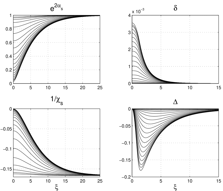
FIG. 1.: The fields $\alpha_{s},\chi_{s},\eta,\Delta_{s}$ starting with $\xi_{0}=0,\mu=0.01,\varepsilon=.2$.

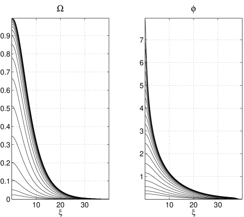
FIG. 2.: The $\Omega$ parameter and the dilaton, same initial data as above.

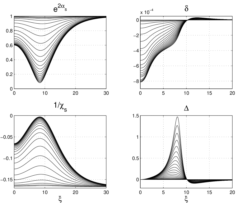
FIG. 3.: The fields $\alpha_{s},\chi_{s},\eta,\Delta_{s}$ starting with $\xi_{0}=10,\mu=0.01,\varepsilon=0.2$.

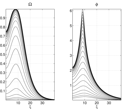
FIG. 4.: The $\Omega$ parameter and the dilaton, same initial data as above.

We examined the numerical solution in order to check the validity of the approximation introduced in Sec.III. In particular we were able to check the asymptotic behaviour in the region where $\Omega$ is very close to 1, where Eqs. (28) and (31) predict a linear regime in time for the following expressions

$$W_{1} = 1/\chi$$ (53)

$$W_{2} = \exp\{\alpha+2\beta\}$$ (54)

$$W_{3} = \exp\{-(\hbox{1000$\frac{3}{2}$}\phi+\alpha+2\beta)/(\surd 3-1)\}$$ (55)

(notice that the value of $\lambda$ is negligible). This is clearly displayed in Fig.5.

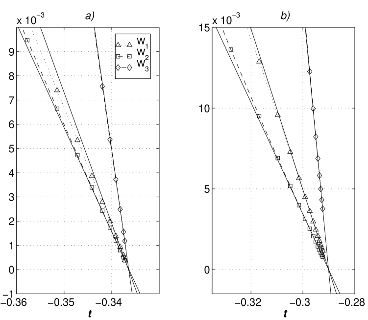
FIG. 5.: The asymptotic behaviour ${\cal O}(t_{0}(\xi)-t)$ for the variables $W_{n}$ at the $\Omega$ peak (a) $\xi_{0}=0$, b) $\xi_{0}=10$)

From a linear fit to the data, it is then possible to extract information about the unknown functions $t_{0}(\xi)$ and $\lambda(\xi)$. We find that, as expected, $t_{0}(\xi)$ has an extremum near the $\Omega$ peak with a small curvature $t(\xi)^{\prime\prime}$, which is responsible for the small deviations from the asymptotic estimates of Eq. (28) (see Fig.6).

In all the cases we have examined so far, the function $\lambda(\xi)$ turns out to be very small (see Fig.7). but this is probably due to our initial starting point with $\Delta\equiv 0$. We are currently exploring a wider class of initial data, in order to find the generic properties of the solutions.

.

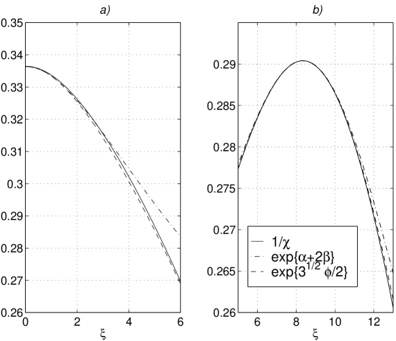
FIG. 6.: The blowing–up time $t_{0}(\xi)$, (a) $\xi_{0}=0$, b) $\xi_{0}=10$)

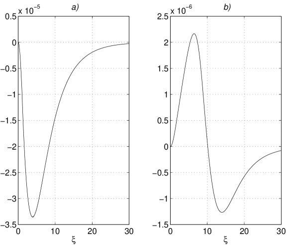
FIG. 7.: The function $\lambda(\xi)$, (a) $\xi_{0}=0$, b) $\xi_{0}=10$).

Finally, our code can also be run backwards i.e. towards $t=-\infty$. In this case, however, we encounter a problem: although $\phi$ keeps decreasing in magnitude as $t$ becomes more and more negative, it also starts to oscillate, as expected [8]. As a result, the constraints cannot be always solved with the sign determination given in (15). We have been able to solve this problem by imposing the constraints only on the initial data and by otherwise working in an enlarged phase space containing also $\phi$ and $\dot{\phi}$. This procedure has the further advantage of allowing a non-trivial check of the numerical precision by verifying that the constraints are conserved.

We expect to present results obtained by following this better procedure in the near future.

VI Discussion

In order to discuss better the physical meaning of our result it would be convenient to transform them back to the original string frame. It is difficult to make the change of frame numerically and, indeed, we think it would be easier to start directly the whole exercise in the new frame. Fortunately, we can achieve a semi-quantitative understanding of the string frame solutions by noticing that:

• initially the two frames coincide, since the dilaton is constant;

• our numerical results, as the singularity is approached, fit very well with the analytic asymptotic formulae given in Section 3.

The latter observation allows us to perform the passage to the string frame analytically (and of course approximately) near the singularity. Following Ref. [7] we find rather easily that the asymptotic metric and dilaton in the string-frame synchronous gauge are given by

$$ds^{2} = -dt^{2}+\left[\left(t/t_{0}-1\right)^{2\alpha_{\xi}}\,e^{2\tilde{\gamma}}\,d\xi^{2}+\left(t/t_{0}-1\right)^{2\alpha_{\theta,\varphi}}\,e^{2\tilde{\delta}}d\omega^{2}\right]~{}~{},$$ (56)

$$\phi(\xi,t) = \phi_{0}(\xi)+{\gamma_{\phi}}\,\ln\left({t/t_{0}(\xi)}-1\right)\;,\;t\rightarrow t_{0}$$ (57)

where, for notational simplicity, we kept denoting by $t$ the string frame time and by $t_{0}(\xi)$ the location of the singularity. The important exponents $\alpha_{i}$ and $\gamma_{\phi}$ are completely determined by the function $\lambda(\xi)$ appearing in Eq. (28). We find:

$$\alpha_{\xi} = -{1\over\sqrt{3}}{2\sqrt{1-\lambda^{2}}-\sqrt{3}\lambda^{2}-2\lambda~{}(\sqrt{3}+\sqrt{1-\lambda^{2}})\over 2+\lambda^{2}}~{}~{},$$ (58)

$$\alpha_{\theta,\varphi} = -{1\over\sqrt{3}}{2\sqrt{1-\lambda^{2}}-\sqrt{3}\lambda^{2}+\lambda~{}(\sqrt{3}+\sqrt{1-\lambda^{2}})\over 2+\lambda^{2}}~{}~{},$$ (59)

$$\gamma_{\phi} = -{2(1-\lambda^{2})+2\sqrt{3}\sqrt{1-\lambda^{2}}\over 2+\lambda^{2}}~{}~{}.$$ (60)

It is reassuring to check that the $\alpha_{i}$ satisfy Kasner’s condition:

$$\sum\alpha_{i}^{2}=\alpha_{\xi}^{2}+2\alpha_{\theta,\varphi}^{2}=1$$ (61)

and that, furthermore,

$$\gamma_{\phi}-\sum\alpha_{i}=-1$$ (62)

as in the homogeneous case. Also note that, in the limit $\lambda\ll 1$, $\alpha_{i}\rightarrow-1/\sqrt{3}$. This corresponds to the isotropic limit. From the above formulae we see that, in the string frame, the metric is typically (super)inflationary since the inequalities $-1<\alpha_{i}<0$ are almost always fulfilled. It is easy to check that, as a consequence, the string frame asymptotic solution is reliable even if one does not choose time slices corresponding to $t_{0}\sim\rm{constant}$. The expansion rate is maximal for the regions where $\lambda$ is very close to zero, i.e. for very isotropic regions.

We conclude that, as anticipated in refs. [7],[8], regions with the correct dilaton perturbation do undergo a superinflationary expansion, become asymptotically flat and, most likely, isotropic. It would of course be most interesting to attempt to generalize our computations to the case of several lumps and/or shells located randomly in space and with random initial parameters and see what kind of chaotic inflationary Universe will result. This, unfortunately, appears to demand going beyond the spherically symmetric situation we have considered in this paper.

In conclusion, our numerical approach appears to confirm that, at least in the case of spherical symmetry, dilaton-driven inflation naturally emerges as a classical gravitational instability of small perturbations around the trivial (Milne) vacuum. Nonetheless, before being able to address/answer completely the criticism expressed in [6], the present work needs to be expanded in at least two directions: i) classical phase space has to be swept more systematically, in particular away from the case of spherical symmetry; ii) the behaviour at very early times has to be thoroughly investigated so that the possibility (see N. Kaloper et al. [6]) that quantum fluctuations at very early times may destroy the homogeneity needed for turning on dilaton-driven inflation is properly assessed. As discussed at the end of Section V, this latter problem requires a new way of enforcing the constraints on which we are presently working and hope to report soon.

A A procedure to generate a class of admissible initial data

In this appendix we illustrate our procedure for choosing the small initial perturbation of Milne’s metric in such a way as to fulfill the necessary positivity constraints as well as regularity at $\xi=0$. The physical idea is quite simple: since we know that Milne’s solution is regular and satisfies all the constraints, we construct initial data from a small deformation of Milne. Notice that there is no need that the deformation satisfies the evolution equations.

Consider the following deformation of Milne’s metric:

$$\alpha = {1\over 4}\ln\left(t^{2}-{{T_{0}^{2}}\over{\cosh{\varepsilon(\xi-\xi_{0})}}}\right)+(\xi\rightarrow-\xi)\;,$$ (A1)

$$\beta = \alpha+\ln~{}\sinh\xi+\hbox{1000$\frac{1}{2}$}\zeta\left[{{T_{0}^{2}\xi^{2}}\over{t^{2}\cosh{\varepsilon(\xi-\xi_{1})}}}+(\xi\rightarrow-\xi)\right]$$ (A2)

Such a deformation is localized at $\xi=\xi_{0}$, with some anisotropy concentrated at $\xi_{1}$. The deformation rapidly drops to zero far from these two values of $\xi$. The symmetrization is needed in order to bring the ansatz in the form discussed ion Section 3. We now define the initial data from Eqs. (A2) and their first time derivatives at the initial time $t_{i}\ll T_{0}$.

We have performed the computation of the initial data using Mathematica and checked that the positivity and regularity constraints are identically satisfied in $\xi$ for a wide choice of the parameters $t_{i}/T_{0},~{}\varepsilon,~{}\xi_{0},~{}\xi_{1},~{}\zeta$, e.g. for the sets used in section 5:

$$t_{i}/T_{0}=10,\;\varepsilon=0.2,\;\xi_{0}=0,\;\zeta=0;$$ (A3)

$$t_{i}/T_{0}=10,\;\varepsilon=0.2,\;\xi_{0}=10,\;\zeta=0\,.$$ (A4)

Indeed, positivity is most sensitive to the parameter $\varepsilon$ which cannot be much larger than $0.5$. In the limit $t_{i}/T_{0}\rightarrow\infty$ the formulae for the initial data simplify considerably and positivity constraints can be solved in many cases analytically.

The above initial choice, that we have considered for our numerical study, is a special case of a class of admissible initial data (we call a given choice of initial data admissible if it satisfies the constraint $A^{2}\geq|B|$) which can be characterised as follows:

theorem:  Let $f(\xi)$ be twice continuously differentiable with

1. $f(\xi)\geq f_{0}>1$;

2. $f^{\prime}(0)=0$;

3. $f^{\prime\prime}(\xi)\leq\varepsilon^{2}\,f(\xi)$ for some $\varepsilon<1$.

Then the initial data given by

$$\alpha_{s}=\hbox{1000$\frac{1}{2}$}\ln(1-f(\xi)^{-1})\,,\;\chi_{s}=-6\,e^{-2\alpha_{s}}\,,\;\eta=\,\Sigma\,=0\;.$$ (A5)

are admissible if

$$f_{0}^{-1}\leq\max[{5-4\,\varepsilon-2\,\varepsilon^{2}\over 6-4\,\varepsilon-2\,\varepsilon^{2}}\,,\,1-({2\,\varepsilon\over 3-2\,\varepsilon-\varepsilon^{2}})^{2}\;]\;.$$ (A6)

We shall first prove the following

lemma: Let $f(\xi)$ satisfy the conditions of the previous theorem. Then

$$-\varepsilon\leq{f^{\prime}(\xi)\over f(\xi)}\leq\varepsilon\tanh\varepsilon\xi$$ (A7)

proof: Let $g=f^{\prime}/f$; then it holds

$${dg(\xi)\over d\xi}\leq\varepsilon^{2}-g(\xi)^{2}\;.$$ (A8)

First of all let us show that if $g(\overline{\xi})<-\varepsilon$ for some $\overline{\xi}$, $g$ would develop a singularity at a finite $\xi$: under the assumption and the previous inequality Eq. (A8) it would follow

$${g^{\prime}(\xi)\over\varepsilon^{2}-g(\xi)^{2}}\geq 1$$ (A9)

which can be integrated to give

$$\int_{g(\xi)}^{g(\overline{\xi})}{dg\over g^{2}-\varepsilon^{2}}\geq\xi-\overline{\xi}\;.$$ (A10)

Since the integral is convergent, $g\to-\infty$ at a finite $\xi$; $f$ being regular and $>1$ this is a contradiction. Assume next that $g(\xi)>\varepsilon\tanh\varepsilon\xi$ at some $\overline{\xi}$; by continuity we may assume $g(\overline{\xi})<\varepsilon$. It follows

$${g^{\prime}(\xi)\over\varepsilon^{2}-g(\xi)^{2}}\leq 1\;;$$ (A11)

by integrating from $\xi=0$ we find $\tanh^{-1}(g(\overline{\xi})/\varepsilon)\leq\varepsilon\overline{\xi}$, a contradiction. This completes the proof of the lemma.

To prove the main theorem, let us insert Eq. (A5) into the expression of $A_{s}^{2}\pm B_{s}$ (Eq. (49)); we get

$$(f-1)\,\exp\{2\alpha_{s}\}\,\left(A_{s}^{2}\pm B_{s}\right) =$$ (A12)

$$3-{f^{\prime\prime}\over f} + {2f-5/4\over f-1}\,\left({f^{\prime}\over f}\right)^{2}-2\,{f^{\prime}\over f}\,\coth\xi\,\pm\,2\,{f^{\prime}\over f}\sqrt{f\over f-1}\;.$$ (A13)

We can apply the lemma at once and see that the l.h.s. is bound from below as follows

$${\rm l.h.s.}\geq 3-\varepsilon^{2}-2\,\varepsilon+2\left({f^{\prime}\over f}\right)^{2}\,\pm\,2\,{f^{\prime}\over f}\,\sqrt{f\over f-1}$$ (A14)

or, we may complete the square before applying the inequality,

$${\rm l.h.s.}\geq 3-\varepsilon^{2}-2\,\varepsilon-\hbox{1000$\frac{1}{2}$}{f\over f-1}+2\left({f^{\prime}\over f}\pm\hbox{1000$\frac{1}{2}$}\sqrt{{f\over f-1}}\right)^{2}$$ (A15)

and the result follows. Notice that the theorem covers the cases that we have considered in section IV; the domain of parameters for which the data are admissible is shown in Fig.8.

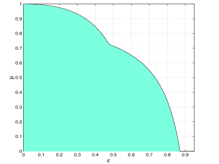
FIG. 8.: Admissible values for $\mu,\varepsilon$.

The class of initial data which has been defined here depends on a single arbitrary function. The general expression of $f$ can be easily derived by setting $\varepsilon^{2}f-f^{\prime\prime}=\rho(\xi)\geq 0$. The solution is clearly

$$f(\xi)=\mu^{-1}\cosh(\varepsilon\xi)-\int_{0}^{\xi}\varepsilon^{-1}\sinh\left(\varepsilon(\xi-\xi^{\prime})\right)\,\rho(\xi^{\prime})\,d\xi^{\prime}\;.$$ (A16)

If $\int_{0}^{\infty}\rho(\xi)\,d\xi\,$ is small enough, then we get admissible initial data. As stressed in Sec.II, it would be interesting to have a general characterisation of suitable Cauchy data.

REFERENCES

- [1] G. Veneziano, Phys. Lett. B265 (1991) 287.
- [2] M. Gasperini and G. Veneziano, Astropart. Phys. 1(1993) 317; Mod. Phys. Lett. A8 (1993) 3701; Phys. Rev. D50 (1994) 2519.
- [3] An updated collection of papers on the PBB scenario is available at http://www.to.infn.it/teorici/gasperini.
- [4] G. Veneziano, Status of String Cosmology: Basic Concepts and Main Consequences, in String Gravity and Physics at the Planck Energy Scale, Erice 95, N. Sanchez and A. Zichichi Eds. (Kluver Academic Publishers, Boston,1996), p. 285; A simple/short introduction to pre–big bang physics/cosmology, in Highlights: 50 years later, Erice 97, hep-th/9802057
-
[5]
M. Gasperini, M. Maggiore and G. Veneziano,
Nucl. Phys. B494 (1997) 315;
R. Brustein and R. Madden, Phys. Lett B410 (1997) 110; Phys. Rev. D57 (1998) 712, and references therein. -
[6]
M. Turner and E. Weinberg, Phys. Rev. D56 (1997) 4604;
see also N. Kaloper, A. Linde and R. Bousso, Pre-Big-Bang Requires the Universe to be Exponentially Large from the Very Beginning, hep-th/9801073. - [7] G. Veneziano, Phys. Lett. B406 (1997) 297.
- [8] A. Buonanno, K. A. Meissner, C. Ungarelli and G. Veneziano, Classical inhomogeneities in string cosmology, hep-th/9706221, Phys. Rev. D, in press.
- [9] J. D. Barrow and K. E. Kunze, Spherical Curvature Inhomogeneities in String Cosmology, hep-th/9710018.
-
[10]
V. A. Belinskii and I. M. Khalatnikov,
Sov. Phys. (JETP) 36 (1973) 591;
N. Deruelle and D. Langlois, Phys. Rev. D52 (1995) 2007;
J. Parry, D. S. Salopek and J. M. Stewart, Phys. Rev. D49 (1994) 2872. - [11] C. Lovelace, Phys. Letters B135 (1984) 75.
-
[12]
E.S. Fradkin and A.A. Tseytlin,
Nucl. Phys. B261 (1985) 1;
C.G. Callan, D. Friedan, E.J. Martinec and M.J. Perry, Nucl. Phys.B262 (1985) 593;
A. Sen, Phys. Rev. D32 (1985) 2102. - [13] S. Weinberg, Gravitation and Cosmology, (John Wiley and Sons, Inc., New York, 1972).
- [14] Ya. B. Zeldovich and I. D. Novikov, Relativistic Astrophysics, Vol. II (Structure and Evolution of the Universe), Section 2.4.
- [15] L. Landau and E. Lifshitz, The Classical Theory of Fields, (Pergamon Press, Oxford, 1962) p. 323.
- [16] T. Tanaka and M. Sasaki, Phys. Rev. D55 (1997) 6061.
- [17] © The Math Works, Inc., Natick, Massachusetts (http://www.mathworks.com).