Self-Organized (Quasi-)Criticality: the Extremal Feder and Feder Model

Abstract

A simple random-neighbor SOC model that combines properties of the Bak-Sneppen and the relaxation oscillators (slip-stick) models is introduced. The analysis in terms of branching processes is transparent and gives insight about the development of large but finite mean avalanche sizes in dissipative models. In the thermodynamic limit, the distribution of states has a simple analytical form and the mean avalanche size, as a function of the coupling parameter strength, is exactly calculable.

PACS number: 05.40.+j, 05.70.Ln, 64.60.Ht, 91.30.Bi.

]

I Introduction

Although self-organized criticality (SOC) is perhaps not the whole story for the emergence of scale invariance in natural systems, certainly it is a promising concept in the understanding of how Nature works [1]. The fact that still there is not a clear picture of the necessary and/or sufficient mechanisms to create the self-organized critical state is reflected in the doubts about whether locally dissipative systems really presents SOC or have only an exponential divergence of the mean avalanche size $\langle s\rangle$ when approaching the conservative limit. The recent result by Chabanol and Hakin [2] and by Brock and Grassberger [3] stating that the random-neighbor OFC model is not critical in the dissipative regime, contradicting a previous claim of Lise and Jansen [4], is a clear example of the difficulty of making that distinction by using only simulation evidence. An instance where this also happened is the forest-fire model [5], which has only a very large mean avalanche size, not an infinite one like in critical systems.

In this paper, a model is proposed which is similar but simpler than the random-neighbor slip-stick model studied in [2, 3]. In this model the distribution of states $p(E)$ and the mean avalanche size $\langle s\rangle$, as functions of a dissipative parameter $\alpha$, have exactly calculable analytical forms (in the infinite system size limit). The analysis in terms of branching processes is transparent and gives a clear mechanism for the emergence of large but finite $\langle s\rangle$ in systems with local dissipation. The concept of quasi-criticality is also discussed as a convenient distinction to be made in the classification of the various systems studied in the SOC literature.

II Extremal Feder and Feder model

A The model

The model is a random-neighbor version of the Feder and Feder model [3, 6] where it is used an extremal dynamics similar to the Bak-Sneppen model [7] instead of the standard global driving. All sites $j=1,\ldots,N$ have a continuous state variable $E_{j}\in{\cal R}$. At each time step the site with maximal value ‘fires’, resetting its value to zero plus a noise term $\eta$. Then, $k$ random ‘neighbors’ ($rn$) of the firing site have their states incremented by a constant $\alpha$ plus a noise term. The choice of neighbors is done at the firing instant: the randomness is annealed. So, denoting the site with maximal value at instant $t$ as $E^{*}_{i}\equiv\mbox{max}\{E_{j}\}$, the update rules are:

$$E_{i}^{*}(t+1) = \eta\>,$$ (1)

$$E_{rn}(t+1) = E_{rn}(t)+\alpha+\eta\>,$$ (2)

with $\eta$ being a random variable uniformly distributed in the interval $[0,\epsilon]$ (the range of $\epsilon$ will be discussed later). Note that each site receives a different quantity $\eta$.

Consider the instantaneous density of states $p(E,t)$. It is clear that for any $E$ outside the intervals $I_{n}\equiv[(n-1)\alpha,(n-1)\alpha+n\epsilon],n=1,2,\ldots$, this density decays to zero for long times. These intervals effectively discretize the phase space, so it is useful to define the following quantities,

$$P_{n}=\int_{(n-1)\alpha}^{(n-1)\alpha+n\epsilon}p(E)dE\>,$$ (3)

with $n=1,2,\ldots,n_{max}$, and $\epsilon<\alpha/n_{max}$ so that the intervals do not overlap (the integer $n_{max}$ will be obtained latter). The process can be thought of as a transference of sites between the intervals $I_{n}$. At each time step, one site is transferred to the interval $I_{1}$ and, with probability $kP_{1}$, one site is removed from this interval. The average flux to the intervals $I_{n}$ with $n>1$ corresponds to the probability $kP_{n-1}$ that a neighbor is chosen in the previous $I_{n-1}$ interval minus the probability $kP_{n}$ that a neighbor is chosen in the interval $I_{n}$. The average number of sites in each interval is $N_{n}(t)=NP_{n}(t)$. For long times, that is, when the density of states outside the $I_{n}$ intervals goes to zero, one can write

$$P_{1}(t+1) = P_{1}(t)+\frac{1}{N}\left[1-kP_{1}(t)\right]\>,$$ (4)

$$P_{n}(t+1) = P_{n}(t)+\frac{1}{N}\left[kP_{n-1}(t)-kP_{n}(t)\right]\>.$$ (5)

Here, each time step is equal to the update of the maximal site and $k$ random neighbors.

The condition for steady states, $P_{n}(t+1)=P_{n}(t)=P_{n}^{*}$, gives

$$P_{1}^{*} = 1/k\>,$$ (6)

$$P_{n}^{*} = P_{n-1}^{*}\>,$$ (7)

that is, $P_{n}^{*}=1/k$ for all $n$. But since $p(E)$ is normalized, only $n_{max}$ intervals with $P_{n}$ of ${\cal O}(1)$ can exist. That is,

$$\sum_{n=1}^{n_{max}}P_{n}^{*}=n_{max}\times\frac{1}{k}=1.$$ (8)

This means that $p(E)$ is composed of $k$ bumps ($n=1,\ldots,n_{max}=k$) and the previous condition for producing non-overlapping intervals $P_{n}$ reads $\epsilon<\alpha/k$. There is also a bump of ${\cal O}(\log N/N)$ (by analogy with the results from [8]) situated at the interval $I_{k+1}=[k\alpha,k\alpha+(k+1)\epsilon]$. The other intervals $n>k+1$ have $P_{n}$ of yet smaller order (see Fig 1).

B Avalanches

An avalanche will be defined as the number of firing sites until an extremal site value falls bellow the threshold $E_{th}=1$. Note that the first site of an avalanche (the ‘seed’) always has $E<1$ but it counts as a firing site. So, if a seed produces no supra-threshold sites (‘descendants’), this counts as an avalanche of size one. This definition of avalanches agree with that used in the studies of relaxation oscillator models.

In these random neighbor models, an avalanche can be identified as a branching process where an active site produces $k$ new sites, each one having a probability $p$ of being active (a ‘branch’) and a probability $1-p$ of being inactive (a ‘leave’). The branching ratio $\sigma=kp$ measures the probability that a firing site produces another firing site. Now, consider an avalanche which has terminated after $s$ sites have fired. This avalanche is composed by one seed and $s-1$ descendants. But the average number of descendants produced by $s$ firing sites is $\sigma s$. Then, in average, the relation

$$\langle s\rangle-1=\sigma\langle s\rangle\>,$$ (9)

must hold, which leads to

$$\langle s\rangle=\frac{1}{1-\sigma}\>.$$ (10)

This result also can be obtained from percolation theory in the Bethe lattice. Note that $\sigma\equiv\sigma(t\rightarrow\infty)$ refers to the stationary value of the branching ratio: during the transient, $\sigma(t)$ is a function of $t$. Indeed, the evolution of $\sigma$ toward $\sigma(\infty)$ corresponds to the ‘self-organization’ of the system.

C The $\alpha=1/k$ case

In the case $\alpha=1/k$ the calculation of $\sigma$ is trivial. The $k$-th bump, which starts at $(k-1)\alpha$, must lie bellow the threshold $E_{th}=1$ (if not, the system is supercritical). Then, $\epsilon$ must satisfy the condition $(k-1)/k+k\epsilon<1$, that is,

$$\epsilon<1/k^{2}\>.$$ (11)

For the standard $k=4$ neighbor case this reads $\epsilon<0.0625$. This condition also implies that neighbors pertaining to the other bumps do not contribute to $\sigma$, that is, cannot fire when receiving a maximal contribution $\alpha+\epsilon$. Now, since all the neighbors pertaining to the $k$-th bump receive at least the quantity $\alpha=1/k$, they are deterministically transformed into active sites. Thus, the average number of descendants of a firing site is

$$\sigma=kP_{k}^{*}=k\times\frac{1}{k}=1\>,$$ (12)

This corresponds to a critical branching process. It is know that in this case the system presents an infinite $\langle s\rangle$ (see Eq. (10)) and a pure power law $P(s)=cs^{-3/2}$ for the distribution of avalanche sizes [3].

D Results for general $\alpha$

For $\alpha<1/k$, the distribution of states $p(E)$ must be known. But it is clear that if $k\alpha=1-\delta$ then inevitably $\sigma<1$ (even for very small $\delta>0$), since some sites pertaining to the $k$-th bump may not receive a sufficient contribution to make them active (see Eq. (25) below). Thus, any value $\alpha<\alpha_{c}=1/k$ is subcritical.

The calculation of $p(E)$ is very simple. In the stationary state, a site pertaining to the $n$-th bump has state $E=(n-1)\alpha+z_{n}$, where $z_{n}$ is the sum of $n$ random variables uniformly distributed in the interval $[0,\epsilon]$. The distribution $p(z_{n})$ may be calculated from

$$p(z_{1}) = \epsilon^{-1}\Theta(z_{1})\Theta(\epsilon-z_{1})\>,$$ (13)

$$p(z_{n+1}) = \int_{-\infty}^{\infty}dz_{n}dz_{1}\>p(z_{n})p(z_{1})\delta(z_{n}+z_{1}-z_{n+1})\>.$$ (14)

For the $k=4$ case,

$$p(z_{2}) = \epsilon^{-2}\left[z_{2}\Theta(z_{2})\Theta(\epsilon-z_{2})\right.$$ (15)

$$+ \left.(2\epsilon-z_{2})\Theta(z_{2}-\epsilon)\Theta(2\epsilon-z_{2})\right]\>;$$ (16)

$$p(z_{3}) = \epsilon^{-3}\left[\frac{z_{3}^{2}}{2}\Theta(z_{3})\Theta(\epsilon-z_{3})\right.$$ (17)

$$+ \left(-z_{3}^{2}+3\epsilon z_{3}-\frac{3\epsilon^{2}}{2}\right)\Theta(z_{3}-\epsilon)\Theta(2\epsilon-z_{3})$$ (18)

$$+ \left.\left(\frac{z_{3}^{2}}{2}-3\epsilon z_{3}+\frac{9\epsilon^{2}}{2}\right)\Theta(z_{3}-2\epsilon)\Theta(3\epsilon-z_{3})\right]\>;$$ (19)

$$p(z_{4}) = \epsilon^{4}\left[\frac{z_{4}^{3}}{6}\Theta(z_{4})\Theta(\epsilon-z_{4})\right.$$ (20)

$$+ \left(-\frac{z_{4}^{3}}{2}+2\epsilon z_{4}^{2}-2\epsilon^{2}z_{4}+\frac{2\epsilon^{3}}{3}\right)\Theta(z_{4}-\epsilon)\Theta(2\epsilon-z_{4})$$ (21)

$$+ \left(-\frac{x^{3}}{3}+2\epsilon x^{2}-2\epsilon^{2}x+\frac{2\epsilon^{3}}{3}\right)\Theta(z_{4}-2\epsilon)\Theta(3\epsilon-z_{4})$$ (22)

$$+ \left.\frac{x^{3}}{6}\Theta(z_{4}-3\epsilon)\Theta(4\epsilon-z_{4})\right]\>,$$ (23)

with the shorthand $x\equiv(4\epsilon-z_{4})$. Each bump with label $n$ in the distribution $p(E)$ starts at $E_{n}=(n-1)\alpha$, being proportional to $p(z_{n})$ (the constant of proportionality is just $1/k$). In Fig. 1, the distribution $p(E)$ is compared with simulation results for a system with $N=10^{4}$ sites, $\alpha=0.235$ and $\epsilon=0.05$.

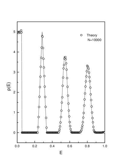
FIG. 1.: Distribution of states $p(E)$ for $k=4$ and $\epsilon=0.05$: theoretical (solid) and simulation (circles) with $N=10^{4}$ sites.

The branching ratio $\sigma$ is calculated as follows. All the sites that can be activated are in the $k$-th bump. When they are hit, sites with $E>1-\alpha$ activates deterministically. In terms of the re-scaled variable $z_{k}=E-(k-1)\alpha$, this condition refers to sites with $z_{k}>\delta\equiv 1-k\alpha$. They contribute to the branching ratio with the quantity $\sigma^{\prime}$,

$$\sigma^{\prime}\equiv k\int_{1-\alpha}^{1}p(E)dE=\int_{\delta}^{\delta+\alpha}p(z)\>dz\>,$$ (24)

where $z\equiv z_{k}$.

Sites with $z<\delta-\epsilon$ cannot be activated and does not contribute to $\sigma$. Sites with $\delta-\epsilon<z<\delta$ can be activated if they receive a quantity $\alpha+\eta$ with $\eta>\delta-z$. This occurs with probability $P(\eta>\delta-z)=1-(\delta-z)/\epsilon$. Then, these sites contribute to the branching ratio with the quantity

$$\sigma^{\prime\prime}\equiv\int_{\delta-\epsilon}^{\delta}p(z)\left(1-\frac{\delta-z}{\epsilon}\right)dz\>.$$ (25)

The total branching ratio is then

$$\sigma = \sigma^{\prime}+\sigma^{\prime\prime}=1-\int_{0}^{\delta-\epsilon}p(z)\>dz$$ (26)

$$- \frac{\delta}{\epsilon}\int_{\delta-\epsilon}^{\delta}p(z)\>dz+\frac{1}{\epsilon}\int_{\delta-\epsilon}^{\delta}z\>p(z)\>dz\>,$$ (27)

where it was used the fact that $\int_{0}^{\delta+\alpha}p(z)dz=1$. Since $p(z)$ has a simple piece-wise polynomial form (see Eq. (15)) the calculation of $\langle s\rangle$ is straightforward and the result is presented in Fig. 2 along with simulation results for the $k=4$ case with $\epsilon=0.05$.

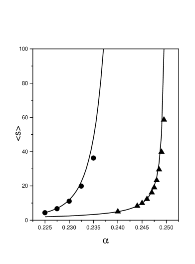
FIG. 2.: Mean avalanche size $\langle s\rangle$ as a function of parameter $\alpha$. Theoretical (solid) and simulations with $N=10^{4}$ sites for noisy EFF model (circles) with $\epsilon=0.05$ and noiseless EFF model (triangles) with $\epsilon=0.2$. These $\epsilon$ values are chosen such that the last interval ($I_{4}$) has the same length in both models.

For $\delta<\epsilon$, that is, $\alpha_{c}-\alpha<\epsilon/k$, the form assumed by $\sigma$ is particularly simple, since $p(z)=C\epsilon^{-k}z^{k-1}$ in that interval ($C$ is a numerical constant). Then,

$$\sigma = 1-\frac{C}{\epsilon^{k+1}}\int_{0}^{\delta}z^{k-1}(\delta-z)dz\>$$ (28)

$$= 1-\frac{C}{k(k+1)}\left(\frac{\delta}{\epsilon}\right)^{k+1}\>.$$ (29)

Since $\delta\equiv 1-k\alpha=k(\alpha_{c}-\alpha)$, this means that $\langle s\rangle$ diverges as $(\alpha_{c}-\alpha)^{-k-1}$, see Eq. (10). For example, for $k=4$ and $\epsilon=0.05$, $\langle s\rangle=120$ already for $\alpha=0.2375$. Curiously, this behavior is similar to the $(\alpha_{c}-\alpha)^{-k}$ divergence found in the standard random neighbor FF model [3].

E The ‘noiseless’ EFF model

It is instructive to compare this behavior with that of a simpler FF model where the firing rule is the same, $E_{i}^{*}(t+1)=\eta\in[0,\epsilon]$ but the neighbor update rule is noiseless, $E_{rn}(t+1)=E_{rn}(t)+\alpha$. Then, $p(E)$ assumes the form of $k$ rectangular bumps with $p(z_{n})=\epsilon^{-1}\Theta(z_{n})\Theta(\epsilon-z_{n})$. In this case, here called ‘noiseless’ EFF model, the branching ratio is $\sigma=0$ for $\delta>\epsilon$ and $\sigma=1-\delta/\epsilon$ for $0<\delta<\epsilon$. In contrast with the previous model, large avalanches only occur when $\alpha$ is very close to $\alpha_{c}$ (see Fig. 2).

III Comparison with the random-neighbor Bak-Sneppen model

The Bak-Sneppen model [7] consists of $N$ sites carrying real variables $x$ (fitness) that follow an extremal dynamics with the rules:

$$x_{i}^{*}\equiv\mbox{min}\{x_{j}\}\>,$$ (30)

$$x_{i}^{*}(t+1)=\eta\>,$$ (31)

$$x_{rn}(t+1)=\eta\>,$$ (32)

where $\eta$ is an uniformly random variable in the interval $[0,1]$. To facilitate the comparison with the extremal FF model, one makes a change of variables to $E=1-x$, the BS neighbor update rule may be written as $E_{rn}=\eta\in[0,A]$ (the Bak-Sneppen choice is $A=1$). Thus, the parameter $A$ is related to the effective coupling strength between neighbors.

In the $N\rightarrow\infty$ limit, its stationary distribution of states is $p(E)=\frac{k}{(k-1)A}\Theta(\frac{(k-1)A}{k}-x)$. Note that, here, $k$ is not the number of neighbors $q$ but the number of tentative branches $k=1+q$ since, in the BS model, the firing site is also a tentative branch which may contribute to $\sigma$. Thus, the random neighbor BS model presents, in the stationary state, a natural threshold at

$$\lambda_{c}=(k-1)A/k\>.$$ (33)

All firing (‘mutating’) sites have $E$ above $\lambda_{c}$, so Bak-Sneppen argued that it is natural to choice $\lambda_{c}$ as the threshold that defines avalanches. With this choice, the distribution $p(s)$ is a power law.

Like the Bak-Sneppen model, a ‘natural’ threshold $\lambda_{c}(\alpha)$ also appears in the extremal FF system. Suppose that the initial condition $p(E,t=0)$ is uniform in the interval $[0,1]$. Then, define the ‘gap’ at time $t$ as the minimal extremal site chosen up to $t$. During the transient, the gap evolves toward the value

$$\lambda_{c}(\alpha)=(k-1)\alpha+k\epsilon\>.$$ (34)

Now, if we define an avalanche as the return time between two crosses of $\lambda_{c}$ by the time series of extremal values, like is done by Bak and Sneppen, then the system will stay always critical since $\lambda_{c}$ is a function of $\alpha$ and all is the same when $\alpha$ is changed. Indeed, any choice for $\lambda$ in the interval $[\lambda_{c}(\alpha),E_{c}(\alpha)=k\alpha]$ makes the $\lambda$-avalanches critical.

Thus, the Bak-Sneppen choice for the threshold $\lambda$ as the point where $p(E)$ drops, although natural, is indeed a fine tuning operation! It corresponds, in the extremal FF model, to choose the proper $\lambda_{c}(\alpha)$ (or, alternatively, $E_{c}(\alpha)=k\alpha$) for defining avalanches. Then, in the EFF model, instead of fixing $E_{th}=1$ and fine tuning the coupling parameter to $\alpha_{c}(E_{th})=1/k$, the parameter $\alpha$ could be fixed and the threshold could be fine tuned to $E_{c}(\alpha)$ (or $\lambda_{c}(\alpha)$). The fine tuning is incorporated (hidden?) in the definition of avalanches!

Now, for comparing between the coupling strength in the FF model (in the limit $\epsilon\rightarrow 0$) and the BS model, calculate the average new value assumed by a neighbor,

$$\mbox{BS: }\langle E(t+1)\rangle = A/2\>,$$ (35)

$$\mbox{FF: }\langle E(t+1)\rangle = \langle E\rangle+\alpha=k\alpha/2\>,$$ (36)

since $\langle E\rangle=(k-1)\alpha/2$ for the FF model. Thus, to see the strong analogy between the extremal FF and the BS models, it is natural to write $A=k\alpha$ (remember, $A$ is an arbitrary parameter which controls the effective coupling between sites in the BS model). Then, Eq. (33) is $\lambda_{c}=(k-1)\alpha$ which has the same form of Eq. (34) (with $\epsilon\rightarrow 0$). This means that there is a well defined dependence of $\lambda_{c}$ on the parameter $\alpha$ which controls the coupling between sites: the definition of $\lambda_{c}$, although natural, is not robust to changes in the coupling strength. The issue here is not robustness but automatic fine tuning of the threshold $\lambda_{c}$ (see bellow).

IV On SOC definitions

The idea of self-organized criticality present in the literature embodies two distinct properties. The term self-organized refers to the fact that there exist a parameter ($\sigma(t)$), which controls the avalanche behavior, whose value is not fixed a priori like, for example, in standard percolation, but evolves during a transient phase toward an stationary value $\sigma(\infty)$. Indeed, this time dependence should be written as $\sigma(p(E,t))$, that is, $\sigma$ is a functional of the time varying distribution of states $p(E,t)$ and $\sigma(\infty)\equiv\sigma(p(E,\infty))$.

The evolution of $p(E,t)$ toward the non-equilibrium steady-state $p(E,\infty)$ is akin to the transient relaxation in equilibrium systems: any initial condition leads to the same stationary state, thus, the same value for $\sigma(\infty)$. However, this robustness to initial conditions and perturbations (‘dynamical stability’) should not be mistaken as parameter robustness (‘structural stability’). Then, a second and distinct characteristic recurrently claimed for SOC systems is structurally stable criticality [1] [5]: there exists a finite parameter range where, after the transient, the system is critical (that is, $\sigma(\infty)=\sigma_{c}$). For this situation, no fine tuning is needed to find a system with critical behavior, only some gross tuning. This kind of structurally stable criticality will be called type-I SOC.

Now, it seems that all the SOC models in the literature, at least in the random-neighbor versions or other analytically tractable situations, are not robust to changes in the coupling strength between sites. For example, it is well known that the sand pile model is not critical if there exists a non vanishing probability of a grain to evaporate during an avalanche. This probability plays a similar role of the quantity $1-k\alpha$ in the present model.

Structurally stable criticality is depicted in Fig. 3(a). In this case, by changing the coupling parameter $\alpha$, there is a finite range where $\sigma$ assumes the critical value $\sigma_{c}=1$. Standard criticality, then, may be viewed as the fine tuning dependence of $\sigma$ on $\alpha$ represented in Fig. 3(c). However, a third possibility is a strong nonlinear dependence of $\sigma(\alpha)$ (Fig 3(b)) like the observed in the noisy extremal FF model and in the standard random neighbor FF and OFC models studied in [3]. The system is almost critical in a large parameter region: this will be called generic quasi-criticality. In standard critical phenomena parlance, the system has a very large ‘critical region’. The importance of this characterization is that various systems examined in the SOC literature, previously beheld as having true generic criticality, are now being recognized as having only generic quasi-criticality in the sense defined above.

A candidate for type-I SOC is the two-dimensional OFC model [9, 10]. Of course, models defined in lattices are hard to analyze. It is not clear if the other factors present in that models (spatial structure, large probability of re-visitation of sites during an avalanche, boundary conditions etc.) create a truly generic critical state for a finite interval in the coupling parameter ($\alpha$) space or only a generic quasi-critical behavior. It seems reasonable to ask, however, why these arbitrary factors should conspire to give exactly a critical state $\sigma(\infty)=1$ instead of only amplifying the tendency toward large avalanches already present in the random-neighbor version. If the latter view is correct, then a conjecture can be made that a necessary condition for lattice models (like 2D OFC) to present an apparent generic SOC behavior is that the corresponding random-neighbor version presents strong quasi-criticality behavior.

It also has been argued that, by analogy with the extremal FF model, the Bak-Sneppen model should not be viewed as having structural stability. The choice of the threshold $\lambda_{c}$ for defining avalanches, although natural, is similar to the fine dependence $\lambda_{c}(\alpha)$ or $E_{c}(\alpha)$ in the present model. Ironically, the random-neighbor BS model is even not ‘self-organized’ in the sense defined here: with $\lambda=\lambda_{c}$ fixed, the branching ratio is always $\sigma=1$ and does not evolve during the transient phase. In contrast with the EFF model, the probability of a neighbor site to fire does not depend on its previous state, so that there is no coupling between $\sigma$ and $P(E,t)$.

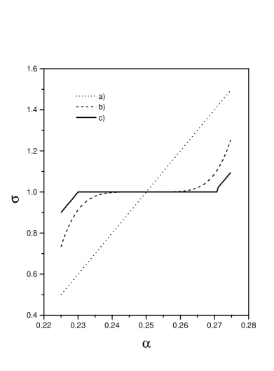
FIG. 3.: a) Structurally stable criticality: the value of parameter $\sigma$ is critical on a finite range of the system parameter $\alpha$. b) Generic quasi-criticality (noisy EFF model): the dependence of $\sigma(\alpha)$ is non-linear near $\sigma_{c}$. c) Standard criticality (noiseless EFF model): the system parameter $\alpha$ must be fine tuned for obtaining $\sigma\approx\sigma_{c}$.

Although type-I SOC (or SSC, structurally stable criticality) seems to be hard to find, another possibility consists in systems where the coupling strength $\alpha$ is not a fixed parameter but turns out a slow dynamical variable. That is, although criticality requires a fine tuning of $\alpha$, this is done automatically by some self-tuning mechanism. This will be called type-II SOC or STC (self-tuned criticality). For example, suppose that the coupling $\alpha_{ij}$ evolves as

$$\alpha_{ij}(t+1)=(1+\Omega_{1})\alpha_{ij}(t)-\Omega_{2}\Delta_{i}(t)\>,$$ (37)

with $\Omega_{1}<\Omega_{2}$, both small quantities, and $\Delta_{i}(t)=1$ if site $j$ has fired at time $t$ and $\Delta_{i}(t)=0$ otherwise. Thus, a supercritical state will present a lot of big avalanches which shall decrease the average coupling toward the subcritical regime. On the other hand, if the system is subcritical, the average $\langle\alpha_{ij}\rangle$ grows. This dynamics for the couplings has a stationary state $P(\alpha)$ that seems to produce a robust critical state [11]. Note that the coupling dynamics is local (depends only on site $i$) and does not require a fine tuning in the parameters $\Omega_{1}$ and $\Omega_{2}$.

The motivation for this dynamics may be (in the context of neural networks) an activity dependent depression in synaptic efficacy due to synaptic fatigue. In slip-stick context, this dynamics may correspond to some plastic change in the coupling mechanism between sites (for example, rupture and recover of contacts between neighbors). Systems with type-II SOC, however, have not yet been fully explored in the literature (see [11]).

V Conclusions

A class of extremal slip-stick models has been introduced. The FF model has been studied in the $N\rightarrow\infty$ limit; the model presents a clear mechanism for producing a strong divergence on the average size of avalanches like that found in another more complicated models [2, 3]. As possible extensions, one could examine finite dimensional versions of these extremal models and the use of other update rules (say, OFC rules). Preliminary results shows synchronization phenomena for the 1D case [11].

From a practical viewpoint, that is, for explaining generic scale invariance in Nature, structurally stable criticality or generic quasi-criticality are almost identical (up to a cutoff size always present in natural systems). It is, however, of interest to determine what are the basic ingredients for producing generic quasi-criticality in the models examined in the SOC literature. The simple mechanism devised in this work suggests that, if true robust criticality (type-I SOC) is not easy to be achieved, generic quasi-criticality certainly is. Perhaps, true type-I SOC do not exist, only generic quasi-criticality and, perhaps, type-II (self-tuned) criticality.

Aknowledgments: The author thanks C. P. C. Prado and S. R. A. Salinas for useful suggestions, N. Dhar for illuminating discussions about the SOC concept, J. F. Fontanari and R. Vicente for commenting the manuscript and FAPESP for financial support.

REFERENCES

- [1] P. Bak, How Nature Works (Copernicus, New York, 1996).
- [2] M-L. Chabanol and V. Hakin, Phys. Rev. E 56 R2343 (1997).
- [3] H-M. Bröker and P. Grassberger, Phys. Rev. E 56 3944 (1997).
- [4] S. Lise and H. J. Jensen, Phys. Rev. Lett. 76 2326 (1996).
- [5] G. Grinstein, in Scale Invariance, Interfaces and Criticality, Vol. 344 of NATO Advanced Study Institute, Series B: Physics, edited by A. McKane et. al (Plenum Press, New York, 1995).
- [6] H. Feder and J. Feder, Phys. Rev. Lett. 66, 2669 (1991).
- [7] P. Bak and K. Sneppen, Phys. Rev. Lett. 71 4083 (1993).
- [8] H. Flyvbjerg, K. Sneppen and P. Bak, Phys. Rev. Lett. 71 4087 (1993).
- [9] Z. Olami, H. J. F. Feder and K. Christensen, Phys. Rev. Lett. 68 1244 (1992).
- [10] P. Grassberger, Phys. Rev. E 49 2436 (1994).
- [11] O. Kinouchi, in preparation.