Numerical treatment of the hyperboloidal initial value problem for the vacuum Einstein equations
II. The evolution equations

Abstract

This is the second in a series of articles on the numerical solution of Friedrich’s conformal field equations for Einstein’s theory of gravity. We will discuss in this paper the numerical methods used to solve the system of evolution equations obtained from the conformal field equations. In particular we discuss in detail the choice of gauge source functions and the treatment of the boundaries. Of particular importance is the process of “radiation extraction” which can be performed in a straightforward way in the present formalism.

1 Introduction

In article [1] we have presented the conformal field equations explicitly in a form suitable for solving them numerically. In a brief summary, we have derived the conformal field equations in the space spinor formalism which is well suited to perform the $3+1$ split because the evolution equations come out in a symmetric hyperbolic form (under appropriate assumptions on the free gauge source functions) almost automatically. We have also discussed in [1] the further assumption of a hypersurface orthogonal symmetry which has been made to simplify the implementation. Fixed points of a continuous symmetry usually lead to coordinate singularities which have to be treated specially in any finite difference method. Therefore, we followed a suggestion of B. G. Schmidt [2] to require that there be no fixed points which has the unphysical consequence that the global topology of space-time is $T^{2}\times\mathbf{R}^{2}$. However, since the emphasis of this project lies in studying the effectiveness of radiation extraction from the numerically generated space-times and since these are local methods this is not a serious disadvantage.

In section 2 we first present the numerical method, a Lax-Wendroff method in two dimensions and the procedure for choosing the time-step dynamically in order to enforce the CFL condition for stability of the algorithm. In section 3 we show how the boundary can be treated. This is an essential part of any numerical scheme because if the boundary conditions are non-physical one has to live with the fact that the numerical solution probably differs quite significantly in the domain of influence of the boundary from what one expects it to be there. In the present approach this problem can be avoided because the boundary is entirely outside the physical space-time. From the causal properties of the evolution equations it is at least plausible that null infinity $\mathcal{J}$ which is a characteristic surface for the differential equations also numerically acts as a barrier for perturbations generated in the unphysical space-time.

The section 4 is devoted to a discussion of the various gauge source functions. This is an important subject also in the conventional treatments of the Einstein equations because it is not clear what the implications are if one chooses e.g. the lapse function and the shift vector in that way and not in another. The existence of $\mathcal{J}$ imposes some questions concerning the resolution of features inside the physical space-time during the course of the computation. But these questions can be solved completely satisfactorily by making use of a certain choice of shift vector which is forced by the structure of conformal field equations.

Finally, in section 5 we discuss the procedure of “radiation extraction”. By this term we mean the determination of certain asymptotic quantities which in a well defined sense characterise the gravitational radiation generated inside the physical space-time and escaping out to infinity. Here, this is a well defined procedure which involves finding the zero-set of the conformal factor, the interpolation of the field variables and a frame transformation to a well defined frame which is adapted to the geometry of $\mathcal{J}$. Another issue discussed in this section is the determination of the Bondi mass. Here, due to the different global topology, the situation is different from the physical one in that one cannot find a Bondi four-momentum but only a Bondi scalar.

We tested the code by using exact solutions to first provide initial data for all the variables and then to compare the computed variables with the analytic ones. We also computed the radiative quantities from the exact solutions for comparison with the numerically determined ones to check the radiation extraction method.

As in [1] we use the conventions of [3] throughout.

2 The numerical evolution scheme

The evolution part of the conformal field equations presented in [1, section LABEL:sec:eqns] with the symmetry reduction described in [1, section LABEL:sec:symm] are to be solved numerically. To this end we set up a two-dimensional grid with coordinates $u,v$. It is assumed that the fields are periodic in $u$ with period 2 so that we need to impose periodic boundary conditions at the surfaces $u=\pm 1$. The coordinate $v$ takes values in the interval $\left[-v_{0},v_{0}\right]$. The question of boundary conditions at the surfaces $v=\pm v_{0}$ is rather delicate from the numerical point of view and will be discussed in detail in section 3.

Having set up the grid we need to obtain solutions of the constraint equations in order to initialise the fields. This should be done by solving the constraint equations numerically given the appropriate free data and boundary data. However, since we are here concerned mainly with the evolution algorithm we will simply take these initial values from appropriately adapted exact solutions which have recently been pointed out by Schmidt [2]. In particular, we take the rescaled A3 solution and one other solution from this class (see appendix A) in various gauges as our test case.

As our numerical method for solving the evolution equations we choose finite difference schemes which are second order accurate in both time and space. In particular, we use the leapfrog and the Lax-Wendroff schemes both extended in a straightforward manner to two space dimensions. Of course, various other methods could have been employed. It soon becomes apparent that the leapfrog method is not a viable choice in our case. Since the conformal field equations form a quasi-linear symmetric hyperbolic system it follows that the characteristics which determine the evolution of the fields depend on the solution itself. Or, to put it differently, the wave parts of the fields propagate along the light cone which is determined by the metric which, in turn, is evolved by the field equations. Since the methods we employ are explicit we need to make sure that they remain stable by controlling the size of the time step $\Delta t$ during the evolution. However, changing the time step dynamically cannot be done with the leapfrog method without loosing the second order accuracy in time. Hence, we will focus here exclusively on the Lax-Wendroff method.

The equations in the general form given in [1, section LABEL:sec:eqns] are manipulated using the NPspinor package [4] of Maple, extended to include the space spinor formalism. The equations are expanded into components using the decomposition into irreducibles for each spinor field. We should point out that the equations when written in components turn into, in general, complex equations for complex variables. Due to the reality properties of the spinor fields these equations come either in complex conjugate pairs or as real equations. This fact reduces the number and the complexity of the equations. The symmetry conditions given in [1, section LABEL:sec:symm] are used to simplify them. Maple is also used to test the equations thus obtained quite extensively in various ways:

• They are checked against hand calculations in simple enough cases.

• Inserting exact solutions into the equations should result in identities. These solutions are obtained also with the help of Maple using different routines by conformally transforming simple vacuum solutions of Einstein’s equations with arbitrary conformal factors.

• The most important test, however, is the fact that the evolution equations have to propagate the constraints. This property was verified for the full expanded evolution equations and constraints using Maple.

The two-dimensional Lax-Wendroff scheme is a straightforward generalisation of the one dimensional case. For a quasi-linear equation of the form

$$f_{t}=A(t,u,v,f)f_{u}+B(t,u,v,f)f_{v}+E(t,u,v,f)$$ (2.1)

it can be characterised as follows. Define the following operators acting on a grid function $f_{i,j}$

$$\mu_{1}[f]_{i,j} =\frac{1}{2}\left(f_{i-\frac{1}{2},j}+f_{i+\frac{1}{2},j}\right), \mu_{2}[f]_{i,j} =\frac{1}{2}\left(f_{i,j-\frac{1}{2}}+f_{i,j+\frac{1}{2}}\right),$$ (2.2)

$$D_{1}[f]_{i,j} =\left(f_{i+\frac{1}{2},j}-f_{i-\frac{1}{2},j}\right), D_{2}[f]_{i,j} =\left(f_{i,j+\frac{1}{2}}-f_{i,j-\frac{1}{2}}\right).$$ (2.3)

Then the 2D-Lax-Wendroff scheme consists of the four steps

$$\bar{f}^{n}_{i+\frac{1}{2},j+\frac{1}{2}} \leftarrow\frac{1}{2}\mu_{1}\left[\mu_{2}\left[f^{n}\right]\right]_{i+\frac{1}{2},j+\frac{1}{2}},$$

$$f^{n+\frac{1}{2}}_{i+\frac{1}{2},j+\frac{1}{2}} \leftarrow\bar{f}^{n}_{i+\frac{1}{2},j+\frac{1}{2}}+\frac{1}{2}C_{u}A^{n}_{i+\frac{1}{2},j+\frac{1}{2}}\mu_{2}\left[D_{1}\left[f^{n}\right]\right]_{i+\frac{1}{2},j+\frac{1}{2}}$$

$$+\frac{1}{2}C_{v}B^{n}_{i+\frac{1}{2},j+\frac{1}{2}}\mu_{1}\left[D_{2}\left[f^{n}\right]\right]_{i+\frac{1}{2},j+\frac{1}{2}}+\frac{1}{2}\Delta t\,E^{n}_{i+\frac{1}{2},j+\frac{1}{2}},$$

$$\bar{f}^{n+\frac{1}{2}}_{i,j} \leftarrow\frac{1}{2}\mu_{1}\left[\mu_{2}\left[f^{n+\frac{1}{2}}\right]\right]_{i,j},$$

$$f^{n+1}_{i,j} \leftarrow f^{n}_{i,j}+C_{u}A^{n+\frac{1}{2}}_{i,j}\mu_{2}\left[D_{1}\left[f^{n+\frac{1}{2}}\right]\right]_{i,j}$$

$$+C_{v}B^{n+\frac{1}{2}}_{i,j}\mu_{1}\left[D_{2}\left[f^{n+\frac{1}{2}}\right]\right]_{i,j}+\Delta t\,E^{n+\frac{1}{2}}_{i,j}.$$

where $C_{u}=\frac{\Delta t}{\Delta u}$ and $C_{v}=\frac{\Delta t}{\Delta v}$ and where $A^{n}_{i+\frac{1}{2},j+\frac{1}{2}}=A(t_{n},u_{i}+\frac{1}{2}\Delta u,v_{j}+\frac{1}{2}\Delta v,\bar{f}^{n}_{i+\frac{1}{2},j+\frac{1}{2}})$ and $A^{n+\frac{1}{2}}_{i,j}=A(t_{n},u_{i},v_{j},\bar{f}^{n+\frac{1}{2}}_{i,j})$. The further generalisation of this scheme to three dimensions is straightforward. However, it becomes rather inefficient and it is here where probably operator splitting methods should be used. The complete discretisation of the equations was also carried out symbolically.

The exact solutions described in appendix A have been used to provide the initial data and (in some cases) those boundary data which can be specified freely. It is clear from the form of the metric that these solutions have two space-like Killing vectors. The Killing vector $\partial_{y}$ is taken to be the one that is factored out by the symmetry reduction (see [1, section LABEL:sec:symm]). The metric functions are independent of $x$ and $y$. If we choose $z$ and $x$ to correspond to the two remaining coordinates $v$ and $u$ respectively then the code is essentially a one-dimensional code. In order to test the two-dimensional performance of the code we therefore have to “warp” the coordinates. Thus, we put

$$x=u,\qquad z=v-\alpha(v_{0}^{2}-v^{2})\sin(\pi u).$$ (2.4)

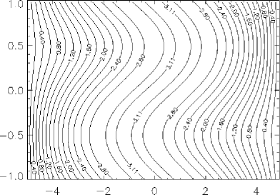
Figure 1: The orbits of the additional Killing vector $\partial_{u}$

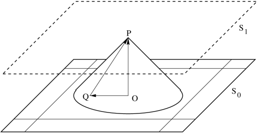
Figure 2: The local geometry for the timestep criterion

We choose $\alpha$ in such a way that this transformation is bijective in the range $u\in[-1,1],v\in[-v_{0},v_{0}]$. In this coordinate system the orbits of the second Killing vector are distorted and not aligned with the grid, see Fig. 1. All computations which are presented here have been performed with these warped coordinates. We will now describe the criterion to determine the maximal time step $\Delta t$ possible to evolve from an initial time level $\mathcal{S}_{0}$ at time $t=t_{n}$ to the next time level $\mathcal{S}_{1}$ at time $t=t_{n}+\Delta t$. This is not specific to the Lax-Wendroff method but can be used with any explicit evolution scheme. The Courant-Friedrichs-Lewy condition [5] can be phrased as stating that “the numerical domain of dependence should enclose the analytical domain of dependence”. Now consider a point $P$ in the future time level (cf. fig. 2). Its numerical domain of dependence consists of the points at time $t_{n}$ which are used to compute the field values at $P$. They lie within a rectangular area $\mathcal{R}$ bounded by coordinate lines $u=u_{\pm}$ and $v=v_{\pm}$. The analytic domain of dependence is given by the intersection of the backward light cone of $P$ with the time slice $\mathcal{S}_{0}$. The maximal allowed time-step $\Delta t$ is therefore at most so big that the light cone just touches the boundary of $\mathcal{R}$. To obtain a formula for the maximal $\Delta t$ we analyse this situation to first order or, what is the same thing, in Minkowski space. Then the time levels are planes and the light cone is a true cone, the null cone of the point $P$. Let $O$ be the point in $\mathcal{S}_{0}$ which is “straight below” $P$ in the sense that $\overrightarrow{OP}$ is a multiple of the normal vector $t^{a}$ of $\mathcal{S}_{0}$. We take $O$ as the origin. Let $Q$ be the point in $\mathcal{S}_{0}$ with the same spatial coordinates as $P$ so that $\overrightarrow{QP}=\Delta t\partial_{t}$. The equation for the plane $\mathcal{S}_{1}$ is given by $\langle dt,x\rangle=\langle dt,\overrightarrow{QP}\rangle=\Delta t$ so that $\overrightarrow{OP}^{a}=Nt^{a}\Delta t$. Then $\overrightarrow{OQ}$ is proportional to the shift vector $\overrightarrow{OQ}=-N\Delta tT^{i}\partial_{i}$. The equation for the null cone of $P$ is

$$g_{ab}\left(x^{a}-\overrightarrow{OP}^{a}\right)\left(x^{b}-\overrightarrow{OP}^{b}\right)=0$$ (2.5)

and its intersection $E$ with $\mathcal{S}_{0}$ is given by all points $x^{a}$ which obey the equations

$$t_{a}x^{a}=0,\qquad x^{a}x_{a}=2N^{2}\Delta t^{2}=0.$$ (2.6)

Now we take any plane $H$ orthogonal to $\mathcal{S}_{0}$, whose equation is $\omega_{a}x^{a}=s$ for some $\omega$ with $\omega_{a}t^{a}=0$ and arbitrary $s$. Suppose that $H$ touches $E$ in a point $X$. Then, at $X$ the following equations hold:

$$x^{a}=\overrightarrow{OX}^{a},\quad x^{a}x_{a}=-2N^{2}\Delta t^{2},\quad\omega_{a}x^{a}=s,\quad x_{a}=\alpha\omega_{a}.$$ (2.7)

The last equation expresses the fact that the tangent plane at $X$ to $E$ in $\mathcal{S}_{0}$ is parallel to the intersection of $H$ with $\mathcal{S}_{0}$. From these equations, one can easily derive the relations

$$2N^{2}\Delta t^{2}\omega_{a}\omega^{a}=-s^{2},$$ (2.8)

$$x^{a}=-\frac{2}{s}N^{2}\Delta t^{2}\omega^{a}.$$ (2.9)

We are interested in coordinate planes within $\mathcal{S}_{0}$. These are obtained from $\omega=dx^{i}-NT^{i}dt$. In particular, we consider coordinate planes which are a distance $\pm\Delta x^{i}$ from the point $Q$. These satisfy the equation $\omega_{a}x^{a}=-NT^{i}\Delta t\pm\Delta x^{i}$. Inserting this value for $s$ in the equations above we obtain the equation

$$\left(T^{i}\pm\sqrt{-2\omega_{a}\omega^{a}}\right)N\Delta t=\pm\Delta x^{i},$$ (2.10)

which holds whenever the past light cone of $P$ touches a coordinate plane which is $\pm\Delta x^{i}$ from the point $Q$. Thus, according to our criterion, a valid time-step $\Delta t$ should satisfy

$$\Delta t\leq\mathrm{min}\frac{\Delta x^{i}}{N|T^{i}\pm\sqrt{-2\omega_{a}\omega^{a}}|},$$ (2.11)

where the minimum is taken over all points in $\mathcal{S}_{0}$. There are some points to be mentioned:

• In our present case the square root is simply $\sqrt{-2\omega_{a}\omega^{a}}=2\sqrt{C_{AB}^{i}C^{ABi}}$, so that determining the maximal time-step is rather simple. It involves going through the grid and finding the maximum of some algebraic function of the fields (no inversion of the spatial metric).

• We find that the criterion is at least necessary for stability, i.e., if we do not enforce the time-step to be at most the above value then the scheme becomes unstable. So far it has also been sufficient for stability.

• This criterion might be conservative. In fact, one could imagine that one should be able to increase the time step until the first of the adjacent grid points comes to lie on the null cone, the others still being not inside. We have not investigated this further.

• This is a first order criterion and it might be too crude for the Lax-Wendroff method. One could think of enforcing this condition at each half step. Again this has not been investigated.

A complete time step is performed by going through the following steps given the solution at the time level $t_{n}$

• Find the maximal possible time step $\Delta t$ by inspection of the current time level.

• Set the gauge functions, also possibly according to the properties of the solution at the current time level.

• Update the solution at the interior points using the gauge functions and the time-step by performing the above four steps for each function. After the first half step specify the gauge source functions again.

• Update the solution at the boundary points.

3 Boundary treatment

Analytically, the hyperboloidal initial value problem does not need any boundary conditions. The initial data are given on a three dimensional manifold $\mathcal{S}$ with boundary $\partial\mathcal{S}$ on which the conformal factor $\Omega$ is supposed to vanish. Then a solution exists on the four dimensional manifold $M=\mathcal{S}\times\left[0,\tau\right]$ for some $\tau>0$ which is such that the boundary $\partial M=\partial\mathcal{S}\times\left[0,\tau\right]$ is a null hypersurface and hence characteristic. That means that even if one would extend the initial data across the boundary $\Omega=0$ in some way this extension could not influence the interior, i.e., the physical space-time depends only on the data given inside the boundary.

The situation is different in the numerical case. The characteristic speeds are different for different modes which are propagated by the numerical scheme. In particular, non-physical modes tend to propagate at speeds much higher than physical propagation speeds and thus contaminate the solution all over the entire computational domain. A notorious place where non-physical modes are generated is at the boundaries of the domain. Due to the lack of enough grid points there, in general, the numerical evolution scheme has to be changed. It is absolutely vital to impose boundary conditions so that the non-physical modes are kept small. The GKS theory [6, 7] which has been developed for analysing such situations is inherently difficult to apply. A different (equivalent) formulation based on the notion of group velocity for finite difference schemes has been given by Trefethen [8]. It has been found that certain intuitive numerical boundary conditions do not perform as expected. Conditions which work for one numerical scheme do not necessarily work for others. For linear equations in one space dimension the mathematical analysis can completely be carried through. It turns out that the essential criterion is a non-degeneracy condition for a linear system of equations obtained from the combination of the evolution scheme and the boundary condition. This system is required to have no solutions in order to exclude the parasitic modes. Although Trefethen’s method is very physical and intuitive it does not provide enough information in the case of higher dimensional and/or non-linear equations. It does, however, give valuable hints as to which conditions might have a chance to be useful in those more general situations treated with the Lax-Wendroff scheme.

The situation is somewhat ironic in the present case. One is not at all interested in what happens at the boundary because this is (usually) outside the physical space-time. However, it is the boundary which needs the most careful treatment. One would wish to find gauge conditions which make the non-physical portion of the computational domain small, ideally putting the boundary at $\Omega=0$. We will examine the feasibility of this idea later on.

In another aspect, the present situation is also quite disadvantageous. Usually, it is of great importance that the analytical problem has a well posed initial-boundary value problem. The rigorous analysis provides the information about which data can be specified freely at the boundary and which data is determined from information propagating towards the boundary from the inside. Knowledge of this kind is necessary in order not to over-specify the solution at the boundary, because this would inevitably lead to instabilities (except for extremely simple cases). In our case, it is not known at present whether the system admits a well posed initial-boundary value problem (see, however [9]). To overcome this lack of information we analyse the system to first order at the boundary in the following sense.

The boundary $\mathcal{B}$ is a time-like three-dimensional hypersurface in the space-time. Let $n_{a}$ be the space-like conormal of $\mathcal{B}$. A system of partial differential equations which has the form

$$\partial_{t}u_{\alpha}+A^{i}_{\alpha\beta}\partial_{i}u^{\beta}=b_{\alpha}$$ (3.1)

can be rewritten in the form

$$\partial_{t}u_{\alpha}+C_{\alpha\beta}\mathcal{D}u^{\beta}+B^{A}_{\alpha\beta}\partial_{A}u^{\beta}=b_{\alpha},$$ (3.2)

where $\mathcal{D}$ is the derivative along any vector field $u^{a}$ which satisfies $n_{a}u^{a}=1$ on $\mathcal{B}$ (usually taken to be the normal vector field extended off $\mathcal{B}$ in an arbitrary way) and where the $\partial_{A}$ are derivatives intrinsic to $\mathcal{B}$ at points of $\mathcal{B}$. On the boundary the matrix $C_{\alpha\beta}$ regulates to first order the propagation of the fields across the boundary. By analysing its structure one can gain valuable insights into the behaviour of the solution on $\mathcal{B}$. In particular, finding the eigenvalues and eigenvectors of $C_{\alpha\beta}$ (which in our case is hermitian) enables us to select combinations of the fields which (to first order) propagate purely inward or purely outward or which stay on the boundary. These have to be treated differently. While the ingoing pieces can be prescribed freely, the outgoing ones have to be obtained from the interior. This is done here by extrapolation. That this might be possible is indicated be the Trefethen analysis which shows that extrapolation remains stable when used in conjunction with the one-dimensional Lax-Wendroff method. We want to mention that this analysis applies not only at the boundary but also at the interfaces between grid cells. This is important for possible future application of high resolution methods which require the solution of Riemann problems at each grid cell, see e.g., [10].

To be somewhat more precise we need to analyse the three subsystems of the full system which do not consist entirely of advection equations along the $\partial_{t}$ vector. These are the systems for the variables $\left(K_{ABCD},K_{AB},K\right)$, the variables $\left(\phi_{ABCD},\phi_{AB},\phi\right)$ and for the Weyl curvature $\left(E_{ABCD},B_{ABCD}\right)$, respectively. Note, that this analysis is valid in the three-dimensional case. Only in the code we have specialized this to the two-dimensional case. Let us describe the procedure for the $\phi$-system.

First, we note that $n_{a}=n_{AB}$ can be viewed as a complex metric on spin space which reduces the structure group from $SL(2,\mathbf{C})$ down to $U(1)$. Thus, it is possible to decompose any symmetric spinors $\Phi_{AB}$, $\Phi_{ABCD}$ into irreducible pieces with respect to the smaller structure group:

$$\Phi_{AB} =\Phi_{AB}^{(0)}-\frac{1}{2n^{2}}n_{AB}\Phi^{(1)},$$ (3.3)

$$\Phi_{ABCD} =\Phi_{ABCD}^{(0)}-\frac{1}{n^{2}}n_{(AB}\Phi_{CD)}^{(1)}+\frac{3}{8n^{4}}n_{(AB}n_{CD)}\Phi^{(2)},$$ (3.4)

where $n_{AB}n^{AB}=-2n^{2}$ and

$$\Phi^{(1)} =\Phi_{AB}n^{AB},$$ (3.5)

$$\Phi^{(2)} =\Phi_{ABCD}n^{AB}n^{CD},$$ (3.6)

$$\Phi^{(1)}_{AB} =\Phi_{ABCD}n^{CD}+\frac{1}{2n^{2}}n_{CD}\Phi^{(2)}.$$ (3.7)

This decomposition which is very natural algebraically corresponds geometrically to a decomposition of the fields into parts which are vertical and tangential to $\mathcal{B}$. The principal part of the $\phi$-system which does not contain tangential derivatives is

$$\partial\phi_{ABCD}-n_{(AB}\mathcal{D}\phi_{CD)},$$ (3.8)

$$\partial\phi_{AB}-\frac{2}{3}n_{AB}\mathcal{D}\phi+n^{CD}\mathcal{D}\phi_{ABCD},$$ (3.9)

$$\partial\phi+2n_{AB}\mathcal{D}\phi^{AB}.$$ (3.10)

Here we have neglected terms containing derivatives of $n_{AB}$ because those do not alter the symbol of the subsystem. Inserting the decompositions of the variables we get the following system

$$\partial\phi+2\mathcal{D}\phi^{(1)},$$ (3.11)

$$\partial\phi^{(1)}+\frac{4}{3}n^{2}\mathcal{D}\phi+\mathcal{D}\phi^{(2)},$$ (3.12)

$$\partial\phi^{(2)}+\frac{4}{3}n^{2}\mathcal{D}\phi^{(1)},$$ (3.13)

$$\partial\phi_{AB}^{(0)}+\mathcal{D}\phi_{AB}^{(1)},$$ (3.14)

$$\partial\phi_{AB}^{(1)}+n^{2}\mathcal{D}\phi_{AB}^{(0)},$$ (3.15)

$$\partial\phi_{ABCD}^{(0)}.$$ (3.16)

Obviously, this system can be decomposed into three smaller subsystems and it can be shown that the coefficient matrix of the $\mathcal{D}$ operator is hermitian with respect to a suitable inner product (it has to be because it comes from a symmetric hyperbolic system). Now it is easy to find “characteristic combinations” of the variables so that the symbol becomes diagonal, i.e., it has the form

$$\partial C+\lambda\mathcal{D}C$$ (3.17)

for each characteristic quantity. These combinations are unique only up to a scaling factor. We choose the following quantities with their respective characteristic speeds

$$C_{0} =4n^{2}\phi-6\phi^{(2)}, \lambda =0$$ (3.18)

$$C_{\pm} =4n^{2}\phi\pm 3\sqrt{4n^{2}}\phi^{(1)}+3\phi^{(2)}, \lambda =\pm\sqrt{4n^{2}}$$ (3.19)

$$C_{AB}^{\pm} =\phi_{AB}^{(1)}\pm\sqrt{n^{2}}\phi_{AB}^{(0)}, \lambda =\pm\sqrt{n^{2}}$$ (3.20)

$$C_{ABCD} =\phi_{ABCD}^{(0)}, \lambda =0.$$ (3.21)

In an analogous way we find the characteristic quantities for the $K$-system

$$C_{0} =3K^{(2)}+4n^{2}K, \lambda =0$$ (3.22)

$$C_{\pm} =6K^{(2)}\pm 3\sqrt{4n^{2}}K^{(1)}+4n^{2}K, \lambda =\pm\sqrt{4n^{2}}$$ (3.23)

$$C_{AB}^{\pm} =2K_{AB}^{(1)}\pm\sqrt{2n^{2}}K_{AB}^{(0)}, \lambda =\pm\sqrt{2n^{2}}$$ (3.24)

$$C_{ABCD} =K_{ABCD}^{(0)}, \lambda =0.$$ (3.25)

The Weyl system has a completely different structure from the previous two subsystems. Nevertheless, the analysis yields characteristic quantities written in terms of the complex Weyl spinor $\psi_{ABCD}$ and the spinor field $\varphi_{ABCD}=n_{(A}{}^{E}\psi_{BCD)E}$.

$$C_{0} =\psi^{(0)}, \lambda =0$$ (3.26)

$$C_{AB}^{\pm} =\pm\sqrt{n^{2}}\psi_{AB}^{(1)}-\varphi_{AB}^{(1)}, \lambda =\pm\sqrt{n^{2}}$$ (3.27)

$$C_{ABCD}^{\pm} =\pm\sqrt{n^{2}}\psi_{AB}^{(0)}-2\varphi_{AB}^{(0)}, \lambda =\pm\sqrt{4n^{2}}.$$ (3.28)

In our case, the boundary is given as a surface $v=\textrm{const}$ so that we can put $n_{AB}=C_{AB}^{2}$. Let us now focus on (3.17). Inserting the explicit expressions for the derivatives this is

$$\partial_{t}C+N\left(-T^{2}\partial_{v}C+\lambda\partial_{v}C\right)$$ (3.29)

Therefore, it is the sign of $\left(\lambda-T^{2}\right)$ which regulates in which direction the quantity $C$ propagates across the boundary.

To update the values at the boundary points we proceed as follows. First we determine the characteristic quantities on the boundary. This is done by looking at the sign of the corresponding eigenvalues which decides whether to simply set the value arbitrarily in case the quantity propagates inwards or else whether to find the value by extrapolation from the interior. From the characteristic quantities we obtain the field values by reversing the transformations above.

In the situations considered this procedure yields a stable algorithm. This is consistent with the Trefethen theory which shows that in the one-dimensional case extrapolation together with the Lax-Wendroff time evolution scheme remains stable. By its very nature our procedure is a first order approximation to the real situation so that we cannot expect to obtain a code which is second order accurate in the neighbourhood of the boundary. However, since the surface $\Omega=0$ is a characteristic surface we may hope, that the error does not too severely influence the physical space-time as long as the boundary of the computational domain is outside the physical space-time.

4 Gauge choices

In this section we want to present some results about the various possible gauge choices. Our emphasis will be on the temporal gauge choices. There is one class of choices for the shift vector which is natural in the present context of the conformal field equations. The gauge for the frame rotations and the third class of gauges, namely the choice of the scalar curvature $\Lambda$, is unknown territory as of yet and we put the corresponding gauge source functions equal to zero in the code. As was pointed out in I, in the case of the frame rotations this means that the frame is Fermi-Walker transported along the normal vector of the time foliation.

4.1 Choices of lapse

Let us start with the temporal gauges. Fixing the lapse function is a difficult task. This function has to be chosen in such a way that the time coordinate does not degenerate in the course of the evolution. Here is an attempt to collect some criteria which should be satisfied by the lapse:

• the lapse function should not “collapse” in the sense that it approaches zero in a finite coordinate time,

• the surfaces of constant time should remain smooth,

• the lines of constant spatial coordinates should not intersect,

• the lapse function should remain positive,

• it should not develop too steep gradients,

• depending on the problem the foliation should or should not avoid singularities.

In our treatment of the hyperboloidal initial value problem, the lapse function cannot be chosen directly. Instead it is governed by an evolution equation which contains the “harmonicity” $F=2\Box t$ as an arbitrary function of the coordinates. It is not easy to find a function $F$ which allows the lapse to satisfy some or all of the above criteria. The reason is that one has no idea what $F$ should look like in coordinates which are constructed as the code moves along. To make the lapse satisfy the criteria above one needs a certain amount of “feedback” i.e., information about the current status of the evolution seems to be unavoidable. This means, that one should specify $F$ as a function of the field variables. But since in the system also the derivatives of $F$ appear this leads to the problem that the characteristics of the system change because the symbol has been altered. We will discuss this later in this section.

The various choices for $N$ that have been considered so far are

• the “natural gauge” for the exact solutions obtained by setting $F$ equal to the expression computed from the explicit form of the metric (cf. appendix A) and variations thereof,

• the “Gauß gauge” which is the condition that $N$ should be constant throughout the timeslice,

• the harmonic gauge with $F=0$ and

• the special class of gauges for which $F$ is a function of $N$ and $K$ only, $F=f(N,K)$, which in fact includes all of the above gauges.

The popular “maximal gauge” where one requires $K=0$ probably cannot be achieved by specifying $F$.

We can judge the effects of these gauges by monitoring the function $\tau$ which satisfies the eiconal equation $\nabla_{a}\tau\nabla^{a}\tau=1$ and the condition $\tau=0$ on the initial surface. The value of this function at a point $P$ gives the distance in proper time between $P$ and the intersection point of the geodesic through $P$ tangent to the unit normal of the foliation and the initial surface. This function is evolved simultaneously with the other field variables. For the A3 solution the proper time distance from a point on the initial surface $t=t_{0}$ with $z=0$ and the singularity at $t=z=0$ is $\tau=2\sqrt{-t_{0}}$ for $t_{0}\leq 0$ and we can compare how far the evolution proceeds with the various gauge choices. In all the examples presented in this section a $100\times 100$ grid was used and the coordinate system is one discussed in section 2 with $v_{0}=5$. The initial data were taken from the exact A3 solution at an initial time $t_{0}=-5$. The boundary values were specified depending on the cases considered. When the “natural gauge” was used the ingoing boundary data were taken from the A3 solution. In all other cases these values were used initially to satisfy the corner conditions and then specified to decrease exponentially, so that after approximately 20 timesteps the ingoing values are zero.

4.1.1 $F$ as a function of the space-time coordinates

For the “natural gauge” we find that we can in principle approach the singularity arbitrarily closely by increasing the resolution appropriately. Obviously, there are hard limits imposed on the calculation by the finite precision arithmetic so that eventually the numbers will overflow.

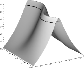
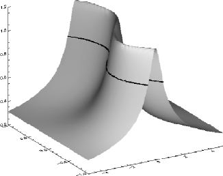
Figure 3: The proper time $\tau$ (left) and the lapse $N$ (right) in the “natural” gauge. The extremal values are $\tau_{\mbox{min}}=1.831$, $\tau_{\mbox{max}}=2.988$ and $N_{\mbox{min}}=0.315$, $N_{\mbox{max}}=1.151$. The black contours show the locations of the two $\mathcal{J}$’s.

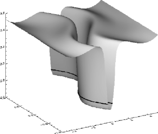
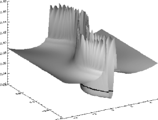
Figure 4: The proper time $\tau$ (left) and the lapse $N$ (right) in the harmonic gauge. The extremal values are $\tau_{\mbox{min}}=2.747$, $\tau_{\mbox{max}}=3.537$ and $N_{\mbox{min}}=0.03964$, $N_{\mbox{max}}=0.1624$. The zig-zag behaviour in the figure for $N$ is due to a lack of sufficient resolution for the shading process.

The difference between the natural and the harmonic gauge is shown in Fig. 3 and Fig. 4. In both figures we show the proper time $\tau$ and the lapse at a late instant of the time evolution. For the natural gauge this was dictated by the code which stopped because the time step could not be chosen without violating the CFL condition. This is due to the closeness of the singularity. The light cones are infinitely stretched along the symmetry directions as the singularity is approached. A better resolution would have extended the evolution time somewhat more but eventually the same thing would happen. In this run the coordinate time elapsed was roughly 4.405. It is clear that with this temporal gauge the singularity can be reached (at least in principle).

With harmonic gauge the code was stopped after an elapsed coordinate time 20.07. In Fig. 4 it can be seen that the evolution close to the singularity has slowed down considerably. The proper time in the center is much smaller than for regions further outside. The lapse function is very small in the center and it is decreasing. It is not known whether the evolution will reach the singularity even in principle. The decrease in the lapse could be so rapid that the integrated proper time along the central geodesic would reach a limit below the value $2\sqrt{-t_{0}}$. It is quite likely, that in this gauge the code will ultimately not be able to resolve the steep gradients which occur at late times between the interior region which cannot progress beyond the singularity and the exterior region which can.

Related to this phenomenon is the fact that the interior region shrinks. On the initial surface $\mathcal{J}$ is located at the boundary of the grid and it gradually moves inward during the evolution. Ultimately, there will be only very few grid points left in the interior region. This is a phenomenon which has nothing to do with the temporal gauge but with the choice of the shift vector. We will discuss later in this section a shift gauge which allows the freezing of $\mathcal{J}$ on the grid.

To get some feeling for the influence of $F$ on the time slicings we study the slicings obtained from substituting $p\cdot F$ for $F$ with some parameter $p$. For $p=0$ we have the harmonic gauge which avoids the singularity. For $p=1$ we have the natural gauge which allows us to reach the singularity in finite time. What happens when we increase $p$ beyond unity?

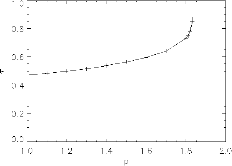
Figure 5: Proper time $\tau$ as a function of the parameter $p$

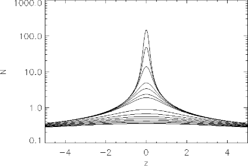
Figure 6: Profiles of the lapse N for a fixed value of the Killing coordinate $x$ and different values of $p$. Note the logarithmic scale.

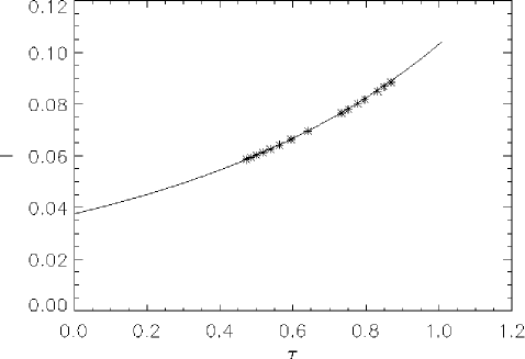
Figure 7: The curvature invariant $I$ along $z=0$ as a function of proper time. The line is the exact function, the points indicate computed values.

We evolve for a fixed coordinate time interval $t\in[-5,-4]$ with different values of $p\in\left[1.0,1.8315\right]$. We find that for $p>1.8315$ the code crashes. It is easily seen that this crash cannot be due to the curvature singularity in the A3 solution but is a coordinate singularity. In Fig. 5 we plot the proper time distance between the initial and final time slice along the central geodesic ($z=0$) versus the parameter $p$. We see that $\tau(p)$ has an infinite derivative at $p=1.8315$ with a finite value of $\tau$ far from its value $2\sqrt{5}$ at the singularity. The lapse function $N$ for different values of $p$ diverges rapidly (cp. Fig. 6). The curvature invariant $I=\Omega^{2}\left(E_{0}E_{4}+6E_{2}^{2}\right)$ which diverges at the singularity stays perfectly regular. Fig. 7 shows the exact invariant plotted against proper time along the central geodesic. The dots are the values of $I$ and $\tau$ obtained from the runs with different parameter values. We see that the behaviour of these functions is not altered by the occurrence of the coordinate singularity.

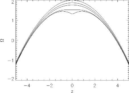
Figure 8: Profiles of the conformal factor $\Omega$ for some values of the parameter $p$

Finally, we show in Fig. 8 the profiles of the conformal factor for various values of $p$. As the parameter approaches its final value the conformal factor develops a minimum at the center. Although this behaviour seems strange at first sight it can easily be explained. The conformal factor decreases as a function of $\tau$ for fixed spatial coordinates. Due to the rapid divergence of the lapse the proper time at $z=0$ is much larger than in the regions outside. So that we see values of $\Omega$ in the center which are reduced over proportion from the values outside the center. This accounts for that central dip.

4.1.2 The Gauß gauge

The “Gauß gauge” which forces $N$ to be constant is a condition which is imposed on the lapse function directly. In principle, it is possible to express the exact solutions in Gauß coordinates by performing the coordinate transformation explicitly. Then one can compute the “harmonicity” for these coordinates and do the evolution. However, we proceed somewhat differently to impose the Gauß gauge. The lapse function satisfies the evolution equation [1, (LABEL:eq:evN)]

$$\hat{\partial}N=-N^{2}K-N^{3}F$$ (4.1)

where $\hat{\partial}=N\partial$. Now suppose that $N$ would satisfy an evolution equation

$$\hat{\partial}N=\alpha(\bar{N}-N),$$ (4.2)

where $\bar{N}$ is an arbitrary (positive) constant. This equation has the solution $N(s)=\bar{N}+N_{0}e^{-\alpha s}$, $s$ being the parameter with $\hat{\partial}s=1$. Thus, for $\alpha>0$ the lapse $N$ approaches the constant value $\bar{N}$ in the course of the evolution. We can make $N$ satisfy the above evolution equation (4.2) by choosing

$$F=\frac{\alpha(\bar{N}-N)+N^{2}K}{N^{3}}.$$ (4.3)

We find what one would expect, namely that in this gauge the timeslices develop caustics (or, what has become known as “coordinate shocks”). This makes the Gauß gauge inappropriate for long time evolutions.

4.1.3 $F$ as a function of $N$ and $K$

Let us now focus on the class of gauges defined by $F=f(N,K)$. Among this class there is a subclass for which the lapse depends only on the three-dimensional volume (-element) $V$, $N=g(V)$. For these gauges, we have with appropriate assumptions on the function $g$

$$\partial N=g^{\prime}(V)\,\partial V=-Kg^{\prime}(V)\,V=-Kg^{\prime}(g^{-1}(N))\,g^{-1}(N),$$ (4.4)

so that, in fact, $F$ is a function of $N$ and $K$ only. The natural gauge falls into this subclass with $g(x)=x^{-\frac{1}{3}}$ and, consequently, $F=-\frac{4K}{3N}$. Similarly, the harmonic gauge with $F=0$ is in this class with $g(x)\propto x$.

If we specify $F$ for the natural gauge not as a function of the space-time variables but instead as depending on the field variables, then an interesting phenomenon occurs. Although nothing else in the code has been changed it seems to notice this difference because the boundary becomes unstable very quickly. However, inside the computational domain we get the same solution without any significant difference between the two ways of specifying the gauge.

This phenomenon can be traced to the fact mentioned above, namely that the gauge specification might change the characteristics of the system. We can see this explicitly as follows. In equation [1, (LABEL:eq:evK2)] the derivative of $F$ appears. With $F=f(N,K)$ the principal part of that equation is

$$\partial K_{AB}+2\partial^{CD}K_{ABCD}+2Nf_{,K}\partial_{AB}K+2Nf_{,N}\partial_{AB}N.$$ (4.5)

The term involving $\partial_{AB}N$ can be removed by using the constraint equation [1, (LABEL:eq:cnN)] so that the symbol for the $K$-subsystem is $(p,p_{AB})\mapsto S_{p}(L,K)$, where $S_{p}$ denotes the sesquilinear form obtained from the principal part of the $K$-system by replacing the derivative operators $(\partial,\partial_{AB})$ with $(p,p_{AB})$ and multiplying appropriately with the complex conjugate of some spinor fields $(L_{AB},L_{ABCD})$. Thus,

$$S_{p}(L,K)=\frac{p}{2}\;\widehat{L}^{AB}K_{AB}+\widehat{L}^{AB}p^{CD}K_{ABCD}+(Nf_{,K})\widehat{L}^{AB}p_{AB}\;K\\ +p\widehat{L}^{ABCD}K_{ABCD}-\widehat{L}^{ABCD}p_{AB}K_{CD}.$$ (4.6)

Various important properties of the $K$-system can be determined from the form $S_{p}$. In particular, the system is symmetric if $S_{p}$ is hermitian, i.e., if $S_{p}(L,K)=\overline{S_{p}(K,L)}$ for all $(p,p_{AB})$. It will be symmetric hyperbolic iff there exists $(p,p_{AB})$ such that $S_{p}$ is positive definite. We see from the above that the $K$-system can be made symmetric if we do not consider equation [1, (LABEL:eq:evK4)] but add to that equation an appropriate multiple of its trace. This changes $S_{p}$ into (with $L=L^{AB}{}_{AB}$)

$$S_{p}(L,K)=\frac{p}{2}\;\widehat{L}^{AB}K_{AB}+\widehat{L}^{AB}p^{CD}K_{ABCD}+(Nf_{,K})\widehat{L}^{AB}p_{AB}\;K\\ +p\;\widehat{L}^{ABCD}K_{ABCD}-\widehat{L}^{ABCD}p_{AB}K_{CD}\\ +(Nf_{,K})p\;\widehat{L}K-(Nf_{,K})\widehat{L}\;p^{CD}K_{CD}.$$ (4.7)

It is easy to see that this form is hermitian and that it will also be positive definite provided that the inequality

$$\alpha\equiv Nf_{K}+1/3>0$$ (4.8)

is satisfied. This is of course a restriction on the possible gauges.

Furthermore, the characteristics of the above system can be obtained by inspection of its characteristic polynomial defined by

$$P(p,p_{AB})=\det(S_{p}),$$ (4.9)

for which we obtain the expression

$$P(p,p_{AB})=24\alpha p^{3}\left(p^{2}+p^{AB}p_{AB}\right)^{2}\left(p^{2}+2\left(\alpha+\frac{2}{3}\right)p^{AB}p_{AB}\right).$$ (4.10)

This polynomial is homogeneous of degree nine in its variables and, regarded as a polynomial in $p$ only, it will have nine real zeroes provided that $\alpha+\frac{2}{3}$ is positive, which is always the case if the inequality (4.8) is satisfied. In this case, there will exist three different characteristics, namely the lines along the time evolution vector, the cone given by the first factor in parenthesis in (4.10) which is double layered and a simply layered cone given by the last factor in (4.10). The latter cone is gauge dependent while the former is not. The degenerate characteristic is time-like while the gauge dependent characteristic has no gauge independent causal character. The cases when $F$ vanishes, the harmonic gauge, or when $F$ is specified as a space-time function correspond to $\alpha=1/3$ in which case the gauge dependent characteristic coincides with the light cone. For the other cases $0<\alpha<1/3$ and $1/3<\alpha$ the characteristic is time-like, respectively space-like. However, there are gauges within the specified class for which this characteristic does not even exist. Thus, the system acquires a mixed type, having hyperbolic and elliptic parts. In particular, for the natural gauge specified in terms of field variables we have $Nf_{,K}+1/3=-1$ which violates the inequality (4.8).

A natural question to ask is the following: to what extent are these features noticeable in the code? Judging from experiments what seems to be the case is that the code will probably not detect differences in the various cases as long as it does not make use of the hyperbolic character of the system. In particular, it will probably not detect when the system changes its character from a hyperbolic type to a mixed type due to a gauge change. However, in those instances where the hyperbolic character is in fact used in the code difficulties will arise. In the present code we find that the boundary will become unstable very quickly when we choose a gauge which makes the system partly elliptic (we use this term only to indicate that the resulting system is no longer hyperbolic). This is of course due to our treatment of the boundary which implicitly assumes that $F$ is specified as a coordinate function. Another instance which can detect gauge changes is due to the time-step control. Here, we implicitly assume that the largest propagation speed is the speed of light. For gauges with $\alpha>1/3$ this is not the case, the largest propagation speed is bigger than the speed of light. But the largest speed is the one which limits the time-step in order to enforce the Courant-Friedrichs-Lewy condition for stability of the code. And, in fact, choosing $\alpha$ big enough results in numerical instabilities inside the computational domain.

These tests have been performed using the initial data of the A3 solution and then specifying various gauges by choosing $F$. We find the surprising feature indicated already above that the code detects whether $F$ is specified as a space-time function

$$F=\frac{4t}{\sqrt{t^{2}+z^{2}}}$$ (4.11)

or as a function of lapse and mean curvature $F=-\frac{4}{3}\frac{K}{N}$. While it runs without problems in the former case all the way up to a maximum of the proper time $\tau$ close to its theoretical limit in the latter case the boundary becomes unstable very quickly. As surprising as this might seem it is still in accordance with the general picture. What might be even more surprising is the fact that in the interior there is apparently no sign of any difference between the two cases.

Another gauge which has some geometric significance is given by choosing $N\propto\sqrt[3]{V}$. This condition can be obtained from the requirement that the height of the backward light cone of a point in the next time level should be proportional to the “volume radius” $R=\sqrt[3]{V}$ of its intersection with the current time level. This condition is satisfied for the standard $t$-foliation in Minkowski space. Thus, we have

$$\frac{\partial N}{N}=\frac{1}{3}\frac{\partial V}{V}=-\frac{1}{3}K$$ (4.12)

and $F=\frac{2}{3}\frac{K}{N}$. The speed of the gauge modes is in this case bigger than the speed of light but the system remains hyperbolic. In practice, this gauge is not very much different from the harmonic gauge.

What we learn from these various discussions and experiments is that the natural gauge is the most efficient one for approaching the singularity. However, in situations where there is no exact solution this gauge is not available. Now one has various possibilities: one could prescribe a gauge condition once and for all like the ones considered in section 4.1.3 or even like the maximal gauge where one needs to solve an elliptic equation on each timeslice. The former have the disadvantage that they introduce superluminal propagation speeds into the problem so that the stability of the (explicit) methods forces rather small time steps while the latter are rather time consuming. The other approach would be to always specify $F$ as a function of the coordinates. This means that one needs to experiment in order to find a good candidate expression for $F$ which allows to reach singularities effectively. This method is very flexible but it is also rather obscure because there are no guiding principles about the shape of the harmonicity function $F$.

4.2 Choices of shift vector

The choice of a shift vector is even more obscure. There are two issues involved in the choice of the shift vector: the problem of what to do at the points of the physical space-time and how one is to treat the points on $\mathcal{J}$.

Let us first discuss the interior issues. To describe the problems involved we focus on the lines of constant spatial coordinates parametrised by the coordinate time. These are the integral curves of the vector field $\tau=\frac{\partial}{\partial t}$, the “$t$-lines”, which form a family of time-like lines. It is the geometry of that congruence which can be influenced by choosing the shift vector. To discuss this in more detail we decompose the time-like coordinate vector into lapse and shift

$$\tau^{a}=N\left(t^{a}+T^{a}\right)$$ (4.13)

and we choose a connecting vector $\xi^{a}$, i.e., a vector field which commutes with $\tau^{a}$. Such a connecting vector, which is also called a Jacobi field, can be viewed as describing an infinitesimally separated line in the family with $\xi^{a}$ connecting points with the same value of the time parameter. Thus, $\xi^{a}$ is tangent to the $t=\mathrm{const}$ surfaces, satisfying $\xi^{a}t_{a}=0$. From the commutator of the two vector fields we obtain

$$\tau^{a}\nabla_{a}\xi^{b}=\frac{1}{N}\xi^{a}\nabla_{a}N\tau^{b}+N\left(\xi^{a}\nabla_{a}t^{b}+\xi^{a}\nabla_{a}T^{b}\right).$$ (4.14)

The contraction of this equation with the time-like normal of the surfaces yields the constraint equation [1, (LABEL:eq:cnN)] which couples the gradient of $N$ to the time evolution of the acceleration vector. The other part of the equation which is intrinsic to the hypersurfaces can be obtained by projecting (4.14) along $\tau^{a}$ onto the hypersurfaces. This is achieved by contraction with the projection operator

$$p^{a}{}_{b}=\delta^{a}{}_{b}-\frac{1}{N}t_{b}\tau^{a}.$$ (4.15)

This yields the relation

$$\dot{\xi}^{a}=N\left(\xi^{b}K_{b}{}^{a}+\xi^{b}\partial_{b}T^{a}\right),$$ (4.16)

where the dot simply means $\tau^{a}\nabla_{a}$ followed by projection. As in the case of geodesic congruences this family of $t$-lines can be described infinitesimally by its twist, shear and divergence according to the irreducible decomposition of the right hand side of (4.16). From this we can conclude that a constant shift vector generally causes the family of $t$-lines to shear and diverge, depending on the properties of the extrinsic curvature. This is well known in the case of Gauß coordinates which develop conjugate points unless the hypersurface is very special.

The goal of choosing a shift vector should be to prevent the $t$-lines from coming too close together. The twist of the congruence, entirely due to the shift vector, does not change the relative distances of the $t$-lines. Therefore, we need to eliminate as many components as is possible from the shear and divergence combined in

$$\sigma_{ab}=\partial_{(a}T_{b)}+NK_{ab}.$$ (4.17)

Since there are only three components in the shift vector, only three components of $\sigma_{ab}$ can be compensated. Depending on which components are to be eliminated there result different, and in general elliptic, equations to be satisfied by $T^{a}$. One possibility is to eliminate the divergence of the congruence which leads essentially to a Poisson equation. Another possibility to determine a shift vector is not to eliminate components of $\sigma_{ab}$ but to minimise the functional $\int\sigma_{ab}\sigma^{ab}dV$. This leads to the well-known “minimal distortion” shift condition, which is a second order elliptic equation for the shift vector. The problems related to the interior of $\mathcal{J}$, i.e., to the physical space-time are essentially the same as in the numerical treatment of the traditional Cauchy problem, and there is no insight to be gained from the hyperboloidal initial value problem.

However, this is different when one looks at the issues concerned with the boundary of the physical space-time. One objection against the use of conformal methods in the numerical treatment of the Einstein equations has been the following: as the evolution proceeds the part of $\mathcal{S}$ which corresponds to the physical space-time shrinks so that there are less and less grid points left in the interior of $\mathcal{J}$ (see the figures 3 and 4). This implies that the resolution of features in the physical space-time is getting smaller. However, as it turns out, this is a misconception which might be caused by the familiar conformal diagrams of asymptotically flat space-times. There it is assumed that light rays are aligned on $45^{o}$ lines. This need not be the case. In fact, by choosing the shift vector on $\mathcal{J}$ appropriately we gain complete control over the movement of $\mathcal{J}$ through the grid. Therefore, we get to choose between (at least) two options. On the one hand, we can compute a Penrose diagram of the space-time which is useful for discussing its global properties. E.g., it helps in deciding whether there exists a regular $i^{+}$ or whether there appear singularities before $i^{+}$ can be reached. Another option is to have $\mathcal{J}$ not move at all through the grid. This enables one to keep the resolution in the interior constant so that the physical space-time does not suffer any loss of resolution during the evolution. This property is desirable when studying the behaviour of sources in the physical space-time. Although in this case, the picture which emerges looks like the one obtained by spatially compactifying space-time one should keep in mind that the conformal structures are entirely different in the two cases. After all, in the picture proposed here, $\mathcal{J}$ is still a regular characteristic surface.

How can we achieve that $\mathcal{J}$ does not move through the grid? The equation for the conformal factor is

$$\partial_{t}\Omega=N\left(T^{i}\partial_{i}\Omega+\Sigma\right).$$ (4.18)

Note, that $T^{i}\partial_{i}\Omega=T^{AB}\partial_{AB}\Omega=T^{AB}\Sigma_{AB}$. Thus, if we choose

$$T_{AB}=2\frac{\Sigma_{AB}}{\Sigma},$$ (4.19)

then we obtain the equation

$$\partial_{t}\Omega =\frac{2N}{\Sigma}\left(\Sigma_{AB}\Sigma^{AB}+\frac{1}{2}\Sigma^{2}\right)$$ (4.20)

$$=\frac{4\Omega N}{\Sigma}\left(S-\Omega\Lambda\right).$$ (4.21)

Therefore, $\partial_{t}\Omega$ is proportional to $\Omega$ so that $\Omega$ remains zero along the $t$-lines at those places where it was zero in the beginning of the evolution, i.e., on $\mathcal{J}$. This implies that $\mathcal{J}$ does not move through the grid. Although it looks as if the shift vector is now uniquely fixed, this is not the case. Note, that the choice

$$T_{AB}=2\frac{\Sigma_{AB}}{\Sigma}+\Omega\tilde{T}_{AB}$$ (4.22)

exhibits the same behaviour. Here $\tilde{T}_{AB}$ is completely arbitrary apart from the fact that it should be bounded on $\mathcal{J}$. Its only effect is on the coordinates in the interior. If we choose $\tilde{T}_{AB}$ so that $\Omega\tilde{T}_{AB}$ has finite values on $\mathcal{J}$ then we can achieve that $\mathcal{J}$ moves through the grid in a rather arbitrary but controlled fashion.

It should also be pointed out that the form of the shift vector given in (4.22) is unique, imposed by the geometry. It does not suffer from the shortcomings of other gauge choices. In fact, although it is specified by prescribing $T_{AB}$ as a function of the dependent variables, this does not change the characteristics of the system even though there are terms involving the derivatives of the shift vector.

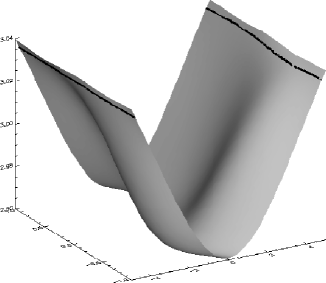
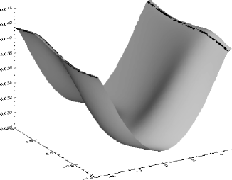
Figure 9: The proper time $\tau$ (left) and the lapse $N$ (right) in harmonic gauge with $\mathcal{J}$ freezing. The extremal values are $\tau_{\mbox{min}}=1.831$, $\tau_{\mbox{max}}=2.988$ and $N_{\mbox{min}}=0.315$, $N_{\mbox{max}}=1.151$. The black contours show the locations of the two $\mathcal{J}$’s.

In Fig. 9 we show the proper time and the lapse function for a run with harmonic gauge and scri freezing. The initial location of $\mathcal{J}$ was on the boundary $v_{0}=\pm 5$. The length of coordinate time spent was $t_{1}-t_{0}=25$ with roughly 1000 time steps. $\mathcal{J}$ has moved during this evolution at most over 3 grid points. This is due to numerical inaccuracies. We see from the figures that the evolution is much more homogeneous over the interior with differences in proper time within the interval $\left[2.96,3.04\right]$. But we also see that the lapse has decreased rapidly, from a maximum value of $0.316$ at the beginning to a maximum value of $0.0422$ in the end.

5 Mass loss and radiation

The main motivation to consider the conformal field equations in the first place is the claim that having $\mathcal{J}$ at finite places allows a well defined numerical description of the asymptotic properties like the radiative information (such as shear and news on $\mathcal{J}$) and also the global properties like the Bondi energy-momentum and angular momentum. From the nature of the hyperboloidal initial value problem it is clear that we cannot get our hands on the ADM quantities which are located at space-like infinity $i^{0}$ which is not in the domain of dependence of any hyperboloidal initial surface.

In the numerical treatment there exists a natural foliation of $\mathcal{J}$ into two-dimensional cross sections or “cuts” which is obtained from the intersection of $\mathcal{J}$ with the constant time hypersurfaces. The news, shear and the “null datum” are local quantities in the sense that their value at a point on $\mathcal{J}$ is constructed from the values of the field variables at that point. Therefore, these quantities are not sensitive to the topology of the “cuts”. In contrast, the Bondi quantities are global concepts and there is currently no way to determine their value from only local information. As a consequence they are very sensitive to the topology of the cuts and, in fact, they are so sensitive that in our case study with “cuts” which have a toroidal topology there does not exist an energy-momentum four-vector but only one scalar quantity which we still call the Bondi mass. The reason behind this unexpected phenomenon will be discussed below.

The main problem one is faced with when trying to obtain expressions for the asymptotic quantities is the fact that $\mathcal{J}$ does not look the way it does in the analytical treatments. In particular, there one usually assumes that a conformal gauge has been chosen so that $\mathcal{J}$ is divergence free, i.e., that the area of a cut does not change when the cut is moved along the null generators of $\mathcal{J}$. Since $\mathcal{J}$ itself is shear free this implies that the shape of a cut does not change either along $\mathcal{J}$ and this fact can be exploited to choose the metric on that family of cuts to be one with constant curvature. Usually this is the unit sphere metric. In our case, where the cuts have toroidal topology one would choose a flat metric on the cuts.

In a numerical treatment where the conformal factor $\Omega$ is one of the evolving variables one has almost no control of its behaviour (at least at present). Thus, we do not have the freedom to specify that $\mathcal{J}$ should have these nice properties and have to live with the way it emerges from the numerical computation. The only way to possibly influence the behaviour of the conformal factor is by way of tuning the gauge source function $\Lambda$ for the conformal gauge. However, this is a rather indirect way and at the moment it is completely unclear whether (and how) one should specify $\Lambda$ so that $\mathcal{J}$ does have the desired properties.

Another point is that the radiative quantities are referred to a specific tetrad (or spin frame) on $\mathcal{J}$ which is adapted to the geometry there. Again, in the numerical treatment the tetrad is fixed by other means which implies that we need to transform from the given tetrad to the geometric tetrad in order to obtain the correct values of the asymptotic quantities. Again, it is not yet known how to impose gauge conditions so that the computed tetrad always coincides with the geometric tetrad on $\mathcal{J}$. The transformation from the numerical frame to the adapted frame is straightforward. Recall that the condition imposed on the adapted spin frame $(O^{A},I^{A})$ is [3]:

$$\nabla_{AA^{\prime}}\Omega=-AI_{A}I_{A^{\prime}}+O(\Omega).$$ (5.1)

This condition fixes the direction of the null vector $I^{A}I^{A^{\prime}}$ but says nothing about the space-like vector $O^{A}I^{A^{\prime}}$ and its complex conjugate. Given a cut of $\mathcal{J}$ these are required to be tangent vectors to the cut. Then the transformed spin frame is fixed up to the scalings $O^{A}\mapsto c\cdot O^{A},I^{A}\mapsto c^{-1}\cdot I^{A}$. The transformation to the new spin frame is

$$O^{A} =ao^{A}+b\iota^{A},$$ (5.2)

$$I^{A} =\frac{1}{a\bar{a}+b\bar{b}}(-\bar{b}o^{A}+\bar{a}\iota^{A}),$$ (5.3)

with $a=-c\frac{2\Sigma_{22}}{\Sigma}$ and $b=c\left(\frac{2\Sigma_{21}}{\Sigma}-1\right)$ and $c$ an arbitrary complex function on the cut. With this choice of $a$ and $b$ we have achieved that on $\mathcal{J}$ the null vector $I^{A}I^{A^{\prime}}$ is aligned with the null generators of $\mathcal{J}$. The factor $A$ in (5.1) is found to be

$$A=4{c\bar{c}}\left(\Sigma_{21}-\frac{1}{2}\Sigma\right),$$ (5.4)

and we furthermore fix $c=\frac{1}{2}$ for the remainder of this section.

The asymptotic quantities with respect to the adapted frame can now be expressed on $\mathcal{J}$ in terms of the field variables. These expressions are rather lengthy in the general case but quite manageable in the symmetry reduced case that we are looking at here. Following is a list of the variables which are of interest to us and the expressions to compute them in terms of the field variables in the reduced case:

$$\sigma^{\prime} =0,\quad\kappa^{\prime}=0,$$ (5.5)

$$\rho^{\prime} =-\frac{2S}{\Sigma},\quad\tau^{\prime}=-\frac{Ss_{20}}{\Sigma}$$ (5.6)

$$\sigma =-\frac{1}{8}\left(K_{40}s_{22}^{4}+K_{44}+6K_{42}s_{22}^{2}\right)$$ (5.7)

$$\psi_{2} =\frac{1}{4}\left(E_{0}s_{22}^{2}-2E_{2}+E_{4}s_{20}^{2}\right),$$ (5.8)

$$\psi_{4} =E_{4}s_{20}^{4}+4\,B_{3}s_{20}^{3}+6\,E_{2}s_{20}^{2}+4\,B_{1}s_{20}+E_{0},$$ (5.9)

$$\mathcal{N} =\frac{1}{4}\left(\phi_{44}s_{20}^{4}+6\phi_{42}s_{20}^{2}+\phi_{40}\right)$$ (5.10)

where we have introduced $s_{22}=\frac{2\Sigma_{22}}{\Sigma}$ and $s_{20}=\frac{2\Sigma_{20}}{\Sigma}$. The function $\mathcal{N}$ is the so called “news” function.

Having these expressions at hand it is in principle straightforward to obtain the asymptotic quantities from the numerical data. The only obstacle is that the level sets of $\Omega$ do not necessarily agree with grid lines so that one has to trace out the zero set of $\Omega$ within the grid and then interpolate for the values of the field variables there. This task is greatly simplified by using the $\mathcal{J}$ fixing shift gauge discussed in section 4 when it is possible to align $\mathcal{J}$ on a grid-line initially.

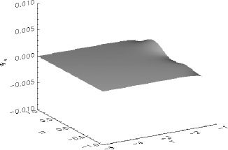
Figure 10: The “null datum” for the A3 solution.

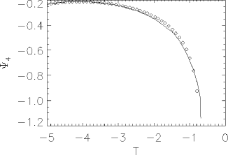
Figure 11: Time profile of $\psi_{4}$ for the W1 solution at a constant value of $u$.

In Fig. 10 we present a surface representation of the null datum $\psi_{4}$ for the A3 solution. This is a non-radiating solution so $\psi_{4}$ should vanish. Indeed, we find that only when the singularity is approached the function differs significantly from zero. This is due to the closeness of the singularity. We should also point out that this figure has been produced in the warped coordinate system without the use of the $\mathcal{J}$ fixing shift gauge. It is only in the late stages and in the central region where the warping is maximal when the tracing out of $\mathcal{J}$ produces too large errors. In a similar way the W1 solution was treated. Now, $\psi_{4}$ cannot be expected to vanish because this is a radiating solution. Since there is an additional symmetry present in the solution which is aligned along $\mathcal{J}$ the function should be constant on $\mathcal{J}$. We found that the tracing algorithm works quite satisfactorily in this case also in that the computed $\psi_{4}$ is indeed constant as a function of the $u$-coordinate along $\mathcal{J}$. Therefore, we show in Fig. 11 only a time profile for constant $u$. The line indicates the exact function while the markers indicate the computed values. The relative error in this calculation (200 by 200 points) is a few percent in the region where the influence of the singularity is not too strong.

Let us now discuss some of the issues related to the Bondi energy-momentum. This is an unexpectedly complicated issue which, in addition, depends on the global topology of the space-time under consideration. The standard definition used here is from [3]:

$$m_{B}\left[W\right]=\oint_{C}\left\{\psi_{2}-\frac{\sigma\mathcal{N}}{A}\right\}W\;d^{2}\mathcal{S},$$ (5.11)

where the integration is over a cut of $\mathcal{J}$. As it stands the formula is only valid under rather stringent simplifying assumptions. It is assumed that the surfaces $\Omega=\mathrm{const}$ are null even away from $\mathcal{J}$. This implies that $\mathcal{J}$ is non diverging and that the spin-coefficient $\tau^{\prime}$ vanishes. If these assumptions are not made, then the news $\mathcal{N}$ acquires additional compensating terms.

The function $W$ which appears in (5.11) is a function with conformal weight $+1$ on the cut satisfying the conformally invariant second order elliptic equation

$$\eth_{c}^{2}W=0.$$ (5.12)

Here, the $\eth_{c}$ is the conformally invariant “eth” operator introduced in [3]. For a more standard form of this equation, we refer to [11]. The purpose of solving the equation (5.12) is to select out of the super-translation subgroup of the asymptotic symmetry group (the BMS group) the normal subgroup of translations which is used to generate the energy-momentum. In the special case, where the metric on the cut has been scaled to be the standard unit sphere metric and where the cut sits within $\mathcal{J}$ in such a way that the spin-coefficient $\tau$ vanishes, then the equation (5.12) has four linearly independent solutions which can be taken as the first four spherical harmonics $Y_{lm},\;l=0,1$. Note, that $\tau=0$ can always be achieved in the neighbourhood of a single cut, because it only involves parallel transport of $O^{A}$ along the null generators. However, given a system of cuts and an adapted spin frame, this condition cannot, in general, be maintained. Unfortunately, this is the case for the cuts appearing in the numerical treatment as intersections of $\mathcal{J}$ with the constant time hypersurfaces. A more thorough discussion of the general spherical case is left to another paper.

Here we want to focus on our immediate interest, namely obtaining a formula for the Bondi mass on cuts with toroidal topology. In that case, the BMS group has a completely different structure. This is reflected in the fact that equation (5.12) on a torus has only a one dimensional solution space as opposed to the four dimensions in the spherical case. This means that the translation subgroup is a one-dimensional subgroup of the BMS group. Therefore, on toroidal cuts, there does not exist a four-vector of energy-momentum, but only a “Bondi scalar”, which we call the Bondi mass.

In order to compare the evolution of that scalar with time in our special case we observe that for the initial data obtained from the exact solutions A3 and W1, the cuts are spanned by Killing vectors. This implies that on the cut all field variables are constant. Hence, we may take $W=\mathrm{const}$ as a solution of (5.12) and since $W$ has to be a conformal density of weight $+1$ we take $W=\sqrt{\mathcal{A}}$, with $\mathcal{A}$ being the area of the cut. Thus, we end up with the formula

$$m_{B}=-\sqrt{\mathcal{A}}\oint_{C}\left\{\psi_{2}-\frac{\sigma}{A}\left(\mathcal{N}-\bar{\sigma}\rho^{\prime}\right)\right\}\;d^{2}\mathcal{S}.$$ (5.13)

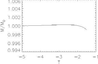
Figure 12: The Bondi mass for the A3 solution normalised against its initial value.

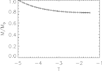
Figure 13: The Bondi mass for the W1 solution normalised against its initial value.

Of course, due to the constancy of the integrand on the cut we could have written this formula without the integral. However, we implement the formula with the integral because it averages over the numerical inaccuracies present from the interpolation process. In Fig. 12 is shown the (normalised) Bondi-mass for the A3 solution, which of course should remain constant. Similarly, Fig. 13 presents the Bondi mass for the W1 solution. Again, the solid line is the exact profile while the markers are the values obtained from the numerical solution.

6 Conclusion

In this article we have presented and discussed several issues concerning the numerical solution of the evolution part of the hyperboloidal initial value problem for the vacuum conformal field equations. We have described a special case where the unphysical assumption was made that there exists a hypersurface orthogonal Killing vector with closed orbits and no fixed points. This does not alter the essential issues. The numerical evolution scheme is a simple two-dimensional implementation of the well-known Lax-Wendroff method. The outer boundary is evolved using a stable eigen-field method. We have discussed various lapse choices and the features which appear when one specifies the gauge source function $F$ as a function of the field variables. We have found a special choice for the shift vector which originates in the conformal properties of the system. This shift allows us to freeze null infinity on the grid while still leaving the usual freedom for specifying a shift vector in the interior. Finally, we have described how to obtain the local radiative information by simply “reading it off” $\mathcal{J}$ and transforming to the appropriate asymptotic spin frame. The global quantities like Bondi four-momentum are more difficult to determine and they are very different in our present case from the physical case where $\mathcal{J}$ has spherical sections. We have tested the code and the radiation extraction algorithm using exact solutions. We obtained good agreement between the analytical and the numerical solution. Unfortunately, the used exact solutions have an additional Killing vector which makes them rather special even though we try to compensate for this by “warping” the coordinate system. Naturally, the next step has to be to obtain more general initial data.

Appendix A The exact solutions

We have used several exact solutions for numerical tests. Apart from the trivial ones which are simply Minkowski space in disguise, i.e., rescaled with an arbitrary conformal factor there is the class of vacuum space-times with toroidal null infinities which have been constructed by Schmidt [2] for exactly that purpose. They are characterised by a solution $w$ of a two-dimensional wave equation and are defined as follows

$$\Omega =\frac{1}{8}\left(t^{2}-z^{2}\right)$$ (A.1)

$$g =\frac{e^{2n(t,z)}}{\sqrt{t^{2}+z^{2}}}\left(d\,t^{2}-d\,z^{2}\right)-\left(t^{2}+z^{2}\right)\left(e^{2w(t,z)}d\,x^{2}+e^{-2w(t,z)}d\,y^{2}\right).$$ (A.2)

Given a solution of the two-dimensional wave equation [12]

$$\left(t^{4}-z^{4}\right)\left(w_{tt}-w_{zz}\right)-2t\left(3z^{2}+t^{2}\right)\,w_{t}-2z\left(3t^{2}+z^{2}\right)\,w_{z}=0,$$ (A.3)

one can obtain the function $n(t,z)$ by quadratures. The coordinates $x$ and $y$ are Killing coordinates, each taking values in $\mathbf{R}$. We identify the points $(x,y)$ and $(x+1,y+r)$ to obtain the toroidal topology. In our applications, we always have $r=1$. The simplest solutions of this type are the ones obtained by choosing $w(t,z)=0$ (with $n(t,z)=0$) and $w(t,z)=A(t^{2}-v^{2})$ for some constant $a$ (with $n(t,z)=-\frac{1}{2}A^{2}(t^{2}+z^{2})^{2}$). Note, that $A=0$ in the latter solution gives the former. The physical metric which corresponds to the first of these appears in the classification by Ehlers and Kundt [13] under the name A3 as the analogue of the Schwarzschild metric in plane symmetry. Here are the explicit expressions for the variables we use in the code.

$$N =\frac{1}{\sqrt{2}}\,{\frac{1}{\sqrt[4]{U}}}{e^{-\frac{1}{2}\,{A}^{2}U^{2}}}, K =\frac{t}{\sqrt{2}}\,\frac{\left(4\,{A}^{2}U^{2}-3\right)}{U^{3/4}}{e^{\frac{1}{2}\,{A}^{2}U^{2}}},$$

$${C_{31}} =\frac{1}{\sqrt{2}}\,{\frac{1}{\sqrt{U}}}{e^{-A\left(t^{2}-v^{2}\right)}}, {K_{20}} =-i\frac{v}{\sqrt{2}}\,{\frac{4\,U^{2}{A}^{2}+1}{U^{3/4}}}\,{e^{\frac{1}{2}\,{A}^{2}U^{2}}},$$

$${C_{10}} =\frac{1}{\sqrt{2}}\,{\frac{1}{\sqrt{U}}}e^{A\left(t^{2}-v^{2}\right)}, {K_{40}} =\frac{t}{2\sqrt{2}}\,{\frac{4\,{A}^{2}U^{2}+4\,AU+3}{U^{3/4}}}\,{e^{\frac{1}{2}\,{A}^{2}U^{2}}},$$

$${C_{20}} =\frac{i}{\sqrt{2}}\,\sqrt[4]{U}{e^{\frac{1}{2}\,{A}^{2}U^{2}}}, {K_{42}} =\frac{t}{6\sqrt{2}}\,{\frac{4\,{A}^{2}U^{2}-12\,AU+3}{U^{3/4}}}\,{e^{\frac{1}{2}\,{A}^{2}U^{2}}},$$

$${\gamma_{20}} =i\frac{v}{\sqrt{2}}\,{\frac{1}{U^{3/4}}}\,{e^{\frac{1}{2}\,{A}^{2}U^{2}}}, {\phi_{42}} =\frac{1}{6}\,{\frac{4\,{A}^{2}U^{2}-12\,AU+1}{\sqrt{U}}}\,{e^{{A}^{2}U^{2}}},$$

$${\gamma_{41}} =-i\frac{v}{\sqrt{2}}\,\sqrt[4]{U}A{e^{\frac{1}{2}\,{A}^{2}U^{2}}}, {\phi_{40}} =\frac{1}{2}{\frac{4\,{A}^{2}U^{2}+4\,AU+1}{\sqrt{U}}}\,{e^{{A}^{2}U^{2}}},$$

$$F =4\,{\frac{t}{\sqrt{U}}}\,{e^{{A}^{2}U^{2}}}. {E0} =-2\,{\frac{8\,U^{3}{A}^{3}+12\,{A}^{2}U^{2}+6\,AU-3}{U^{3/2}}}\,{e^{{A}^{2}U^{2}}},$$

$$S =\frac{1}{4}\,{e^{{A}^{2}U^{2}}}\sqrt{U}, {E2} =2\,{\frac{8\,U^{3}{A}^{3}-4\,{A}^{2}U^{2}+6\,AU+1}{U^{3/2}}}\,{e^{{A}^{2}U^{2}}},$$

$$\Sigma =\frac{1}{2\sqrt{2}}\,t\sqrt[4]{U}{e^{\frac{1}{2}\,{A}^{2}U^{2}}}, \phi =-2\,{\frac{4\,{A}^{2}U^{2}+1}{\sqrt{U}}}\,{e^{{A}^{2}U^{2}}},$$

$${\Sigma_{20}} =-i\frac{v}{2\sqrt{2}}\,\sqrt[4]{U}{e^{\frac{1}{2}\,{A}^{2}U^{2}}},$$

with $U=t^{2}+z^{2}$. All other functions either vanish or they are complex conjugates of functions given above.

Figures

References

- [1] J. Frauendiener. Numerical treatment of the hyperboloidal initial value problem for the vacuum Einstein equations. I. The conformal field equations. preprint.
- [2] B. G. Schmidt. Vacuum space-times with toroidal null infinities. Class. Quant. Grav., 13, p. 2811–2816, 1996.
- [3] R. Penrose and W. Rindler. Spinors and Spacetime, volume 2. Cambridge University Press, 1986.
- [4] R. McLenaghan. NP: A Maple package for performing calculations in the Newman-Penrose formalism. Gen. Rel. Grav., 19, p. 623–635, 1987.
- [5] R. Courant, K. O. Friedrichs, and H. Lewy. Über die partiellen Differenzengleichungen der mathematischen Physik. Math. Ann, 100, p. 32–74, 1928.
- [6] H. O. Kreiss. Stability theory for difference approximations of mixed initial boundary value problems. I. Math. Comp., 22, p. 703–714, 1968.
- [7] B. Gustafsson, H. O. Kreiss, and A. Sundström. Stability theory for difference approximations of mixed initial boundary value problems. II. Math. Comp., 26, p. 649–686, 1972.
- [8] L. N. Trefethen. Group velocity in finite difference schemes. SIAM Review, 24, p. 113–136, 1982.
- [9] H. Friedrich and G. Nagy. The initial boundary value problem for Einstein’s vacuum field equations. preprint, 1998.
- [10] R. J. LeVeque. Wave propagation algorithms for multidimensional hyperbolic systems. J. Comp. Phys., 131, p. 327–353, 1997.
- [11] R. Geroch. Asymptotic structure of space-time. In F. P. Esposito and L. Witten, editors, Asymptotic structure of space-time. Plenum, New York, 1977.
- [12] P. Hübner. More about Vacuum Spacetimes with Toroidal Null Infinities. unpublished, 1997.
- [13] J. Ehlers and W. Kundt. Exact solutions of the gravitational field equations. In L. Witten, editor, Gravitation: an introduction to current research. J. Wiley, New York, 1962.