ACT-19/97

CTP-TAMU-50/97

NTUA-68/97

OUTP-97-69P

UA-NPPS-9-97

December 1997

gr-qc/9712051

Irreversible Time Flow in a Two-Dimensional Dilaton Black Hole with Matter
G.A. Diamandis^a,∗, John Ellis^b, B.C. Georgalas^a,∗ N.E. Mavromatos^a,
D.V. Nanopoulos^c, and E. Papantonopoulos^d
Abstract
We show that an exact solution of two-dimensional dilaton gravity with matter discovered previously exhibits an irreversible temporal flow towards flat space with a vanishing cosmological constant. This time flow is induced by the back reaction of matter on the space-time geometry. We demonstrate that the system is not in equilibrium if the cosmological constant is non-zero, whereas the solution with zero cosmological constant is stable. The flow of the system towards this stable end-point is derived from the renormalization-group flow of the Zamolodchikov function. This behaviour is interpreted in terms of non-critical Liouville string, with the Liouville field identified as the target time.

^a University of Oxford, Dept. of Physics (Theoretical Physics), 1 Keble Road, Oxford OX1 3NP, United Kingdom

^b Theory Division, CERN, CH-1211 Geneva, Switzerland

^c Center for Theoretical Physics, Dept. of Physics, Texas A & M University, College Station, TX 77843-4242, USA, Astroparticle Physics Group, Houston Advanced Research Center (HARC), The Mitchell Campus, Woodlands, TX 77381, USA, and Academy of Athens, Chair of Theoretical Physics, 28 Panepistimiou Ave., Athens GR-10679, Greece.

^d Physics Department, National Technical University, Zografou GR-157 80, Athens, Greece,

^∗ On leave from Nuclear and Particle Physics Section, Physics Department, Athens University, Panepistimiopolis, Athens GR-157 71, Greece.

1 Introduction

Two-dimensional black holes [1, 2, 3] are a useful laboratory for studying fundamental issues of quantum gravity, such as the structure of black-hole space times and the information paradox. One of their most useful features is their exact solubility. Moreover, despite their two-dimensional nature, these black holes exhibit many of the interesting and non-trivial features of their higher-dimensional counterparts, namely horizons related to the exponential of the dilaton field, Hawking radiation [7, 6], non-thermal back reaction effects [8], etc.. Recently, many of the features found previously in two-dimensional stringy black-hole models have been recovered in the $D$-brane description of black holes in higher-dimensional space times.

The two-dimensional stringy black hole has also served as a prototype system for developing the interpretation of the world-sheet Liouville field as a target-space temporal evolution parameter [9, 10, 11]. The propagating light matter modes  of the two-dimensional stringy black hole exhibit non-trivial conformal dynamics due to their coupling with discrete quasi-topological higher-level modes, which constitute an ‘environment’ that is not observable in conventional low-energy scattering experiments [9]. These modes are therefore integrated out in the effective low-energy theory of the light modes, which exhibits coherence loss due to this entanglement with the higher-level modes. It has been argued [12] on the basis of a general renormalization-group analysis and explicit $D$-brane examples that these features are shared by more realistic string models in higher dimensions.

In this paper we investigate these arguments using an exact solution of two-dimensional dilaton gravity with matter which some of us have discovered previously. We argue here that it presents features suggested in the approach of [9, 11]. In particular, the Liouville field may be identified as the target time-evolution parameter in the two-dimensional dilaton-gravity-matter system. This two-dimensional black-hole space time features infalling matter and a non-zero cosmological constant. It is unstable, and is interpreted as an time-dependent non-equilibrium black hole, which exhibits a potential flow towards a flat space time with a zero comsological constant, which is stable.

Our first demonstration of the instability of the solution with non-zero cosmological solution is made by evaluating the coefficients of the Bogolubov transformation between the asymptotic ‘in’ and ‘out’ states. These yield particle creation with a number density that deviates from a thermal equilibrium distribution, if the cosmological constant is non-zero. On the other hand, there is no particle production in the limit of zero cosmological constant. We then show how these results can be interpreted in the context of Zamolodchikov’s $c$ theorem as flow towards a fixed point of the renormalization group, exhibiting explicitly the rate of this flow in the weak-field approximation. This analysis is based on the identification [9, 11, 10] of the (world-sheet) renormalization scale, i.e., the renormalization-group evolution parameter, with the world-sheet Liouville field and the target time variable.

2 Review of the Two-Dimensional Dilaton Black Hole with Matter

For completeness, we first review relevant aspects of the dilaton-matter black-hole solution found in [5]. In two dimensions, the action of the dilaton-tachyon system coupled to gravity is

$$S=\frac{1}{2\pi}\int d^{2}x\sqrt{-g}\{e^{-2\phi}[R+4(\nabla\phi)^{2}-(\nabla T)^{2}-V(T)+4\lambda^{2}]\}$$ (1)

where $4\lambda^{2}$ is the two-dimensional cosmological constant, which is related to the central charge $c$ of the corresponding world-sheet $\sigma$ model via [1]:

$$\lambda^{2}=\frac{k}{3}(c-26)$$ (2)

where $k>2$ is the level parameter of the Wess-Zumino conformal field theory that has as a conformal solution the target-space two-dimensional theory (1), which is in turn related to the central charge by [1] $c=(3k/k-2)-1$. The quantity $V(T)$ is the tachyon potential, which is ambiguous in string theory [13]. The only unambiguous term is the quadratic term for the tachyon field, which is also all that we need for our analysis. The equations of motion resulting from the action (1), which are equivalent at ${\cal O}(\alpha^{\prime})$ to the conformal-invariance conditions of the $\sigma$ model, are

$$\Box\phi-(\nabla\phi)^{2}+\frac{1}{4}R-\frac{1}{4}(\nabla T)^{2}+\frac{1}{2}T^{2}+\lambda^{2}=0$$ (3)

$$\Box T-2(\nabla\phi)(\nabla T)+2T=0$$

$$\Box\phi-2(\nabla\phi)^{2}+T^{2}+2\lambda^{2}=0$$

These equations can be analyzed most easily in the conformal gauge

$$g_{\mu\nu}=e^{2\rho}n_{\mu\nu}\quad,\quad n_{\mu\nu}=diag(-1,1)$$

and if we use light-cone coordinates $x^{\pm}=x^{0}\pm x^{1}$. From now on, we shall refer to $\rho$ as the conformal factor, and we shall follow [9] by identifying it with the Liouville field.

An exact solution of this model with a non-trivial time-dependent tachyon configuration was found in [5], by assuming that the tachyon $T$ is a function of $x^{+}$.  The following solution to the system of equations (3) was obtained in [5]:

$$e^{-2\phi}=e^{-2\rho}=C_{1}F(1,\frac{\lambda^{2}}{2}+1;-\frac{T^{2}}{4})+C_{2}(\frac{T^{2}}{4})^{-\frac{\lambda^{2}}{2}}e^{-\frac{T^{2}}{4}}-\frac{2e^{-\frac{T^{2}}{4}}}{a(T^{2})^{\frac{\lambda^{2}}{2}}}x^{-}$$ (4)

where $F(\alpha,\beta;c)$ is the confluent hypergeometric function, and $a>0$, $C_{1}>0$ and $C_{2}$ are integration constants. The solution has been expressed in terms of the tachyon field, which satisfies:

$$\frac{dT^{2}}{dx^{+}}=-a(T^{2})^{\frac{\lambda^{2}}{2}+1}e^{\frac{T^{2}}{4}}$$ (5)

The parametrization in terms of the tachyon field was made possible by the monotonic behaviour of the field $T$, which admits the physical interpretation of the tachyon field $T$ as an infalling matter field. The relation (5) can be integrated in a closed form to give:

$$x^{+}=\frac{1}{4^{\frac{\lambda^{2}}{2}}a}\Gamma(-\frac{\lambda^{2}}{2},\frac{T^{2}}{4})$$ (6)

where $\Gamma(\alpha,\beta)$ denotes the incomplete Gamma function [14]. The asymptotic behaviour of the matter field is such that at $x^{+}\rightarrow\infty(0)$ the matter background $T^{2}\rightarrow 0(\infty)$. For later use, we also present here an expression for the curvature scalar, which in two dimensions determines completely the Riemann tensor:

$$R=\frac{4\lambda^{2}C_{1}}{C_{1}F(1,\frac{\lambda^{2}}{2}+1;-\frac{T^{2}}{4})+C_{2}(\frac{T^{2}}{4})^{-\frac{\lambda^{2}}{2}}e^{-\frac{T^{2}}{4}}-\frac{2e^{-\frac{T^{2}}{4}}}{a(T^{2})^{\frac{\lambda^{2}}{2}}}x^{-}}$$ (7)

We see immediately that in this model one obtains a flat space time if the cosmological constant $\lambda^{2}$ vanishes, provided one stays away from the initial singularity at $x^{+}=0$, where the tachyon field diverges. 

For general $\lambda^{2}\neq 0$, i.e., central charges $c\neq 26$, as seen in (2), the above solution has the structure of a non-static time-dependent black hole, with the important feature [5] that there is a tachyon singularity at $x^{+}=0$, which is displayed in Fig. 1. Thus there is no white hole in this model, which we find suggestive that the model may exhibit an arrow of time.

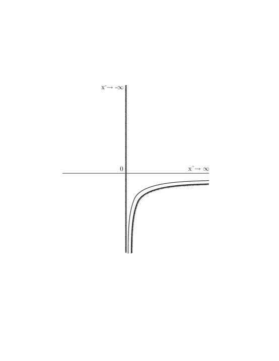
Figure 1: The non-static solution of the equations of motion corresponding to an infalling matter $T=T(x^{+})$. The singularities are indicated by jagged lines, and the apparent horizon is represented by the thin continuous line. It is clear that there is no white hole.

3 Analysis of Stability and Particle Production

Motivated by this indication of a possible arrow of time in this model, we now look for a connection with the irreversible Liouville time flow along the lines suggested in [9, 10]. The first step in this search is to find a coordinate transformation which makes the Liouville mode, i.e., the conformal factor $\rho$ in the metric (4), linear in the transformed time variable. As we discuss below, this is possible only when the cosmological constant $\lambda^{2}=0$, corresponding (2) to a critical value for the central charge, and representing a stable, equilibrium configuration. For the other values of $\lambda^{2}>0$, the conformal factor also has a spatial dependence, as we also discuss below.

3.1 The $\lambda=0$ Case: Stability

We first examine the structure of the solution at the point $\lambda^{2}=0$, corresponding to $c=26$, where the space time is flat (7). In this case, the metric simplifies to:

$$e^{-2\phi}=e^{-2\rho}=[(C_{1}+C_{2})-\frac{2}{a}x^{-}]e^{-\frac{T^{2}}{4}}$$ (8)

Setting $C_{1}=-C_{2}$ by making a shift in $x^{-}$, the metric corresponding to (8) becomes:

$$ds^{2}=\frac{a}{2}\frac{e^{\frac{T^{2}}{4}}}{x^{-}}dx^{+}dx^{-}$$ (9)

where the tachyon field $T$ obeys the equation

$$\frac{dT^{2}}{dx^{+}}=-aT^{2}e^{T^{2}/4}$$ (10)

We can use (10) to recast (9) in the form:

$$ds^{2}=-\frac{1}{2}\frac{dT^{2}dx^{-}}{T^{2}x^{-}}$$ (11)

which is the basis for further discussion of the structure of this solution.

In order to establish a connection between the dilaton and the target time variable, we first consider the coordinate transformation $x^{\pm}\rightarrow(r^{\prime},t^{\prime})$ with

$$r^{\prime}={\rm ln}(-y^{+}y^{-}),\qquad t^{\prime}=-{\rm ln}(-\frac{y^{-}}{y^{+}})$$ (12)

where $y^{\pm}$ are the corresponding Kruskal-Szekeres coordinates:

$$T^{2}=\frac{1}{y^{+}},\qquad,\qquad x^{-}=y^{-}$$ (13)

In this coordinate system, the matter background (13) is singular at $y^{+}=0$, whilst the metric element becomes that of Minkowski space time. The background dilaton has the form

$$\phi=\frac{1}{2}{\rm ln}(a/2)+\frac{t^{\prime}-r^{\prime}}{4}+\frac{1}{8}e^{-(r^{\prime}+t^{\prime})/2}$$ (14)

which has the asymptotic behaviour: $\phi\rightarrow-r^{\prime}/4$, as $r^{\prime}\rightarrow\infty$ for $t^{\prime}$ finite, and $\phi\rightarrow t^{\prime}/4$ as $t^{\prime}\rightarrow\infty$ for $r^{\prime}$ finite. Thus the dilaton may have a linear asymptotic dependence on time [16, 9], in the presence of non-trivial matter.

The above representation is not convenient for deriving tractable closed-form expressions, for which purpose it is better to consider an alternative coordinate transformation $x^{\pm}\rightarrow(r,t)$ where

$$r={\rm ln}(-{\tilde{x}}^{+}{\tilde{x}}^{-}),\qquad t=-{\rm ln}(-\frac{{\tilde{x}}^{-}}{{\tilde{x}}^{+}})$$ (15)

so that ${\tilde{x}}^{\pm}$ are a new pair of Kruskal-Szekeres coordinates. We define ${\tilde{x}}^{-}\equiv x^{-}$ and

$$({\tilde{x}}^{+})^{2}\equiv-{\rm ln}({T^{2}\over\beta})$$ (16)

The validity of this coordinate transformation follows from the monotonic behaviour of the tachyon solution. We shall use (16) as a coordinate patch when $T^{2}\leq\beta$, i.e., when ${\tilde{x}}^{+}\geq 0$. The parameter $\beta$ can be regarded as ‘brick-wall’ cut-off that shields the matter singularity that appears when $y^{+}=0$ in the previous coordinate system. After the transformation (16), the metric element becomes:

$$ds^{2}=-\left(-\frac{{\tilde{x}}^{+}}{{\tilde{x}}^{-}}\right)d{\tilde{x}}^{+}d{\tilde{x}}^{-}=\frac{1}{4}e^{(r+t)}(-dt^{2}+dr^{2})$$ (17)

and the conformal factor $\rho$ becomes a simple linear function of time:

$$\rho=\frac{t}{2}$$ (18)

The dilaton background, however, still depends on both $(r,t)$:

$$\phi=\frac{1}{2}{\rm ln}(a/2)+\frac{t-r}{4}+\frac{\beta}{8}{\rm exp}[-e^{r+t}]$$ (19)

with the linear asymptotic behaviours: $\phi\rightarrow-r/4$, as $r\rightarrow\infty$ for $t$ finite, and $\phi\rightarrow t/4$ as $t\rightarrow\infty$ for $r$ finite.

The physical interpretation of the metric (17) becomes transparent in terms of the following variables:

$$\xi\equiv e^{r/2}\qquad;\qquad\tau=t/2$$ (20)

Looking at the metric element as a function of ($\xi,\tau$):

$$ds^{2}=e^{2\tau}\left(-\xi^{2}d\tau^{2}+d\xi^{2}\right)$$ (21)

we see that the space is conformally equivalent to a two-dimensional Rindler space with constant acceleration [17].  We notice also the appearance of a conformal factor $e^{2\tau}=e^{t}$ corresponding to an expanding universe. This suggests an alternative representation in terms of the following variables:

$$\eta\equiv e^{t/2}\qquad;\qquad r^{\prime}=r/2$$ (22)

which maps (21) into a two-dimensional Universe that is conformally equivalent to a Milne space-time [17], but with a conformal factor that depends only on space:

$$ds^{2}=e^{2r^{\prime}}\left(-d\eta^{2}+\eta^{2}dr^{{}^{\prime}2}\right)$$ (23)

It is known [17] that both Rindler and Milne spaces exhibit particle creation, related to the cosmological expansion. The peculiarity of our metric (21) or equivalently (23) resides in the fact that it constitutes a mixing of the two, and hence one has to reconsider the analysis of particle production for this case.

For this purpose, we now compute the Bogolubov coefficients corresponding to the metric (17). This may conveniently be achieved by the following coordinate transformation:

$$\xi^{\prime}\equiv\frac{1}{4}e^{2(r+t)}+\frac{1}{4}(r-t)$$ (24)

$$\eta^{\prime}\equiv\frac{1}{4}e^{2(r+t)}-\frac{1}{4}(r-t)$$

where $\eta^{\prime}$ may be regarded as a time variable. The space parametrized by these $(\xi^{\prime},\eta^{\prime})$ variables is considered as the ‘out’ space, with the ‘in’ space characterized by the metric (17). The Bogolubov transformations [17] are given in the usual way by:

$$\alpha=<\Phi^{out}|\Phi^{in}>=\int dr\left(u^{in*}\partial_{t}u^{out}-\partial_{t}u^{in*}u^{out}\right)$$ (25)

$$|\alpha|^{2}-|\beta|^{2}=1$$

where

$$\Phi^{out}=\alpha\Phi^{in}+\beta\Phi^{out*}$$ (26)

and the $\beta$ coefficient is associated with particle creation. It is straightforward to see that in our case:

$$\alpha=1\qquad;\qquad\beta=0$$ (27)

independently of the mode energies and momenta. Thus, there is no particle production in this metric.

This means that the model with $\lambda=0$ is a stable equilibrium state. Perhaps surprisingly, the effects of the spatial expansion visible in (21) and the Rindlerlike acceleration [18] cancel exactly, as far as particle production is concerned.

3.2 The $\lambda\neq 0$ Case: Instability

The same is not the case in the case $\lambda^{2}\neq 0$, as we discuss now. From the point of view of the target-space theory (1), this case corresponds to a time-dependent black-hole solution [5]. We would therefore expect that it corresponds to a non-equilibrium situation, since the non-trivial time dependence means that a temperature cannot be defined for the system. To demonstrate this explicitly, we compute the Bogolubov coefficients of the vacuum described by the $\lambda\neq 0$ model, and then the corresponding particle creation number seen by an observer who initially observes a flat space time at $t\rightarrow-\infty$.

The line element in this case is given by (4). For simplicity, we consider the case with weak matter fields $|T|<<1$, such that

$$\frac{\lambda^{2}}{2}|{\rm ln}(\frac{T^{2}}{4})|<<1$$ (28)

For convenience, and without loss of generality, we take $C_{1}=-C_{2}$. The line element can then be approximated by:

$$ds^{2}=\frac{\frac{dT^{2}}{T^{2}}dx^{-}}{a4^{\frac{\lambda^{2}}{4}}C_{1}~{}\frac{\lambda^{2}}{2}~{}{\rm ln}\frac{T^{2}}{4}-2x^{-}}$$ (29)

in light-cone coordinates, where we have used (5). To facilitate our analysis, we assume both an infrared cut-off $\Lambda$ and an ultraviolet cut-off $\epsilon$ in time. The matter field $T$, defined in (5), acquires a minimum value $T^{2}(\Lambda)=T^{2}_{min}$, such that (28) is satisfied for $T=T_{min}$, and a maximum value $T^{2}_{max}-T^{2}_{min}\equiv 4{\cal B}>0$, where ${\cal B}$ a constant related to the cut-offs.

Next we define a convenient coordinate basis ${\tilde{\sigma}}^{+}$, ${\tilde{\sigma}}^{-}$ by:

$$e^{{\tilde{\sigma}}^{+}}\equiv\frac{1}{2}{\rm ln}\left(\frac{4{\cal B}}{T^{2}-T_{min}^{2}}\right)\qquad{\tilde{\sigma}}^{-}\equiv-{\rm ln}(-x^{-})$$ (30)

in terms of which the line element reads:

$$ds^{2}=\frac{-2{\cal F}({\tilde{\sigma}}^{+})e^{2{\tilde{\sigma}}^{+}-{\tilde{\sigma}}^{-}}d{\tilde{\sigma}}^{+}d{\tilde{\sigma}}^{-}}{A\frac{\lambda^{2}}{2}{\rm ln}T_{min}^{2}/4+\frac{4A(\lambda^{2}/2){\cal B}}{T_{min}^{2}}e^{-e^{2{\tilde{\sigma}}^{+}}}+2e^{-{\tilde{\sigma}}^{-}}}\qquad A=4^{\lambda^{2}/2}~{}a~{}C_{1}$$ (31)

where

$${\cal F}({\tilde{\sigma}}^{+})=(1+T_{min}^{2}{\rm exp}(e^{2{\tilde{\sigma}}^{+}})/4{\cal B})^{-1}$$ (32)

This geometry has the following asymptotic behaviour at early and late times:

$$ds^{2}_{in}=-e^{2{\tilde{\sigma}}^{+}}d{\tilde{\sigma}}^{+}d{\tilde{\sigma}}^{-},\qquad t\rightarrow-\infty$$ (33)

$$ds^{2}_{out}=-\frac{2{\cal F}({\tilde{\sigma}}^{+})}{b+2e^{-{\tilde{\sigma}}^{-}}}e^{2{\tilde{\sigma}}^{+}-{\tilde{\sigma}}^{-}}d{\tilde{\sigma}}^{+}d{\tilde{\sigma}}^{-},$$

$$b\equiv A\frac{\lambda^{2}}{2}{\rm ln}T_{min}^{2}/4+\delta>0\qquad t\rightarrow+\infty$$

where $\delta$ is related to the time cut-offs introduced earlier, and is such that the signature of the metric does not change as time flows from $-\Lambda$ to $\Lambda$.

In the ‘in’ vacuum $t\rightarrow-\infty$, the modes in terms of which a spectator scalar field should be expanded are standard Minkowski modes for right movers only, i.e., functions of $x^{-}$, as is appropriate for an incoming wave. In this construction, the matter field $T(x^{+})$ constitutes an infalling matter sector. The ‘in’ modes are therefore:

$$u_{in}=\frac{1}{\sqrt{2\omega_{1}}}e^{-i\omega_{1}\Sigma^{-}}\qquad\Sigma^{+}=\frac{1}{2}e^{2{\tilde{\sigma}}^{+}}~{};~{}\Sigma^{-}={\tilde{\sigma}}^{-}$$ (34)

On the other hand, the ‘out’ modes are defined by:

$$u_{out}=\frac{1}{\sqrt{2\omega_{2}}}e^{\pm i\omega_{2}{\rm ln}(1+\frac{2}{b}e^{-\Sigma^{-}})}$$ (35)

We notice immediately that the ‘out’ spectrum contains both positive and negative frequencies.

We focus on the positive frequency modes, which determine the particle creation number for an external observer. This is determined as usual by the Bogolubov $\beta$ coefficient [17], which in this case is easily found to be:

$$\beta_{\omega_{1}\omega_{2}}^{>0}=\frac{i}{\pi}\int_{-\infty}^{0}d\Sigma^{-}\frac{1}{\sqrt{2\omega_{2}}}e^{i\omega_{2}{\rm ln}(1+\frac{2}{b}e^{-\Sigma^{-}})}\partial_{\Sigma^{-}}\left(\frac{1}{\sqrt{2\omega_{1}}}e^{-i\omega_{1}\Sigma^{-}}\right)=$$ (36)

$$\frac{i}{2\pi(\omega_{1}+\omega_{2}+i\epsilon)}\sqrt{\frac{\omega_{1}}{\omega_{2}+i\epsilon}}\left(\frac{b}{2}\right)^{\epsilon-i(\omega_{1}+\omega_{2})}$$

$${}_{2}F_{1}(\epsilon-i(\omega_{1}+\omega_{2}),\epsilon-i\omega_{2},1-i(\omega_{1}+\omega_{2});-\frac{b}{2})$$

where $\epsilon>0$ specifies the infrared pole prescription for the frequencies, whose form is dictated by the defining properties of the integral representation of the hypergeometric function. Notice that the presence of $\epsilon$ guarantees a smooth connection with the case $b=0$, corresponding to the case with cosmological constant $\lambda=0$.

The corresponding particle number is given by;

$$N_{\omega_{2}}=\int_{0}^{\infty}d\omega_{1}|\beta_{\omega_{1}\omega_{2}}|^{2}$$ (37)

The spectrum is clearly not thermal, This can also as can be seen analytically from (36),(37) in the case of $b<<1$, where we may expand the hypergeometric function in powers of $b$.  For very small $\beta$ and low frequencies $\omega_{2}$, the leading terms in (37) have an inverse-power-law dependence on $\omega_{2}$,

$$N_{\omega_{2}}\sim\frac{1}{\omega_{2}}\int_{0}^{\Lambda}d\omega_{1}\frac{\omega_{1}}{(\omega_{1}+\omega_{2})^{2}}=\frac{1}{\omega_{2}}\left({\rm ln}\frac{\Lambda+\omega_{2}}{\omega_{2}}-\frac{\Lambda}{\Lambda+\omega_{2}}+{\cal O}(b)\right)$$ (38)

and it can easily be checked that the ${\cal O}(b)$ terms in the expansion of the hypergeometric function are finite as $\Lambda\rightarrow\infty$.

Further analytic support for a deviation from a thermal distribution comes by representing the conformal factor $\rho$ (4) in the form:

$$e^{-2\rho}= C_{1}-4^{\frac{\lambda^{2}}{2}}\frac{\lambda^{2}a}{2}C_{1}x^{+}-\lambda^{2}x^{+}x^{-}+$$ (39)

$$C_{1}F(1,1+\frac{\lambda^{2}}{2};-\frac{T^{2}}{4})-C_{1}$$

where we have used properties of the incomplete $\Gamma$ function (6) for $\lambda^{2}<<1$ and $T<<1$. The upper line in formula (39) coincides with the conformal factor corresponding to the static black hole of [19], which has an ADM mass given by $\lambda C_{1}>0$, and a horizon given by $x_{H}^{-}=-4^{\lambda^{2}/2}(\frac{a}{2})C_{1}$. This static black hole is known [19] to produce a thermal radiation spectrum, as can readily be seen by the computation of the particle-creation number corresponding to the first line of (39), which is obtained by integrating over the positive-frequency modes:

$$\beta_{\omega_{1}\omega_{2}}=\frac{1}{2\pi\lambda}\sqrt{\frac{\omega_{1}}{\omega_{2}-i\epsilon}}\left(4^{\lambda^{2}/2}(\frac{a}{2})C_{1}\lambda\right)^{i\omega_{2}/\lambda}B(-\frac{i}{\lambda}(\omega_{1}+\omega_{2}-i\epsilon),1+\frac{i}{\lambda}\omega_{2})$$ (40)

where $\epsilon$ is the infrared cut-off. The corresponding particle creation number (37) has a thermal spectrum with temperature $T=\lambda/2\pi$.

We have already commented that the spectrum calculated from the full version of (39) is not thermal. Fig. 2 displays numerically the ratio of the thermal spectrum calculated from the first line of (39) divided by the full spectrum (37,36). It is evident that the $\lambda\neq 0$ case is certainly not a stable equilibrium state.

We have considered above the case of a spectator particle moving in the background of the metric (4), with the particle in a Minkowski space time in the asymptotic past ‘before’ the formation of the black hole. Similar conclusions are reached by considering a related problem, in which the propagation of the spectator particle starts not in the flat Minkowski vacuum, but in an asymptotic region of the black-hole solution (4). In this case, one cannot reach the intitial singularity shown in Fig. 1, but instead imposes a cut-off ${\cal B}$ in the denominator of the line element of the corresponding ‘in’ states:

$$ds_{in}^{2}=-\frac{2{\cal F}({\tilde{\sigma}}^{+})~{}e^{2{\tilde{\sigma}}^{+}}d{\tilde{\sigma}}^{+}d{\tilde{\sigma}}^{-}}{{\cal B}+2e^{-{\tilde{\sigma}}^{-}}},$$ (41)

$$ds_{out}^{2}=-\frac{2{\cal F}({\tilde{\sigma}}^{+})~{}e^{2{\tilde{\sigma}}^{+}}d{\tilde{\sigma}}^{+}d{\tilde{\sigma}}^{-}}{b+2e^{-{\tilde{\sigma}}^{-}}},$$

where ${\cal B}>b$, $b$ and ${\cal F}({\tilde{\sigma}}^{+})$ have been defined previously, and their relation ensures that matter can be treated in the weak-field approximation.

Following an analysis similar to the one leading to (36), one obtains the Bogolubov $\beta_{\omega_{1}\omega_{2}}$ coefficient for the non-trivial vacuum ‘seen’ by an observer at future infinity:

$$\beta^{\prime}_{\omega_{1}\omega_{2}}=\frac{i}{\pi}\int_{-\infty}^{0}d\Sigma^{-}\frac{1}{\sqrt{2\omega_{2}}}e^{i\omega_{2}{\rm ln}[1+\frac{{\cal B}}{b}(e^{-\Sigma^{-}}-1)]}\partial_{\Sigma^{-}}\left(\frac{1}{\sqrt{2\omega_{1}}}e^{-i\omega_{1}\Sigma^{-}}\right)=$$ (42)

$$\frac{i}{2\pi(\omega_{1}+\omega_{2}+i\epsilon)}\sqrt{\frac{\omega_{1}}{\omega_{2}+i\epsilon}}\left(\frac{b}{{\cal B}}\right)^{\epsilon-i\omega_{2}}$$

$${}_{2}F_{1}(\epsilon-i\omega_{2},\epsilon-i(\omega_{1}+\omega_{2}),1-i(\omega_{1}+\omega_{2});1-\frac{b}{{\cal B}})$$

We plot in Fig. 3 the ratio of the particle-creation number in a thermal distribution to that corresponding to (42). As in the previous analysis, we find that the particle-number distribution is non-thermal when the cosmological constant $\lambda\neq 0$. Moreover, by taking the limit $b\rightarrow 0$, such that $b<{\cal B}$, a smooth connection with the stable case $\lambda=0$ is obtained.

4 Renormalization-Group Flow of $\lambda\rightarrow 0$

It is tempting to guess that the equilibrium case $\lambda=0$ constitutes the end-point of the time evolution of the $\lambda^{2}\neq 0$ solutions, which we have shown to be unstable, as exemplified by the non-thermal particle creation seen in (36) and (42). As we now demonstrate, this point of view is supported by a Liouville-string interpretation of the space-time metric (21).

Let us review briefly the identification of the world-sheet Liouville field as target time [9, 10], before proceeding to this demonstration. Consider a world-sheet $\sigma$-model action in a non-conformal background $g^{i}\equiv\{G_{MN},\Phi,T\}$, described by the coordinates $\{X^{M}\}$,$M=1,\dots D-1$:

$$S=\frac{1}{4\pi\alpha^{\prime}}\int_{\Sigma}d^{2}zG_{MN}\partial X^{M}{\overline{X}}^{N}-2\int_{\Sigma}d^{2}z\Phi(X)R^{(2)}d^{2}z+\int_{\Sigma}d^{2}zT(X)$$ (43)

The conformal invariance of this $\sigma$ model can be restored by the dynamics of the Liouville field [20], which can, according to the analysis of [9], be viewed as a local renormalization-group scale on the world-sheet, $\varphi(z,{\bar{z}})$, as is appropriate for renormalization in a curved space [21]. Within this approach, one must add new counterterms to the $\sigma$-model action (43), which are known from power counting to assume the generic form:

$$S_{ct}[g]=\int_{\Sigma}d^{2}z\left(\partial g^{i}{\cal G}_{ij}{\overline{\partial}}g^{j}+\Lambda[g]+{\cal F}[g]R^{(2)}\right)$$ (44)

where ${\cal G}_{ij}$ is related to the Zamolodchikov metric in coupling-constant space [15], and the indices $i$ run over background fields $G_{MN},\Phi,T$.  We observe that the world-sheet dependence of the renormalized coupling constants $g^{i}$ on the local Liouville renormalization scale $\rho$ in the first counterterm in (44) yields a kinetic term for the Liouville mode [9]:

$$\int_{\Sigma}d^{2}z(\partial\rho)\beta^{i}{\cal G}_{ij}\beta^{j}{\overline{\partial}}\rho$$ (45)

where the $\beta^{i}$ are the world-sheet renormalization-group $\beta$ functions, which can be regarded as Weyl anomaly coefficients [21, 9]. In addition, as discussed in [20], one may parametrize the world-sheet metric as $\gamma_{\alpha\beta}=e^{\rho}{\hat{\gamma}}_{\alpha\beta}$, which implies additional Liouville terms in the effective renormalized $\sigma$-model:

$$-\frac{1}{48\pi}[\partial\rho{\overline{\partial}}\rho+\rho R^{(2)}+{\rm counter~{}terms}]$$ (46)

Combining (46) and (44) we see a term linear in the Liouville scale $\rho$ in the renormalized dilaton field

$$\Phi_{R}=\Phi(X)+{\cal F}[g]+\rho$$ (47)

Moreover, it has been shown [9, 20] that world-sheet kinetic terms for the $\rho$ field have the form: $-(C[g]-26)\partial\rho{\overline{\partial}}\rho$, with a negative sign relative to the $X^{M}$ kinetric terms, where $C[g]$ is the field-dependent effective central charge of the non-conformal initial theory. This implies that for supercritical strings [16] with $C>26$ the Liouville field acquires a Minkowskian time signature, which led the authors of [9, 16, 10] to interpet it as target time.

Within this interpretation of the Liouville field as target time, the $\sigma$ model in the $D$-dimensional space time $(\rho,X^{M})$ is conformal. From the above discussion and (47), it is clear that the conformal solution (21), (19) falls in the above category, once we identify the conformal scale factor of the metric $\rho$ with the Liouville field as above. The thermodynamic instability of the $\lambda\neq 0$ model, discussed above, suggests a renormalization-group flow towards the solution $\lambda^{2}=0$. This is consistent with the fact that (2) corresponds to the minimum, critical value of the central charge, in agreement with the Zamolodchikov $c$ theorem for renormalization-group flow in unitary $\sigma$ models. The flow of the system from an initial unstable point is triggered by matter deformations, and thus the entire phenomenon described in this article may be considered as reflecting the back reaction of matter on the space-time geometry. The fact that this back reaction is present in the classical target-space solution is not in contradiction with the quantum nature of the phenomenon in the Liouville $\sigma$-model language, since the latter always describes a conformal string in $(\rho=t,X)$ space time.

From this point of view, the rate of flow of the system towards the flat space time with vanishing cosmological constant is computable using Liouville dynamics [11]. The rate of change of the cosmological constant during the non-equilibrium phase is obtained from the Zamolodchikov $c$ theorem [15], appropriately extended to Liouville strings, once one identifies the Liouville field with a local renormalization scale on the world-sheet [9]:

$$\frac{\partial}{\partial t}\lambda^{2}\sim-\sum_{i,j}~{}\beta^{i}<V_{i}V_{j}>\beta^{j}$$ (48)

where the $V_{i}$ are the vertex operators corresponding to deformations $g^{i}$, and the summation over $i,j$ also includes spatial integrations $\int dr\int dr^{\prime}$. The two-point correlators $<V_{i}V_{j}>$ constitute a metric in theory space [15], which is positive definite for unitary world-sheet theories, implying an irreversible time flow [9].

Within this approach, it is immediate to deduce from (48) the time dependence of $\lambda(t)$. In the case of small $\lambda$ and weak matter fields $T$, the leading-order effect is associated with the graviton $\beta$ functions. To ${\cal O}(\alpha^{\prime})$, the latter are proportional to $G_{MN}~{}R$, where $R$ is the scalar curvature given in (7). Using the fact that, to this order, the Zamolodchikov metric $<V_{i}V_{j}>$ is proportional to $\delta_{ij}\delta(r-r^{\prime})$, one finds:

$$\frac{\partial}{\partial t}\lambda^{2}\sim-\int drR^{2}(r,t)\simeq-A~{}e^{t}~{}\lambda^{4}+{\cal O}(\lambda^{4}T^{2},\lambda^{6})$$ (49)

where

$$A=\left(4C_{1}^{2}a^{2}\int_{0}^{\infty}dre^{-r}\right)=4C_{1}^{2}a^{2}$$ (50)

and we have used the transformation (12) to pass from the light-cone variables to $(r,t)$. The solution of (49) and (50), with the initial condition $\lambda^{2}(0)=\lambda_{0}^{2}<<1$, is:

$$\lambda^{2}(t)=\frac{\lambda_{0}^{2}}{1+\lambda_{0}^{2}A(e^{t}-1)}$$ (51)

Thus we have a quantitative description of the flow in Liouville time: $\lambda^{2}\rightarrow 0$ as $t\rightarrow\infty$.

Figure 2: Plot of the ratio of the particle number corresponding to a thermal distribution to that corresponding to the Bogolubov coefficient (36).

Figure 3: Plot of the ratio of the particle number corresponding to a thermal distribution to that corresponding to the Bogolubov coefficient (42).

5 Conclusions

We have discussed in this paper the physical interpretation of the two-dimensional dilaton-matter black-hole solutions found in [5]. The case with zero cosmological constant $\lambda=0$ is a stable, equilibium configuration, whereas the $\lambda\neq 0$ solutions exhibit non-equilibrium, non-thermal particle production. This suggests that matter back reaction relaxes the comsological constant to zero. Indeed, we have demonstrated this to be the case, by identifying the world-sheet Liouville field with target time, and using the renormalization-group equation of the world-sheet $\sigma$ model to calculate the rate of this irreversible flow. Much work remains to be done along this line, but the results presented here demonstrate that the two-dimensional model of [5] may serve as a useful model for studying gravitational dynamics, and as a laboratory for developing the Liouville description of time [9].

References

- [1] E. Witten, Phys.Rev. D44 (1991), 314.
- [2] E. Mandal, H. Sengupta and S.R. Wadia, Mod.Phys.Lett. A6 (1991), 1685.
- [3] R. Dijkraaf, H. Verlinde and E. Verlinde, Nucl.Phys. B371 (1992), 269.
- [4] For a review and references, see, for example: S. B. Giddings in the Proceedings of the International Workshop of Theoretical Physics, Erice, June 1992, hep-th/9209113.
- [5] G.A. Diamandis and B.C. Georgalas and E. Papantonopoulos, Mod. Phys. Lett. A10 (1995), 1277.
- [6] J.G.Russo, L. Susskind and L. Thorlacius, Phys. Rev. D46 (1992), 3444.
- [7] C.G. Callan, S.B. Giddings, J.H. Harvey and A. Strominger, Phys.Rev. D45 R1005, (1992).
- [8] C. Chiou-Lahanas, G. A. Diamandis, B.C. Georgalas, X.N. Maintas and E. Papantonopoulos, Phys. Rev. D52 (1995), 5877; C. Chiou-Lahanas, G. A. Diamandis, B.C. Georgalas, A. Kapella-Economou and X.N. Maintas, Phys. Rev. D54 (1996), 6226.
- [9] J. Ellis, N.E. Mavromatos and D.V. Nanopoulos, Phys. Lett. B293 (1992), 37; Lectures presented at the Erice Summer School, 31st Course: From Supersymmetry to the Origin of Space-Time, Ettore Majorana Centre, Erice, July 4-12 1993, ‘Subnuclear Series’ Vol. 31, (World Scientific, Singapore 1994), p.1, hep-th/9403133.
- [10] I. Kogan, Proc. Particles and Fields 91 (eds. D. Axen, D. Bryman and M. Comyn, World Sci. 1992).
- [11] J. Ellis, N.E. Mavromatos and D.V. Nanopoulos, hep-th/9311148, Proc. HARC Workshop, Recent Advances of the Superworld (World. Sci., Singapore 1994).
- [12] J. Ellis, N.E. Mavromatos, D.V. Nanopoulos, Int. J. Mod. Phys. A12 (1997), 2639; hep-th/9611040, Int. J. Mod. Phys. A, in press; J. Ellis, P. Kanti, N.E. Mavromatos, D.V. Nanopoulos, and E. Winstanley, hep-th/9711163.
- [13] T. Banks, Nucl.Phys. B361 (1991), 166.
- [14] A. Erdélyi at al., Higher Transcendental Functions, vol. II (McGraw Hill, New York 1954).
- [15] A.B. Zamolodchikov, JETP Lett. 46 (1986), 730.
- [16] I. Antoniadis, C. Bachas, J. Ellis and D.V. Nanopoulos, Phys. Lett. B211 (1988), 393; Nucl. Phys. B328 (1989), 317.
- [17] N.D. Birrell and P.C. W. Davies, Quantum Fields in Curved Space Times (Cambridge University Press, 1982).
- [18] W.G. Unruh, Phys. Rev. D14 (1976), 870.
- [19] S. Giddings and W. Nelson, Phys. Rev. D46 (1992), 2486.
- [20] F. David, Mod. Phys. Lett. A3 (1988), 1651; J. Distler and H. Kawai, Nucl. Phys. B321 (1989), 509.
- [21] G. Shore, Nucl. Phys. B286 (1987), 349; H. Osborn, Nucl. Phys. B308 (1988), 629; Phys. Lett. B222 (1989), 97.