Abstract

We generalize previous work on the energy-momentum tensor-distribution of the Kerr geometry by extending the manifold structure into the negative mass region. Since the extension of the flat part of the Kerr-Schild decomposition from one sheet to the double cover develops a singularity at the branch surface we have to take its non-smoothness into account. It is however possible to find a geometry within the generalized Kerr-Schild class that is in the Colombeau-sense associated to the maximally analytic Kerr-metric.

PACS numbers: 9760L, 0250

TUW 97 – 03

January 1997

Introduction

Although the Kerr geometry is usually considered to be vacuum solution of the Einstein equations, there has been quite some interest in the investigation of its (singular) source structure [1, 2, 3, 4, 5]. Aside from shedding light on the singularity structure the knowledge of the source, specifically the energy-momentum tensor, provides a useful tool in the calculation of the ultrarelativistic limit geometries of the Kerr spacetime [6, 7]. This is mainly due to the fact that the ambiguities encountered in the metric-limit [8] are not present in the approach based on the energy-momentum tensor [6].

In a previous paper [5] we made use of the Kerr-Schild decomposition [9] to assign an energy-momentum tensor to the Kerr-Newman spacetime-family. The important observation in this context was the fact that the mixed form of the Ricci tensor (and thereby the energy-momentum tensor) is linear in the profile $\hat{f}$ of the decomposition. This allows an unambiguous distributional treatment despite the nonlinear character of Einstein’s theory of gravity. As expected the energy-momentum tensor-distribution has its support on the singular region of the geometry, which in the case of Kerr is a ring. However, since we restricted the manifold to the region of positive mass (or positive radial coordinate $r$) we picked up an additional contribution which is concentrated on the on the disk spanned by the ring. This contribution is due to the fact that we identified the two different boundaries of the branch cut. The aim of the present paper is to extend our treatment to the maximal analytic extension, which includes both sheets and thereby avoids the previous identification. The flat metric $\eta_{ab}$ in the Kerr-Schild decomposition develops a singularity along the branch surface, which does not allow the immediate application of the Kerr-Schild method we used in [5]. Within the generalized Kerr-Schild class [10] it is however possible to find a smooth metric that is Colombeau-associated [11] to the Kerr-solution. Calculating its energy-momentum tensor allows to perform the distributional limit in the end.

Our work is organized in the following way: In section one we review the generalized Kerr-Schild class and present a conceptive example displaying the curvature of the quasi-flat part of decomposition when extended to the double-cover. In section two we briefly recapitulate the basic concepts of Colombeau’s algebra of generalized functions. Finally section three contains the regularisation of the Kerr geometry within the generalized Kerr-Schild class and the calculation of its energy-momentum tensor.

1) Generalized Kerr-Schild class

Usually geometries in the Kerr-Schild class are defined by decomposing the metric

$$g_{ab}=\eta_{ab}+\hat{f}\>k_{a}k_{b}\qquad k_{a}:=\eta_{ab}k^{b}\quad k^{a}k^{b}\eta_{ab}=0,$$ (1)

where $\eta_{ab}$ denotes the flat part of the decomposition and $k^{a}$ is a null vector-field with respect to both geometries. An immediate consequence of (1) is

$$(k\nabla)k^{a}=(k\partial)k^{a},$$

where $\nabla_{a}$ and $\partial_{a}$ are the covariant derivatives of $g_{ab}$ and $\eta_{ab}$ respectively. In particular requiring $k^{a}$ to be geodetic with respect to $\eta_{ab}$ entails its geodeticity with respect to $g_{ab}$. Geometries with the above properties define the Kerr-Schild class. Its most important representative is the three-parameter Kerr-Newman family of (electro-)vacuum geometries, whose most general element describes a stationary, rotating, charged black hole. A simple subclass consists of geometries where the covariant constancy of $k^{a}$ is required. These are the so-called plane-waves with parallel rays (pp-waves) [12].

An important property of the Kerr-Schild class is the fact that the mixed Ricci-tensor is linear in the function $\hat{f}$ (which will be referred to as the profile by borrowing terminology from the pp-wave case):

$$R^{a}{}_{b}=\frac{1}{2}\left[\partial^{a}\partial_{c}(\hat{f}k^{c}k_{b})+\partial_{b}\partial_{c}(\hat{f}k^{c}k^{a})-\partial^{2}(\hat{f}k^{a}k_{b})\right]$$ (2)

It is remarkable that all of the above properties remain intact if one replaces the flat background by an arbitrary one, i. e. one considers geometries of the form

$$\tilde{g}_{ab}=g_{ab}+\hat{f}\>k_{a}k_{b},\qquad k_{a}:=g_{ab}k^{b}\quad k^{a}k^{b}g_{ab}=0.$$ (3)

Once again geodeticity of $k^{a}$ with respect to $g_{ab}$ implies the according behavior with respect to $\tilde{g}_{ab}$ since

$$(k\tilde{\nabla})k^{a}=(k\nabla)k^{a}$$

holds. The expression for the Ricci tensor (2) becomes modified

$$\tilde{R}^{a}{}_{b} =R^{a}{}_{b}-\frac{1}{2}\left[R^{a}{}_{c}\>\hat{f}k^{c}k_{b}-R_{bc}\>\hat{f}k^{c}k^{a}-2R^{a}{}_{cdb}\>\hat{f}k^{c}k^{d}\right.$$

$$\left.+(\nabla^{a}\nabla_{c}(\hat{f}k^{c}k_{b})+\nabla_{b}\nabla_{c}(\hat{f}k^{c}k^{a})-\nabla^{2}(\hat{f}k^{a}k_{b}))\right],$$ (4)

however the linearity in $\hat{f}$ remains.

Let us now turn to the Kerr geometry in coordinates adapted to (1)

$$ds^{2} =-dt^{2}+\frac{\Sigma}{r^{2}+a^{2}}dr^{2}+\Sigma d\theta^{2}+(r^{2}+a^{2})\sin^{2}\theta d\phi^{2}+$$

$$+\frac{2mr}{\Sigma}(dt-\frac{\Sigma}{r^{2}+a^{2}}dr+a\sin^{2}\theta d\phi)^{2}\qquad\Sigma=r^{2}+a^{2}\cos^{2}\theta.$$ (5)

The first line of (1) Generalized Kerr-Schild class) is usually considered to represent Minkowski space in spheroidal coordinates, however it is possible to exhibit the double cover structure of the maximal analytic continuation by allowing $r$ to take negative values as well. This fact may be displayed more transparently if we consider a two-dimensional analogue of the spatial part of the flat background. For this end let us consider ${\mathbb{R}}^{2}$ in elliptical coordinates.

$$ds^{2} =dx^{2}+dy^{2}=\frac{\Sigma}{r^{2}+a^{2}}dr^{2}+\Sigma d\phi^{2}\qquad x=\sqrt{r^{2}+a^{2}}\cos\phi$$

$$\Sigma=r^{2}+a^{2}\sin^{2}\phi y=r\sin\phi$$ (6)

By extending the range of $r$ to negative values, it is possible to extend (1) Generalized Kerr-Schild class) to a cylinder as shown in fig. 1

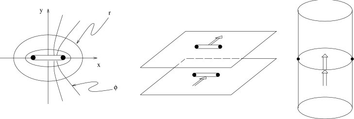
Figure 1: double cover of ${\mathbb{R}}^{2}$

The singularities are located at the branch-points $r=0,\phi=0$ and $\pi$, which is also the location where the curvature is concentrated. In order to show this let us “regularize” (1) Generalized Kerr-Schild class) by replacing $r^{2}\rightarrow r^{2}+\alpha^{2}$.

$$ds^{2} =a^{2}(\frac{f^{2}}{g^{2}}\cosh^{2}udu^{2}+f^{2}d\phi^{2})\qquad f^{2}=\sinh^{2}u+\sin^{2}\phi+\beta^{2}$$

$$r=a\sinh u,\>\alpha=a\beta g^{2}=\cosh^{2}u+\beta^{2}$$ (7)

Using an adapted frame one obtains the connection and the Riemann-tensor

$$e^{u}=a\frac{f}{g}du\qquad \omega^{u}{}_{\phi}=\frac{\cos\phi\sin\phi\cosh u}{f^{2}g}du-\frac{g\sinh u}{f^{2}}d\phi$$

$$e^{\phi}=afd\phi R^{u}{}_{\phi}=-\frac{\beta^{2}(f^{2}+2\cos\phi)\cosh u}{f^{4}g}dud\phi.$$ (8)

Evaluating the densitized Ricci tensor

$$\sqrt{g}R^{a}{}_{b}=-\frac{\beta^{2}(f^{2}+2\cos^{2}\phi)\cosh u}{f^{4}g}(\partial_{u}^{a}du_{b}+\partial_{\phi}^{a}d\phi_{b})=:F(x)(\partial_{u}^{a}du_{b}+\partial_{\phi}^{a}d\phi_{b})$$

on an arbitrary test-function $$\varphi(x)$$ gives

$$\lim\limits_{\beta\to 0}\int F(x)\varphi(x)d^{2}x=-\int\frac{\beta^{2}(f^{2}+2\cos^{2}\phi)\cosh u}{f^{4}g}\varphi(u,\phi)dud\phi$$

$$=-\left(\int\limits_{-\infty}^{\infty}du\int\limits_{-\frac{\pi}{2}}^{\frac{\pi}{2}}d\phi\>\varphi(u,\phi)+\int\limits_{-\infty}^{\infty}du\int\limits_{-\frac{\pi}{2}}^{\frac{\pi}{2}}d\phi\>\varphi(u,\phi+\pi)\right)\frac{\beta^{2}(f^{2}+2\cos^{2}\phi)\cosh u}{f^{4}g}$$

$$=-2\pi(\varphi(0,0)+\varphi(0,\pi))=-2\pi(\delta(u)\delta(\sin\phi),\varphi)$$ (9)

which explicitly shows that (1) Generalized Kerr-Schild class) when extended to the cylinder is no longer flat but develops curvature concentrated on the branch points. Since the main difference between (1) Generalized Kerr-Schild class) between and (1) Generalized Kerr-Schild class) is the breaking of the $U(1)$ symmetry down to ${\mathbb{Z}}_{2}$ it is obvious that we can no longer use the former as part of the smooth structure.

2) A short review of Colombeau theory

The expression for the Ricci tensor of the generalized Kerr-Schild class involves terms which are products of singular quantities like the curvature of the background and the profile $\hat{f}$. Within distribution theory such products are in general meaningless. There exists however a recent generalization due to Colombeau [11, 13] which embeds distribution space $\mathcal{D}^{\prime}$ into the larger algebra $\mathcal{G}$ of generalized functions. We will sketch the ideas of its construction only briefly and refer the reader to [11, 13, 14, 15] for a more detailed treatment. The main idea is to consider one-parameter families of $C^{\infty}$ functions $(f_{\epsilon})_{0<\epsilon<1}$ as basic objects. They form an algebra under the naturally defined pointwise operations. The usual $C^{\infty}$ functions are embedded as constant sequences, which does not require any additional structure. On the other hand the embedding of $C^{p}$ functions and distributions is achieved by convolution with an appropriate smoothing kernel $\rho$ via

$$f_{\epsilon}(x)=\int d^{n}y\frac{1}{\epsilon^{n}}\rho(\frac{y-x}{\epsilon})f(y).$$

Since $C^{\infty}$ functions are obviously of class $C^{p}$, consistency requires the identification of the different embeddings. The difference of the two embeddings belongs to the set of so-called negligible families, which vanish faster than any given positive power of $\epsilon$ on any given compact set. Since we want this set to be an ideal, in order to preserve the algebra structure under the identification, one has to require a growth condition in $\epsilon$ on the general families. These so-called moderate families do not grow faster than inverse powers of $\epsilon$ in the limit $\epsilon\to 0$. It can be shown that the embedding of distributions generates moderate families [11, 13].

Generalized functions (elements of $\mathcal{G}$) are thus equivalence classes of moderate families modulo negligible ones. (This situation is actually very similar to the one encountered in $L^{p}$ spaces where in our case the negligible functions play the role of measurable functions that vanish outside a set of measure zero.)

The contact with usual distribution theory is achieved by coarse-graining $\mathcal{G}$. The idea is to pack together different Colombeau-objects that give the same distribution in the limit $\epsilon\to 0$:

$$(f_{\epsilon})\in{\mathcal{G}}\approx T\in{\mathcal{D}}^{\prime}\quad\text{if}\qquad\forall\varphi\in{\mathcal{D}}\qquad\lim_{\epsilon\to 0}\int dxf_{\epsilon}(x)\varphi(x)-(T,\varphi)=0,$$

or more generally

$$(f_{\epsilon})\in{\mathcal{G}}\approx(g_{\epsilon})\in{\mathcal{G}}\quad\text{if}\qquad\forall\varphi\in{\mathcal{D}}\qquad\lim_{\epsilon\to 0}\int dx(f_{\epsilon}(x)-g_{\epsilon}(x))\varphi(x)=0.$$

The equivalence relation, which is usually called association, respects addition, multiplication by $C^{\infty}$ functions and differentiation. However it does not respect multiplication, which is to be expected since it models distributional equality within $\mathcal{G}$. Let us now come back to the question raised at the beginning of this section which is essentially boils down to the existence of a distribution that is associated with the product of $P(1/x)$ with $\delta(x)$. Within $\cal G$ we have the following representations

$$P_{\epsilon}(\frac{1}{x})=\frac{x}{x^{2}+\epsilon^{2}}\quad\text{and}\quad\delta_{\epsilon}(x)=\frac{\epsilon}{\pi}\frac{1}{x^{2}+\epsilon^{2}}.$$

In order to find the a distribution associated to their product we have to evaluate

$$\lim_{\epsilon\to 0}\int dx\frac{\epsilon x}{\pi(x^{2}+\epsilon^{2})^{2}}\varphi(x)=\int dx\frac{1}{\epsilon\pi}\frac{x}{(1+x^{2})^{2}}\varphi(\epsilon x)=\frac{1}{2}\varphi^{\prime}(0),$$

where the second equality is achieved by rescaling $x$. This shows that

$$P_{\epsilon}(\frac{1}{x})\delta_{\epsilon}(x)\approx-\frac{1}{2}\delta^{\prime}(x).$$

As we will see in the next section this is precisely what happens in the case of the extended Kerr-geometry namely the delta-function contribution from the background Ricci tensor combines with the principal value of the profile to produce derivatives of the delta-function.

3) Energy-momentum tensor of the maximally analytic Kerr geometry

As already pointed out in the introduction, the flat background in the Kerr-Schild decomposition of the Kerr-geometry becomes singular under the extension to the maximally analytic manifold. The strategy we are going to propose in this chapter is to regularize (embed into $\mathcal{G}$) the Kerr-geometry such that it stays in the generalized Kerr-Schild class.

Using the same method as in the two-dimensional example presented in section one, namely replacing $r^{2}$ by $r^{2}+\alpha^{2}$, the background-metric and the vector field become

$$ds^{2}=-dt^{2}+\frac{\Sigma+\alpha^{2}}{r^{2}+a^{2}+\alpha^{2}}dr^{2}+(\Sigma+\alpha^{2})d\theta^{2}+(r^{2}+a^{2}+\alpha^{2})\sin^{2}\theta d\phi^{2},$$

$$k^{a}=\partial_{t}^{a}+\partial_{r}^{a}-\frac{a}{r^{2}+a^{2}+\alpha^{2}}\partial_{\phi}^{a}.$$ (10)

Calculating the norm of the latter gives

$$g_{ab}k^{a}k^{b}=-1+\frac{\Sigma+\alpha^{2}}{r^{2}+a^{2}+\alpha^{2}}+\frac{a^{2}\sin^{2}\theta}{r^{2}+a^{2}+\alpha^{2}}=0,$$

which is the first condition for belonging to the generalized Kerr-Schild class. In addition we have to check the geodeticity of $k^{a}$. The simplest way to do this is to observe that $(k\nabla)k^{a}=0$ is equivalent to $k\rfloor dk=0$ due to the null character of $k^{a}$.

$$dk=-\frac{2a^{2}\cos\theta\sin\theta}{r^{2}+a^{2}+\alpha^{2}}d\theta dr-2a\cos\theta\sin\theta d\theta d\phi$$

$$k\rfloor dk=\frac{2a^{2}\cos\theta\sin\theta}{r^{2}+a^{2}+\alpha^{2}}d\theta-\frac{2a^{2}\cos\theta\sin\theta}{r^{2}+a^{2}+\alpha^{2}}d\theta=0,$$

which is the desired result, showing that the deformation still belongs to generalized Kerr-Schild class.

The first step in the evaluation of the Ricci-tensor $\tilde{R}^{a}{}_{b}$ (1) Generalized Kerr-Schild class) is the calculation of the background contribution $R^{a}{}_{b}$. Changing the radial coordinate $r$ to $r=a\sinh u$

$$g_{ab}=-dt_{a}dt_{b}+\frac{f^{2}}{g^{2}}a^{2}\cosh^{2}udu_{a}du_{b}+a^{2}f^{2}d\theta_{a}d\theta_{b}+a^{2}g^{2}\sin^{2}\theta d\phi_{a}d\phi_{b}$$

$$f^{2}=\sinh^{2}u+\cos^{2}\theta+\beta^{2}\quad g^{2}=\cosh^{2}u+\beta^{2}\qquad\alpha=a\beta$$ (11)

and using an adapted frame

$$e^{t}_{a}=dt_{a} E^{a}_{t}=\partial^{a}_{t}$$

$$e^{u}_{a}=\frac{af\cosh u}{g}du_{a} E^{a}_{u}=\frac{g}{af\cosh u}\partial_{u}^{a}$$

$$e^{\theta}_{a}=afd\theta_{a} E^{a}_{\theta}=\frac{1}{af}\partial^{a}_{\theta}$$

$$e^{\phi}_{a}=ag\sin\theta d\phi_{a} E^{a}_{\phi}=\frac{1}{ag\sin\theta}\partial^{a}_{\phi}$$ (12)

we obtain for the connection and the Riemann tensor

$$\omega^{u}{}_{\theta}=-\frac{\cos\theta\sin\theta}{f^{2}g}du-\frac{g\sinh u}{f^{2}}d\theta R^{u}{}_{\theta}=-\frac{\beta^{2}\cosh u(\sin^{2}\theta+g^{2})}{f^{4}g}dud\theta$$

$$\omega^{u}{}_{\phi}=-\frac{\sinh u\sin\theta}{f}d\phi R^{u}{}_{\phi}=-\frac{\beta^{2}\cosh u\sin\theta}{f^{3}}dud\phi$$

$$\omega^{\theta}{}_{\phi}=-\frac{g\sin\theta}{f}d\phi R^{\theta}{}_{\phi}=-\frac{\beta^{2}g\sin\theta}{f^{3}}d\theta d\phi,$$ (13)

which in turn gives rise to the mixed Ricci density

$$\sqrt{g}R^{a}{}_{b}=\frac{2a\beta^{2}\cosh u\sin\theta}{f^{4}}(g^{2}\partial^{a}_{u}du_{b}+\sin^{2}\theta\partial^{a}_{\theta}d\theta_{b}).$$

Proceeding along the lines of the example presented in the first section we obtain the associated distribution

$$\sqrt{g}R^{a}{}_{b}=2\pi a\delta(u)\delta(\cos\theta)(\partial^{a}_{u}du_{b}+\partial^{a}_{\theta}d\theta_{b}).$$

After factoring out the $k^{a}$-dependence the remaining terms become

$$\tilde{R}^{a}{}_{b}-R^{a}{}_{b} =-\frac{1}{2}k^{a}(2\hat{f}k^{c}R_{cb}-\nabla_{b}h-\hat{f}\Delta k_{b}+2\nabla_{c}\hat{f}\nabla^{c}k_{b})$$

$$+\frac{1}{2}k_{b}(\nabla^{a}h-\nabla^{2}\hat{f}k^{a}+\hat{f}\Delta k^{a}-2\nabla_{c}\hat{f}\nabla^{c}k^{a})$$

$$+(h\frac{1}{2}(\nabla_{b}k^{a}+\nabla^{a}k_{b})-\hat{f}\nabla_{c}k^{a}\nabla^{c}k_{b}))+\hat{f}R^{a}{}_{cdb}k^{c}k^{d},$$ (14)

where

$$h:=\hat{f}\nabla k+(k\nabla)\hat{f}\qquad\Delta k_{a}:=(d*d*+*d*d)k_{a}=-\nabla^{2}k_{a}+R^{b}{}_{a}k_{b}.$$

Using the Laplace-Beltrami $\Delta$ operator instead of the covariant Laplacian $\nabla^{2}$ considerably facilitates the calculation of $\nabla^{2}k^{a}$. Let us briefly state some useful identities and then present the final result.

$$\nabla_{b}k^{a}=\frac{\sinh u(g^{2}-f^{2})}{ag^{2}f^{2}}E_{u}^{a}e^{u}_{b}+\frac{\sinh u}{af^{2}}E_{\theta}^{a}e^{\theta}_{b}+\frac{\sinh u}{ag^{2}}E_{\phi}^{a}e^{\phi}_{b}$$

$$+\frac{\sin\theta\cos\theta}{agf^{2}}(E_{\theta}^{a}e^{u}_{b}-E_{u}^{a}e^{\theta}_{b})+\frac{\sinh u\sin\theta}{ag^{2}f}(E_{\phi}^{a}e^{u}_{b}+E_{u}^{a}e^{\phi}_{b})+\frac{\cos\theta}{agf}(E_{\theta}^{a}e^{\phi}_{b}-E_{\phi}^{a}e^{\theta}_{b})$$

$$\nabla^{2}\hat{f}=-\frac{8m\beta^{2}\sinh u}{a^{3}f^{8}}(g^{2}+\sin^{2}\theta)\qquad\Delta k_{a}=\frac{2}{a^{2}gf^{5}}(f^{4}-2g^{2}\beta^{2})e^{u}_{a}-\frac{2\sin\theta}{a^{2}gf^{2}}e^{\phi}_{a}$$

$$R^{a}{}_{cdb}k^{c}k^{d}=\frac{\beta^{2}}{a^{2}f^{4}}\left(\frac{\sin^{2}\theta}{g^{2}}E_{u}^{a}e^{u}_{b}+\frac{2\sin^{2}\theta+g^{2}}{g^{2}}E_{\theta}^{a}e^{\theta}_{b}+\frac{f^{2}}{g^{2}}E_{\phi}^{a}e^{\phi}_{b}+\right.$$

$$\left.\hskip 56.9055pt\frac{f\sin\theta}{g^{2}}(E_{u}^{a}e^{\phi}_{b}+E_{\phi}^{a}e^{u}_{b})\right)$$ (15)

Putting everything together gives

$$\tilde{R}^{a}{}_{b}- R^{a}{}_{b}=\frac{2\beta^{2}}{a^{2}f^{6}}\hat{f}\left[-(f^{2}+2\sin^{2}\theta)\partial_{t}^{a}dt_{b}+\frac{3f^{2}\sin^{2}\theta+2\sin^{4}\theta+f^{4}}{\sin^{2}\theta}\right.$$

$$(\frac{\sin\theta}{g}E_{\phi}^{a})(\frac{\sin\theta}{g}e^{\phi}_{b})+(f^{2}+\sin^{2}\theta)\partial_{t}^{a}(\frac{f}{g}e^{u}_{b})-2(f^{2}+\sin^{2}\theta)\partial_{t}^{a}(\frac{\sin\theta}{g}e^{\phi}_{b})$$

$$\left.+2(f^{2}+\sin^{2}\theta)(\frac{\sin\theta}{g}E_{\phi}^{a})dt_{b}-(f^{2}+\sin^{2}\theta)(\frac{\sin\theta}{g}E_{\phi}^{a})(\frac{\sin\theta}{g}e^{\phi}_{b})\right].$$ (16)

Although the last expression looks pretty complicated only a small number of terms survive the limiting process $\beta\to 0$. The final form of the Ricci-density is

$$\sqrt{\tilde{g}}\tilde{R}^{a}{}_{b} =$$

$$2\pi\delta(\cos\theta)\left(a\delta(u)(\partial^{a}_{u}du_{b}+\partial^{a}_{\theta}d\theta_{b})+m\delta^{\prime}(u)(\partial^{a}_{t}-\frac{1}{a}\partial^{a}_{\phi})(dt_{b}+ad\phi_{b})\right).$$ (17)

The typical integrals one has to deal with in the evaluation of (3) Energy-momentum tensor of the maximally analytic Kerr geometry) are

$$\lim\limits_{\beta\to 0}\int\frac{\beta^{2}\sinh u}{f^{6}}\>\bar{\varphi}(u,\theta)dud\theta=\int\limits_{-\infty}^{\infty}du\int\limits_{-\frac{\pi}{2}}^{\frac{\pi}{2}}d\lambda\frac{\beta^{2}\sinh u}{f^{6}}\>\bar{\varphi}(u,\frac{\pi}{2}-\lambda)$$

$$=\int\limits_{-\infty}^{\infty}du\int\limits_{-\infty}^{\infty}d\lambda\frac{u}{\beta(u^{2}+\lambda^{2}+1)^{3}}\bar{\varphi}(\beta u,\frac{\pi}{2}-\beta\lambda)=\frac{\pi}{4}\partial_{u}\bar{\varphi}(0,\frac{\pi}{2})$$

which implies

$$\lim\limits_{\beta\to 0}\frac{\beta^{2}\sinh u}{f^{6}}=-\frac{\pi}{4}\delta^{\prime}(u)\delta(\cos\theta)$$

Several comments are in order. First of all one might wonder why we derived the Ricci-density instead of the Ricci-tensor as in [5]. A simple answer is that the latter has no associated distribution. However, since only the determinant of the background metric enters in $\sqrt{\tilde{g}}$ our result actually does not differ in this regard from [5]. It merely is a question of whether one considers the delta-“function” to be a scalar or a density. Our result is also very similar to that obtained in [2], in that the delta-prime term of (3) Energy-momentum tensor of the maximally analytic Kerr geometry) becomes negative in the negative $r$-region. Moreover the tensor-structure of the $m$-dependent terms coincides with those in [2]. The main difference is the presence of the background-contribution, which reflects the fact that the background itself is non-flat, thereby once again emphasizing the fact that the extended Kerr-geometry belongs to the generalized Kerr-Schild class rather than the Kerr-Schild class. Due to its tensor structure the background does not contribute to the mass or angular momentum obtained by hooking the corresponding Killing vector into (3) Energy-momentum tensor of the maximally analytic Kerr geometry).

Conclusion

In this work we made use of the generalized Kerr-Schild class to calculate the energy-momentum tensor for the extension of the Kerr-geometry that contains the negative mass region. It might seem somewhat surprising to use the generalized Kerr-Schild class, since Kerr is usually considered to be a member of the (normal) Kerr-Schild class. However, a closer (distributional) look at the “flat” part of the decomposition reveals that it develops a branch-singularity upon extending to the negative $r$-sheet, and that it is therefore no longer flat. For the same reason we may no longer consider it as part of the smooth structure. Using techniques developed for the multiplication of singular expressions (Colombeau’s algebra of new generalized functions) we show that it is possible obtain a distributional energy-momentum tensor for the extended geometry, which is concentrated on the ring-singularity. Our result is consistent with [2]. The main difference arises from the presence of the background curvature terms. Due to their tensor structure the latter do not contribute to the momentum and and angular momentum densities. A natural further line of investigation would be the construction of the ultrarelativistic limits. However, since the background is no longer flat, the concept of boosts as its isometries has to be reconsidered.

Acknowledgement: The author wants to thank Werner Israel for his encouragement and numerous stimulating discussions and the Department of Physics and Astronomy at the University of Victoria for the hospitality during the final stages of this work.

References

• [1] Israel W, Phys.Β Rev.Β  D2, 641, (1970).
• [2] Israel W, Phys.Β Rev.Β  D15, 935, (1977).
• [3] Lopez, Nouvo Cimento 66B, 17, (1981).
• [4] Burinskii Ya, String-like Structures in Complex Kerr-geometry, gr-qc 9303003, and references therein.
• [5] Balasin H and Nachbagauer H, Class.Β Quantum Grav.Β  11, 1453 (1994).
• [6] Balasin H and Nachbagauer H,Class.Β Quantum Grav.Β  12, 707 (1995).
• [7] Balasin H and Nachbagauer H, Class.Β Quantum Grav.Β  13, 731 (1996).
• [8] LoustΓ³ C and SΓ‘nchez N, Nucl.Β Phys.Β B383 377 (1992).
• [9] Debney G C, Kerr R P and Schild A, J.Β Math.Β Phys.Β 10, 183 (1969).
• [10] Taub A H, Ann.Β Phys.Β 134, 326 (1981)
• [11] Colombeau J, New Generalized Functions and Multiplication of Distributions Mathematics Studies 84, North Holland (1984).
• [12] Jordan P Ehlers J and Kundt W, Akad.Β Wiss.Β Lit. (Mainz) Abhandl.Β Math.-Nat.Β Kl.Β  2, 21 (1960).
• [13] Colombeau J, Multiplication of Distributions LNM 1532, Springer (1992).
• [14] Aragona J and Biagioni H, Analysis Mathematica 17, 75 (1991).
• [15] Balasin H, Colombeau’s Generalized Functions on Arbitrary Manifolds, gr-qc/9610017, Alberta-Thy-35-96, TUW96-20