BLACK HOLE FORMATION FROM MASSIVE SCALAR FIELDS

Abstract

It is shown that there exists a range of parameters in which gravitational collapse with a spherically symmetric massive scalar field can be treated as if it were collapsing dust. This implies a criterion for the formation of black holes depending on the size and mass of the initial field configuration and the mass of the scalar field.

I INTRODUCTION

An important issue in General Relativity is to ascertain whether a given matter distribution will collapse to form a black hole. To address one aspect of this question we shall consider a minimally coupled massive scalar field with spherical symmetry which starts from rest. Massive scalar fields are important in many models of the early universe. If any of these fields underwent gravitational collapse then the result would be a primordial black hole.

In recent years, gravitational collapse with massless scalar fields and spherical symmetry has been analysed in some detail [2, 3, 4, 5]. One result to come out of this is that, when the initial profile of the scalar field is fixed in terms of a single parameter, there is a critical parameter value. Beyond the critical value a black hole will form[4].

Much less is known about the spherically symmetric collapse of massive scalar fields. In order to obtain an approximate solution of the Einstein equations we introduce a WKB approximation for the field in the limit where the mass of the scalar field is large. To leading order, the solution behaves in the same way as inhomogeneous dust. This is known already for the linearised Einstein equations, but we find that the WKB approximation is equally good in the non-linear regime.

The dust solution, like the Oppenheimer-Snyder[6] solution, always collapses to a black hole. By keeping track of the size of the terms that are higher order in the approximation we obtain a sufficient condition for the validity of the approximation and therefore for the gravitational collapse of the massive scalar field. This condition can be obtained analytically when the initial density has a top-hat form, and numerically otherwise.

Planck units (in which $G=c=\hbar=1$) are used throughout.

II THE MODEL

The most general spherically symmetric spacetime metric can be written in the form

$${\rm d}s^{2}=-{\rm e}^{2\Psi}{\rm d}\tau^{2}+{\rm e}^{-2\Lambda}{\rm dr}^{2}+R^{2}{\rm d}\Omega^{2},$$ (1)

where $\Psi=\Psi(\tau,r)$, $\Lambda=\Lambda(\tau,r)$, $R=R(\tau,r)$ and ${\rm d}\Omega^{2}={\rm d}\theta^{2}+\sin\theta{\rm d}\phi^{2}$ is the metric of a unit 2-sphere. It is convenient, for our purposes, to rescale the coordinate $\tau$ to the proper time $t$ of a comoving observer at radial coordinate $r$,

$$t=\int_{0}^{\tau}{\rm e}^{\Psi(\tau^{\prime},r)}{\rm d}\tau^{\prime},$$ (2)

hence one gets the metric in Gaussian coordinates,

$${\rm d}s^{2}=-{\rm d}t^{2}+{\rm e}^{-2\Lambda}{\rm d}r^{2}+R^{2}{\rm d}\Omega^{2}.$$ (3)

The Einstein tensor components are

$$G_{tt} = R^{-2}\left[-R{\rm e}^{2\Lambda}(2R^{\prime}\Lambda^{\prime}+2R^{\prime\prime}+R^{-1}R^{\prime 2})-2{\dot{R}}{\dot{\Lambda}}R+1+{\dot{R}}^{2}\right]$$ (4)

$$G_{rt} = -2R^{-1}({\dot{R}^{\prime}}+R^{\prime}{\dot{\Lambda}})$$ (5)

$$G_{rr} = -R^{-2}\left[{\rm e}^{-2\Lambda}(2{\ddot{R}}R+{\dot{R}}^{2}+1)-R^{\prime 2}\right]$$ (6)

$$G_{\theta\theta} = \sin^{-2}\theta G_{\phi\phi}=R[{\dot{R}}{\dot{\Lambda}}+R^{\prime}\Lambda^{\prime}e^{2\Lambda}+R^{\prime\prime}e^{2\Lambda}-{\ddot{R}}+{\ddot{\Lambda}}R-{\dot{\Lambda}}^{2}R]$$ (7)

where $\partial_{t}\equiv\;\cdot$, $\partial_{r}\equiv\;^{\prime}$.

For the matter content, we will take a real minimally coupled scalar field of mass $\mu$, whose equation of motion is

$$(-\nabla^{2}+\mu^{2})\phi=0.$$ (8)

In the spherically symmetric metric,

$$\ddot{\phi}-e^{2\Lambda}\phi^{\prime\prime}+\mu^{2}\phi+\left(\dot{\Lambda}+2R^{-1}\dot{R}\right)\dot{\phi}-e^{2\Lambda}\left(\Lambda^{\prime}-2R^{-1}R^{\prime}\right)\phi^{\prime}=0$$ (9)

The stress-energy tensor of the scalar field has components

$$T_{tt} = \frac{1}{2}{\dot{\phi}}^{2}+\frac{1}{2}{\rm e}^{2\Lambda}\phi^{\prime 2}+\frac{1}{2}\mu^{2}\phi^{2}$$ (10)

$$T_{rt} = {\dot{\phi}}\phi^{\prime}$$ (11)

$$T^{r}_{r} = \frac{1}{2}{\dot{\phi}}^{2}+\frac{1}{2}{\rm e}^{2\Lambda}\phi^{\prime 2}-\frac{1}{2}\mu^{2}\phi^{2}$$ (12)

$$T_{\theta\theta} = \sin^{-2}\theta T_{\phi\phi}=\frac{1}{/}2R^{2}({\dot{\phi}}^{2}-e^{2\Lambda}\phi^{\prime 2}-\mu^{2}\phi^{2})$$ (13)

It proves convenient to introduce the functions

$$k(t,r) = 1-{\rm e}^{2\Lambda}R^{\prime 2}$$ (14)

$$m(t,r) = \frac{1}{/}2R({\dot{R}}^{2}+k),$$ (15)

so that two Einstein equations can be recast in terms of the first derivatives of these two functions,

$${\dot{k}} = 8\pi RR^{\prime}T^{r}_{t}$$ (16)

$${\dot{m}} = 4\pi R^{2}R^{\prime}T^{r}_{t}-4\pi R^{2}{\dot{R}}T^{r}_{r}$$ (17)

These two equations, together with the scalar equation (9), form a complete set. A third Einstein equation provides a constraint

$$m^{\prime}=4\pi R^{2}R^{\prime}T_{tt}-4\pi R^{2}{\dot{R}}T_{rt}$$ (18)

which is important for relating $m(r,0)$ to the initial data.

The equations have an approximate solution when the compton wavelength of the field $\mu^{-1}$ is much smaller than the radius $\lambda$ of the spherical region where the field is non-vanishing,

$$\lambda\mu\gg 1$$ (19)

The scalar field has a wave-like solution with nearly constant amplitude,

$$\phi(t,r)=\mu^{-1}\Phi(t,r)\cos(\mu t).$$ (20)

The stress-energy tensor becomes

$$T_{tt} = \frac{1}{/}2\Phi^{2}-\frac{1}{/}2\mu^{-1}\Phi\dot{\Phi}\sin\;2\mu t+\frac{1}{/}4\mu^{-2}(\dot{\Phi}^{2}+e^{4\Lambda}\Phi^{\prime 2})(1+\cos\;2\mu t)$$ (21)

$$T_{rt} = -\frac{1}{/}2\mu^{-1}\Phi\Phi^{\prime}\sin\;2\mu t+\frac{1}{/}2\mu^{-2}\dot{\Phi}\Phi^{\prime}(1+\cos\;2\mu t)$$ (22)

$$T^{\ r}_{r} = -\frac{1}{/}2\Phi^{2}\cos\;2\mu t-\frac{1}{/}2\mu^{-1}\Phi\dot{\Phi}\sin\;2\mu t+\frac{1}{/}4\mu^{-2}(\dot{\Phi}^{2}+e^{4\Lambda}\Phi^{\prime 2})(1+\cos\;2\mu t)$$ (23)

$$T_{\theta\theta} = \frac{1}{/}2R^{2}\left[-\Phi^{2}\cos\;2\mu t-\mu^{-1}\Phi\dot{\Phi}\sin\;2\mu t+\frac{1}{/}2\mu^{-2}(\dot{\Phi}^{2}-e^{4\Lambda}\Phi^{\prime 2})(1+\cos\;2\mu t)\right]$$ (24)

The form of the stress-energy tensor suggests a trigonometric expansion for the function $\Phi$ of the form

$$\Phi=\Phi_{0}+\sum_{m=1}^{\infty}\sum_{n=2}^{2m}\,\mu^{-m}\left(\Phi^{c}_{mn}\cos\;n\mu t+\Phi^{s}_{mn}\sin\;n\mu t\right)$$ (25)

with similar expansions for $m$ and $k$. More precisely, we take

$$\Phi(t,r) = \Phi_{01}(t,r)\cos\mu t+\mu^{-2}\Phi_{22}\cos 2\mu t+O(\mu^{-3})$$ (26)

$$m(t,r) = m_{0}(t,r)+\mu^{-1}m_{12}(t,r)\sin 2\mu t+\mu^{-2}m_{22}(t,r)\cos 2\mu t+O(\mu^{-3})$$ (27)

$$k(t,r) = k_{0}(t,r)+\mu^{-2}k_{22}(t,r)\cos 2\mu t+O(\mu^{-3})$$ (28)

$$R(t,r) = R_{0}(t,r)+\mu^{-2}R_{22}(t,r)\cos 2\mu t+O(\mu^{-3})$$ (29)

Terms which play no role have been dropped.

When the expansions are substituted into eqs. (15–17) the leading order terms give

$$\dot{m}_{0} = 0$$ (30)

$$\dot{k}_{0} = 0$$ (31)

$$\dot{R}^{2}_{0} = 2m_{0}R_{0}^{-1}-k_{0}$$ (32)

$$m_{0}^{\prime} = 2\pi R_{0}^{2}R_{0}^{\prime}\Phi_{0}^{2}$$ (33)

The first three equations also arise in the Tolman–Bondi solution representing the collapse of spherically symmetric dust. We deduce that to leading order the metric will have Tolman–Bondi form.

The next order gives

$$k_{22}(t,r) = 2\pi R_{0}(R^{\prime}_{0})^{-1}(1-k_{0})\Phi_{0}\Phi^{\prime}_{0}$$ (34)

$$m_{12}(t,r) = \pi R_{0}^{2}{\dot{R}}_{0}\Phi_{0}^{2}$$ (35)

$$R_{22}(t,r) = -\frac{1}{/}2R_{0}\Phi_{0}^{2},$$ (36)

We will assume that the WKB approximation holds as long as these correction terms are less than $1/2$ the leading terms. (The effect of changing this number will be equivalent to changing the value of $\mu$). The largest correction comes from the $m_{12}$ term, therefore the WKB approximation should be valid whilst

$$\mu^{-1}{m_{12}\over m_{0}}\leq{1\over 2}$$ (37)

This inequality defines a region of the $(t,r)$ coordinate plane. The region is bounded by a curve where the inequality is saturated,

$${\dot{R}_{0}}m^{\prime}_{0}=\mu m_{0}R^{\prime}_{0}.$$ (38)

There is no reason to extend the leading order approximation beyond this curve. Therefore the region of validity of the approximation will only consist of points in whose causal past the inequality is always satisfied.

III TOLMAN–BONDI METRICS

We have seen that a sufficiently massive scalar field behaves like inhomogeneous dust. The corresponding metric can be recovered from the definitions (14) and (15), with $m(t,r)\equiv m(r)$ and $k(t,r)\equiv k(r)$ (dropping the ‘0’-indices for simplicity),

$${\rm d}s^{2} = -{\rm d}t^{2}+\frac{R^{\prime 2}(t,r)}{1-k(r)}{\rm d}r^{2}+R^{2}(t,r){\rm d}\Omega^{2}$$ (39)

$${\dot{R}}^{2}(t,r) = \frac{2m(r)}{R(t,r)}-k(r)$$ (40)

$$\Phi^{2}(t,r) = \frac{1}{2\pi}\frac{m^{\prime}}{R^{2}R^{\prime}},$$ (41)

The metric has Tolman–Bondi form [7, 8]. This is a well known class of solutions that can be thought of as a collection of free–falling spherical shells. Assuming $R^{\prime}\neq 0$ (then none of the shells cross), one can analytically integrate equation (40) parametrically

$$t(\eta,r) = t_{0}(r)+\frac{m}{k^{\frac{3}{2}}}(\eta+\sin\eta)$$ (42)

$$R(\eta,r) = \frac{2m}{k}\cos^{2}\frac{\eta}{2}$$ (43)

where $t_{0}(r)$ is an arbitrary function.

We take time-symmetric initial data with

$$R(0,r) = r$$ (44)

$${\dot{R}}(0,r) = 0$$ (45)

These initial conditions fix the radial coordinate $r$ and the functions $t_{0}(r)=0$, $k(r)=2m(r)/r$,

$$R(\eta,r) = r\cos^{2}{\eta\over 2}$$ (46)

$$t(\eta,r) = \sqrt{\frac{r^{3}}{8m}}(\eta+\sin\eta)$$ (47)

where $\eta$ runs from $0$ to $\pi$. A particular solution is uniquely specified by $m(r)$ and related to the initial density profile $T_{tt}(0,r)$,

$$m(r)=4\pi\int_{0}^{r}T_{tt}(0,r^{\prime})r^{\prime 2}dr^{\prime}$$ (48)

The function $m(r)$ is the total mass within the sphere of radius $r$. If it approaches a constant value $M$ at large radius then $M$ is the ADM mass.

A model for the initial density profile which we make use of later is

$$\rho(r)\equiv T_{tt}(0,r)=\rho_{0}e^{-(r/\lambda)^{3}},$$ (49)

so that the mass function is simply,

$$m(r)=M(1-e^{-(r/\lambda)^{3}})$$ (50)

This mass distribution collapses to form a black hole of radius $2M$. The centre collapses first, and forms a singularity after a proper-time $\pi/\sqrt{8M}$. This is shown in figure 1

Also shown in figure 1 is the event horizon, obtained by solving the equation for radial null geodesics

$${{\rm d}\eta\over{\rm d}r}=\left[\pm\left({r\over 2m}-1\right)^{-1/2}R^{\prime}-{1\over 2}\gamma(\eta+\sin\eta)\right]R^{-1}$$ (51)

where

$$\gamma(r)={3\over 2}-{rm^{\prime}\over 2m}$$ (52)

with the boundary condition $R\to 2M$ as $r\to\infty$.

Various derivatives of the radial function that are of use are

$${\dot{R}} = -\left(\frac{2m}{r}\right)^{\frac{1}{2}}\tan{\eta\over 2}$$ (53)

$$R^{\prime} = \cos^{2}{\eta\over 2}+{1\over 2}\gamma\left(\eta+\sin\eta\right)\tan{\eta\over 2}$$ (54)

The value of $\Phi$ given by eq. (41) will diverge if $R^{\prime}=0$, from which we obtain a restriction on the initial mass distribution: $\gamma\geq 0$.

IV THE OPPENHEIMER–SNYDER LIMIT

Oppenheimer and Snyder considered the collapse of a star with constant density, for which

$$m(r)=\cases{\displaystyle M\left({r\over\lambda}\right)^{3}&$0<r<\lambda$\cr M&$r\geq\lambda$}$$ (55)

In this case the model can be solved explicitly and we can obtain analytic expressions for the domain of validity of the WKB approximation. We are especially interested in those cases where the domain of validity covers the whole region outside the event horizon.

A constant scalar field gives a constant density but the discontinuity at $r=\lambda$ causes the WKB approximation to break down. It is possible to change the form of the field close to the edge to make the field continuous and still have constant density,

$$\Phi=\cases{\Phi_{0}&$r\leq\lambda-\mu^{-1}$\cr\Phi_{1}(r)&$\lambda-\mu^{-1}<r<\lambda$\cr 0&$r\geq\lambda$}$$ (56)

where $\Phi_{0}=O(1)$ and $\Phi_{1}^{\prime}=O(1)$.

The WKB approximation breaks down along the curve given by equation (38). Let $\eta_{*}(r)$ parameterise this curve, then from eqs. (53) and (54),

$$\tan{\eta_{*}\over 2}={\mu\over 3}\sqrt{\lambda^{3}\over 2M}\cos^{2}{\eta_{*}\over 2}.$$ (57)

Therefore $\eta_{*}(r)$ is constant for $r<\lambda$. In this case $t(\eta_{*},r)$ is also constant. The Tolman-Bondi solution is exact for $r>\lambda$, therefore the WKB approximation breaks down along a line segment from $r=0$ to $r=\lambda$ with fixed time coordinate $t_{*}$. If this line segment lies inside the event horizon of the Tolman–Bondi metric then the WKB approximation must be valid outside of the event horizon. This is shown in figure 2.

The event horizon is given by a curve $\eta_{EH}(r)$. Outside of the matter distribution the event horizon lies along $R=2M$, therefore

$$\cos^{2}{\eta_{EH}(r)\over 2}={2M\over r}\;\;\;r\geq\lambda$$ (58)

Now, the end of the line where the WKB approximation breaks down will lie inside the event horizon when

$$\eta_{*}>\eta_{EH}(\lambda)$$ (59)

which is when

$$\tan{\eta_{*}\over 2}>\sqrt{{\lambda\over 2M}-1}$$ (60)

Now, from equation (57) we have

$$\tan{\eta_{*}\over 2}\left(1+\tan^{2}{\eta_{*}\over 2}\right)={\mu\over 3}\sqrt{\lambda^{3}\over 2M}.$$ (61)

The condition that the WKB approximation breaks down inside the event horizon is therefore

$$\mu M>\frac{3}{2}\sqrt{1-\frac{2M}{\lambda}}.$$ (62)

If this inequality is satisfied, then the scalar field configuration with ADM mass $M$ which is initially constant for $r<\lambda$ will collapse to form a black hole. The arguments presented here say nothing about what happens when the inequality is not satisfied. The inequality approaches $\mu M>3/2$ when $\lambda$ is much larger than the initial Schwarzschild radius.

V INHOMOGENEOUS MODELS

For more complicated density distributions it becomes necessary to test the validity of the WKB approximation numerically. We will concentrate here on the exponential density distribution (49) given earlier and compare this to the results for the top-hat distribution of the Oppenheimer–Snyder limit.

The aim, as before, is to locate the parameter ranges for which a black hole forms because the WKB approximation holds good everywhere outside of the event horizon. The method we use is to find the curve on which the WKB approximation breaks down and find conditions which place this curve wholly inside the event horizon.

Differentiating eq. (38) gives an equation for $\eta_{*}(r)$,

$$\cos^{2}{\eta_{*}\over 2}\left[\gamma-\frac{1}{2}(3+\cot^{2}\frac{\eta_{*}}{2})\right]{{\rm d}\eta_{*}\over{\rm d}r}=\beta^{\prime}-{1\over 2}\gamma^{\prime}(\eta_{*}+\sin\eta_{*})$$ (63)

with $\eta_{*}(0)=\eta_{*}$, given by eq. (57) and

$$\gamma(r) = {3\over 2}-{rm^{\prime}\over 2m}$$ (64)

$$\beta(r) = \left(\frac{2m}{r}\right)^{\frac{1}{2}}\frac{m^{\prime}}{\mu m}$$ (65)

This equation can be solved numerically using a simple Runge-Kutta method. An example is shown in figure 1.

When the shape of initial field configuration is fixed, the model is parameterised by the scalar field mass $\mu$, the length scale $\lambda$ and the total mass $M$. The method used here only depends on the combinations $\lambda\mu$ and $M/\lambda$. The numerical results for two density distributions are shown in figure 3. Above the lines, the WKB approximation is valid outside of the event horizon and a black hole will form. This condition is sufficient but not necessary. The numerical results for the Openheimer–Snyder limit agree with the analytical result to six significant figures on the majority of data points.

VI CONCLUSIONS

We have analysed in some detail the regime in which a spherically symmetric massive scalar field can be treated as if it where dust. The result is a criterion for the formation of black holes depending on size and mass scales. The criterion depends to some extent on the form of the density distribution.

Outside of the WKB regime the solution of the Einstein equations is a more difficult problem. The most studied case is the massless limit, where echoing behaviour was discovered at the point which separates the cases which form black holes from those which do not. This point lies on the horizontal axis in figure 3. It is quite possible that the line which bounds black hole formation continues up from this point. It certainly must lie under the lines shown in the figure.

In some inflationary models of the early universe, the end of the inflationary phase is followed by a period dominated by the energy of a massive scalar field [9, 10, 11]. It has been mentioned before that the matter content of the universe behaves like dust during this period, leading to a situation in which density fluctuations grow and could form primordial black holes[12].

The length of time for which the massive scalar field dominates is limited by the decay of the field into radiation. The Tolman–Bondi models can be used to predict how much time is necessary for the collapse to a black hole. In an Einstein–de Sitter universe of density $\rho_{c}=3H^{2}/8\pi$, a region of dust with density $\rho=\rho_{c}(1+\zeta)$ collapses to a singularity in a time $t_{c}\approx\frac{1}{/}2\pi H^{-1}\bar{\zeta}^{-3/2}$, where $\bar{\zeta}$ is the volume average of $\zeta$. If the WKB approximation is valid then a black hole will form only if the scalar field has not decayed during the time $t_{c}$.

The results obtained here for the validity of the WKB approximation have been limited to asymptotically flat spacetimes and time symmetric initial data but they can be adapted to remove these limitations for applications to cosmology. We expect there to be little change to the results if the length scale $\lambda$ is smaller than the horizon size $1/H$.

We have a simple condition for validity of the WKB approximation in the Oppenheimer–Snyder limit, $M\mu\gg 1$. In the early universe, the mass within the scale $\lambda$ is given by $M=\frac{1}{/}2H^{2}\lambda^{3}$. The scalar field will behave like dust provided that $H^{2}\lambda^{3}\mu\gg 1$. If we take $H\lambda\sim 1$, then the condition becomes $\lambda\mu\gg 1$, which means that the WKB approximation is valid up to the formation of the event horizon if it is valid initially.

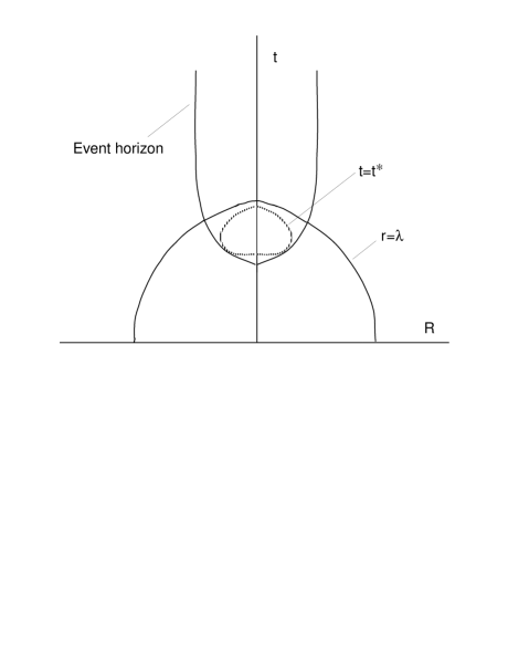
FIG. 1.: A section of the Tolman–Bondi metric with coordinates $(R,t)$ for an exponential density distribution. The shell $r=\lambda$ and the event horizon are shown, as well as the line $t=t_{*}$ where the WKB approximation breaks down..

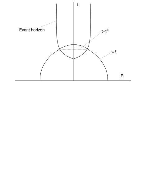
FIG. 2.: A section of the Oppenheimer-Snyder metric with coordinates $(R,t)$. The edge of the matter distribution $r=\lambda$ and the event horizon are shown, as well as the line $t=t_{*}$ where the WKB approximation breaks down.

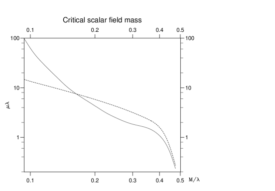
FIG. 3.: Configurations with parameters above the lines will form black holes. The dotted line denotes the top–hat field profile and the solid line denotes the exponential field profile discussed in the text. $\mu$ is the scalar field mass, $M$ the ADM mass and $\lambda$ the length scale.

REFERENCES

[1] Christodoulou, D. 1984, Commun. Math. Phys.93 171
[2]Choptuik, M. W. 1989 Frontiers in Numerical
Relativity ed C. R. Evans, L. S. Finn and D. W. Hobill (Cambridge:
Cambridge University Press).
[3]Goldwirth and Piran, T. 1987 Phys. Rev.D36
3575
[4]Choptuik, M. W 1993 Phys. Rev. Lett70 9
[5]Brady, P. R. 1994 Class. Quantum Grav.11 1255
[6] J. R. Oppenheimer and H. Sneider, Phys. Rev. 56
455 (1939)
[7] Tolman, R. C. 1934, Proc. Nat. Acad. Sci. USA20 410
[8] Bondi, H. 1948, Mon. Not. Astron. Soc.107
343
[9]Linde, A. D. 1982 Phys. Letts.B129 177.
[10]Hawking, S. W. and Moss, I. G. 1982 Phys.
Letts.B110 35
[11]Albrecht, A. and Steinhart, P. J. 1982 Phys.
Rev. Lett48 1220
[12] M. Yu. Khlopov, B. A. Malomed and Ya. B. Zel’dovich 1985
Mon. Not. R. Astron. Soc.215 517.