Searching for periodic sources with LIGO

Abstract

We investigate the computational requirements for all-sky, all-frequency searches for gravitational waves from spinning neutron stars, using archived data from interferometric gravitational wave detectors such as LIGO. These sources are expected to be weak, so the optimal strategy involves coherent accumulaton of signal-to-noise using Fourier transforms of long stretches of data (months to years). Earth-motion-induced Doppler shifts, and intrinsic pulsar spindown, will reduce the narrow-band signal-to-noise by spreading power across many frequency bins; therefore, it is necessary to correct for these effects before performing the Fourier transform. The corrections can be implemented by a parametrized model, in which one does a search over a discrete set of parameter values (points in the parameter space of corrections). We define a metric on this parameter space, which can be used to determine the optimal spacing between points in a search; the metric is used to compute the number of independent parameter-space points $N_{p}$ that must be searched, as a function of observation time $T$. This method accounts automatically for correlations between the spindown and Doppler corrections. The number $N_{p}(T)$ depends on the maximum gravitational wave frequency and the minimum spindown age $\tau=f/\dot{f}$ that the search can detect. The signal-to-noise ratio required, in order to have $99\%$ confidence of a detection, also depends on $N_{p}(T)$. We find that for an all-sky, all-frequency search lasting $T=10^{7}$ s, this detection threshhold is $h_{c}\approx(4--5)h_{\rm 3/yr}$, where $h_{\rm 3/yr}$ is the corresponding $99\%$ confidence threshhold if one knows in advance the pulsar position and spin period.

We define a coherent search, over some data stream of length $T$, to be one where we apply a correction, followed by an FFT of the data, for every independent point in the parameter space. Given realistic limits on computing power, and assuming that data analysis proceeds at the same rate as data acquisition (e.g. $10$ days of data gets analysed in $\sim 10$ days), we can place limitations on how much data can be searched coherently. In an all-sky search for pulsars having gravity-wave frequencies $f\leq 200\mbox{\rm Hz}$ and spindown ages $\tau\geq 1000\mbox{\rm Yrs}$, one can coherently search $\sim 18$ days of data on a teraflops computer. In contrast, a teraflops computer can only perform a $\sim 0.8$-day coherent search for pulsars with frequencies $f\leq 1\mbox{\rm kHz}$ and spindown ages as low as $40\mbox{\rm Yrs}$.

In addition to all-sky searches we consider coherent directed searches, where one knows in advance the source position but not the period. (Nearby supernova remnants and the galactic center are obvious places to look.) We show that for such a search, one gains a factor of $\sim 10$ in observation time over the case of an all-sky search, given a $1\mbox{\rm Tflops}$ computer.

The enormous computational burden involved in coherent searches indicates a need for alternative data analysis strategies. As an example we briefly discuss the implementation of a simple hierarchical search in the last section of the paper. Further work is required to determine the optimal approach.

I Introduction

The direct observation of gravitational waves is a realistic goal for the kilometer-scale interferometers which are now under construction at various sites around the world [1, 2]. However, the battle to see these waves is not over when the detectors are constructed and running. Searching for gravitational wave signals in the interferometer output presents its own problems, not least of which is the sheer volume of data involved.

Potential sources of gravitational waves fall roughly into three classes: bursts, stochastic background, and continuous emitters.

Burst sources produce signals which last for times considerably shorter than available observation times. The chirp signals from compact coalescing binaries belong to this class. Since theoretical waveforms, valid during the inspiral phase of the binary evolution, have been accurately calculated using post-Newtonian methods [3], it is possible to search the data stream for chirps using matched filtering techniques. Detailed studies have been carried out to ascertain the optimal set of search templates [4, 5], and a preliminary investigation of search algorithms is now under way [6]. Detection of other, not so well understood, sources in this class—e.g. non-axisymmetric supernovae—has received limited attention [7].

Flanagan [8] has determined how to cross-correllate the output of two detectors in order to search for a stochastic background of gravitational radiation, which was implemented by Compton [9] and applied to data taken during a period of 100 hours by two prototype interferometers detectors in Glasgow and Garching  [10]. In [11], Allen presents a detailed discussion of the potential significance of detecting a stochastic background. Compton’s work, and simulations performed by Allen, have demonstrated that this kind of analysis requires minimal computational resources.

In this paper we consider some issues involved in searching for continuous wave sources. Throughout our discussion we use pulsars as a guide to develop a search strategy.

A Gravitational waves from pulsars

Rapidly rotating neutron stars (pulsars) tend to be axisymmetric; however, they must break this symmetry in order to radiate gravitationally. The pulsar literature contains several mechanisms which may lead to deformations of the star, or to precession of its rotation axis, and hence to gravitational wave emission. The characteristic amplitude of gravitational waves from pulsars scales as

$$h_{c}\sim\frac{If^{2}\epsilon}{r}$$ (1)

where $I$ is the moment of inertia of the pulsar, $f$ is the gravitational wave frequency, $\epsilon$ is a measure of the deviation from axisymmetry and $r$ is the distance to the pulsar.

Pulsars are thought to form in supernova explosions. The outer layers of the star crystallize as the newborn pulsar cools by neutrino emission. Estimates, based on the expected breaking strain of the crystal lattice, suggest that anisotropic stresses, which build up as the pulsar loses rotational energy, could lead to $\epsilon\lesssim 10^{-5}$; the exact value depends on the breaking strain of the neutron star crust as well as the neutron star’s ‘geological history’, and could be several orders of magnitude smaller. Nonetheless, this upper limit makes pulsars a potentially interesting source for kilometer scale interferometers. Figure 1 shows some upper bounds on the amplitude due to these effects.

Large magnetic fields trapped inside the superfluid interior of a pulsar may also induce deformations of the star. This mechanism has been explored recently in [12], indicating that the effect is extremely small for standard neutron star models ($\epsilon\lesssim 10^{-9}$).

Another plausible mechanism for the emission of gravitational radiation in very rapidly spinning stars is the Chandrasekhar-Friedman-Schutz (CFS) instability, which is driven by gravitational radiation reaction [13, 14]. It is possible that newly-formed neutron stars may go through this instability spontaneously as they cool soon after formation. The radiation is emitted at a frequency determined by the frequency of the unstable normal mode, which may be less than the spin frequency.

Accretion is another way to excite neutron stars into emitting gravitational waves. Wagoner [15] proposed that accretion may drive the CFS instability. There is also the Zimmermann-Szedinits mechanism [16] where the principal axes of the moment of inertia are driven away from the rotational axes by accretion from a companion star. Accretion can in principle produce relatively strong radiation, since the amplitude is related to the accretion rate rather than to structural effects in the star. However, accreting neutron stars will be in binary systems, and these present problems for detection that go beyond the ones we discuss in this paper. We hope to return to the problem of looking for radiation from orbiting neutron stars in a future publication.

B Three classes of sources

Observed pulsars fall roughly into two groups: (i) young, isolated pulsars having periods of tens or hundreds of milliseconds, and (ii) older, millisecond pulsars. The young pulsars are most likely to deviate significantly from axisymmetry; however, they are generally observed to have low frequencies, so that there is a competition between the frequency, $f$, and deviation from axisymmetry, $\epsilon$, in Eq. (1). On the other hand, millisecond pulsars, whose waves are higher in frequency, tend to be quite old and well annealed into an axisymmetric configuration.

Radio observations can only probe a small portion of our galaxy in searching for pulsars. A significant effect reducing the depth of radio searches is dispersion of the signal by galactic matter between potential sources and the earth. Given current evolutionary scenarios for pulsars—that they are born in supernova explosions—it seems likely that most pulsars should be located in the galactic disk, and the youngest of these will also be shrouded in a supernova remnant, making them invisible to radio astronomers.

Blandford [17, 7] has pointed out that there could exist a class of pulsars which spin down primarily due to gravitational radiation reaction. For sources in this class the frequency scales as $f\propto\tau^{-1/4}$, where $\tau$ is the age of the pulsar. If the mean birth rate for such pulsars in our galaxy is $\tau_{B}^{-1}$, the nearest one should be a distance $r=R\sqrt{\tau_{B}/\tau}$ from earth, where $R\simeq 10$kpc is the radius of the galaxy. The intrinsic gravitational wave amplitude (that is, the amplitude $h$ at some fixed distance) of a pulsar in this class is proportional to $\tau^{-1/2}$. Thus, the nearest source in this class would have a dimensionless amplitude $h_{c}$ at the Earth

$$h\simeq 8\times 10^{-25}\left(\frac{200\mbox{\rm Yrs}}{\tau_{B}}\right)^{1/2}$$ (2)

independent of the frequency, or the the ellipticity $\epsilon$ of the pulsar. Assuming the existence of such a class of pulsars, with $\tau_{B}\lesssim 2\times 10^{4}$ Yrs, we see from Fig. 1 that there is a large region of parameter space that is both (i) detectable by the LIGO detector and (ii) physically reasonable, in the sense that $\epsilon<10^{-5}$ and $f$ lies in the range 200–1000 Hz.

Note that Blandford’s argument can be slightly re-cast to yield an upper limit on the gravitational wave strength of any isolated pulsar–i.e., any pulsar whose radiated angular momentum is not being replenished by accretion. The age of an isolated pulsar must be shorter than the age computed assuming the spin-down is solely due to gravitational wave emission. Correspondingly, if we set $\tau_{B}$ equal to $40$ yrs (corresponding to the birthrate for $\it all$ pulsars), we get the following upper limit for measured gravitational wave amplitude of an isolated pulsar: $h_{c}<2\times 10^{-24}$. Of course, this is a statistical argument. This bound could certainly be violated by an isolated pulsar that just happens to be anomalously close to us.

It is important that any search strategy should be general enough to encompass all three of the above classes, allowing for the significant changes in frequency which may be inherent in the sources (see section II).

FIG. 1.: Characteristic amplitudes $h_{c}$ [see Eq. (11)] for several postulated periodic sources, compared with sensitivities $h_{\rm 3/yr}$ of the initial and advanced detectors in LIGO. ($h_{\rm 3/yr}$ corresponds to the amplitude $h_{c}$ of the weakest source detectable with 99% confidence in $\frac{1}{3}{\rm yr}=10^{7}\mbox{\rm s}$ integration time, if the frequency and phase of the signal is known in advance.) Long-dashed lines show the expected signal strength as a function of frequency for pulsars at a distance of 10 kpc, assuming non-axisymmetries of $\epsilon=10^{-5}$ and $\epsilon=10^{-8}$, where $\epsilon$ is defined in section IIIA. Upper limits are also plotted for the Crab and Vela pulsars, assuming their entire measured spindown is due to gravitational wave emission. The dotted lines indicate the strongest waves received at the earth for Blandfords hypothetical class of pulsars; each line corresponds to a particular birth rate.

C The data analysis problem

The detection of continuous, nearly fixed frequency waves will be achieved by constructing power spectrum estimators and searching for statistically significant peaks at fixed frequencies. In practice, this is achieved by calculating the amplitude of the Fourier transform of the detector output given by applying a fast Fourier transform (FFT), a discrete approximation to the true Fourier transform:

$$\tilde{h}(f)=\frac{1}{\sqrt{T}}\int_{0}^{T}e^{2\pi ift}\;h(t)\;dt\;.$$ (3)

The main hope of detection lies in the fact that one may observe the sky for long time periods of time $T$. When such a data stretch is transformed to make the underlying signal monochromatic, the signal to noise ratio grows as $\sqrt{T}$ in amplitude (or as $T$ in the power spectrum). One will likely need to have integration times of several weeks or months in order for the expected signals from nearby sources to rise above the noise. However, such long data stretches pose a significant computational burden; using $10^{7}\mbox{\rm s}$ of data to look for signals with gravitational wave frequencies up to $500\mbox{\rm Hz}$ requires calculating an FFT with $N\simeq 10^{10}$ data points. Calculation of a single such FFT would take about $1\mbox{\rm s}$ on a $1$Tflops computer, assuming that all $10^{10}$ points can be held in fast memory. Unfortunately, this is not the whole story.

The detection problem is complicated by the fact that the signal received at the detector is not perfectly monochromatic. Earth-bound detectors participate in complex motions which lead to significant Doppler shifts in frequency as the Earth rotates, and as it orbits around the sun (this orbit is significantly perturbed by the moon and the other planets). The time dependent accelerations broaden the spectral lines of fixed frequency sources spreading power into many Fourier bins about the observed frequency. In order to maintain the benefit of long observation times, it is therefore necessary to remove the effects of the detector motion from the data stream. This can achieved by introducing an inertial (barycentered) time coordinate and carrying out the FFT with respect to it. The difficulty of doing this was first estimated by one of us [18]. However, we must also consider the additional complication that the signal may not be intrinsically monochromatic. If the signal exhibits intrinsic frequency drift, or modulation, due to the nature and location of the source — as is expected for pulsars which spin down with time — these effects can also be removed in the transformation to the new time coordinate.

Unfortunately, the demodulated time coordinate depends strongly on the direction from which the signal is expected, and on the intrinsic frequency evolution one assumes for the source. Thus, in searching for sources whose position and timing are not well known in advance one must apply many different corrections to the data, performing a new FFT after each correction. Given the possibility that the strongest sources of continuous gravitational waves may be electromagnetically invisible or previously undiscovered, an all sky, all frequency search for such unknown sources is of considerable interest. To obtain some idea of the magnitude of this task, consider searching the entire sky for signals with (fixed) frequencies up to $500\mbox{\rm Hz}$ using $10^{7}\mbox{\rm s}$ worth of data. Assuming the entire data stream could be held in fast memory on a machine capable of $1\mbox{\rm Tflops}$, it would take $10^{8}\mbox{\rm s}$ to complete the search. Introducing intrinsic spindown effects into the search increases the computational cost, at fixed integration time, by many orders of magnitude. This computational cost is the central problem of searching for unknown pulsars in the output from gravitational wave detectors and is the focus of this paper.

D Summary of results

We parametrise the space of pulsar signals by the position of the source on the sky $\{\theta,\phi\}$, entering through Doppler shifts due to the detector’s motion, and by spindown parameters $f_{k}$ which characterise the intrinsic frequency evolution. [See Eq. (13).] We constrain the range of possible values of the spindown parameters using the (spindown) age $\tau=f/\dot{f}$ of the youngest search that a search can detect, thus $|f_{k}|\leq\tau^{-k}$. For the computationally-intensive search over all sky positions and spindown parameters, it is important to be able to calculate the smallest number of independent parameter values which must be sampled in order to cover the entire space of signals. We have accomplished this by introducing a distance measure and corresponding metric on the parameter space. The analysis is patterned after a similar one developed by Owen [5] for gravitational waves from inspiralling, compact binaries. Using our metric one can compute the volume of parameter space, thus inferring the number of independent points that must be sampled in order to cover the entire space. We define a coherent search to be one where we perform one demodulation and FFT of the data for every independent point in the parameter space. Besides telling us the computational requirements for a coherent search, the metric approach tells us how to place the points most efficiently in parameter space, in a similar way to that discussed by Owen.

We have found it useful to present the results based on several possible search strategies, which cover different regions of the parameter space. Accordingly, we define a pulsar to be old if its spindown age $\tau$ is greater than $10^{3}$ Yrs and young if $\tau\gtrsim 40$ Yrs. A pulsar is considered to be slow if its gravitational wave frequency is $f\lesssim 200$ Hz and fast if $f\lesssim 10^{3}$ Hz.

A coherent all-sky search of $10^{7}$ seconds of data for old, slow pulsars requires approximately $1.1\times 10^{10}$ independent points in the parameter space; only one spindown parameter is needed to account for intrinsic frequency evolution. In contrast, an all-sky search for fast, young pulsars in $10^{7}$ seconds of data requires $8\times 10^{21}$ independent parameter space points to be sampled, using three spindown parameters to model intrinsic frequency evolution. Note that searches for old, fast pulsars (such as known millisecond radio pulsars) and young, slow pulsars (younger brothers of the Crab and Vela) are automatically subsumed under the latter search. These results mean the following. Assuming unlimited computer power and stationary, gaussian statistics, a pulsar with unknown position and period must have strain $h_{c}\approx 4.3h_{\rm 3/yr}$, if it is in our ‘old, slow’ category, and $h_{c}\approx 5.1h_{\rm 3/yr}$, if it is in our ‘young, fast’ category, to be detected with $99\%$ confidence in a $10^{7}$ second search. Here $h_{\rm 3/yr}$ is the strain required for detection with $99\%$-confidence in a $10^{7}$ second integration, assuming the pulsar position and period are known in advance:

$$h_{\rm 3/yr}(f)=4.2\,\sqrt{S_{n}(f)\times 10^{-7}Hz}\;.$$ (4)

Thus, when considering an all-sky, all-frequency pulsar search, the LIGO sensitivity curves shown in Fig.1 effectively overestimate the detector’s sensitivity by a factor of $\sim 4--5$, even in the limit of infinite computing power.

Our ability to perform searches for continuous waves will certainly be limited by the available computing resources. Assuming realistic computer power — say of order $10^{13}$ flops — we estimate that computing limitations will effectively reduce the sensitivity of the detector by another factor of $\sim 2$, even for some reasonably optimized and efficient search strategy. However more work will be needed to develop a reasonably optimized algorithm, and thus to refine this latter estimate.

While the concept of the metric is introduced in the framework of an all-sky search for unknown pulsars, it is clear that we may use the same approach to examine the depth of a search over limited regions of the parameter space. In particular, once the scope of a search is decided, the optimization procedure dicussed in section VI can be used to determine the observation time and grid spacing which maximises the expected sensitivity of a search. As an example, we consider coherent directed searches, in which one assumes a specific sky position (such as a particular cluster or supernova remnant) and searches only over spindown parameters. Again, we present results for two concrete scenarios based on fast, young pulsars and old, slow pulsars. Similar considerations apply to directed searches as to all-sky searches; that is, the curves in Fig. 1 overestimate the detector sensitivity for $10^{7}$ second integration. Table 1 summarises the results for both cases.

We note that in each type of search, the number of parameter space points, and hence the computational requirements, were reduced significantly by the assumption that the points were placed with optimal spacings given by the metric formalism. Nevertheless, the bottom line is that limitations on computational resources will severely restrict the integration times that can be achieved. Assuming access to a Tflops of computing power (effective computational throughput, ignoring possible overheads due to interprocessor communication or data access), we find the following limits on coherent integration times: For young, fast pulsars we are limited to about 0.8 days for an all-sky search, and 18 days for a directed search. For older, slower pulsars, on the other hand, we are only limited to 9 days for an all-sky search, and nearly 160 days for a directed search. The threshold sensitivities that these strategies can achieve, relative to the noise curves in Fig. 1, are plotted as functions of computing power in Fig. 2.

TABLE I.: The number of independent parameter points $N_{p}(T,\mu_{\rm max}=0.3)$ required for a coherent $T=10^{7}{\rm s}$ search, for four fiducial types of pulsar. We list the requirements both for all-sky searches and for directed searches (i.e., searches where the source position is known in advance). Also listed are the threshhold values $h_{\rm th}$ of the characteristic strain $h_{c}$ required to have $99\%$ confidence of detection, assuming unlimited computer power. These threshold values are given by $h_{\rm th}/h_{\rm 3/yr}=(1/1.90)\sqrt{\ln(50NN_{p})-1}$ where $N\equiv 2f_{\rm max}T$. Here $h_{\rm 3/yr}$ is the corresponding threshhold, assuming the pulsar’s postion and period and are known in advance.

Search Parameters		$N_{p}$	$h_{\rm th}/h_{\rm 3/yr}$	$N_{p}$	$h_{\rm th}/h_{\rm 3/yr}$
f (Hz)	$\tau$ (Yrs)	(all-sky)	(all-sky)	(directed)	(directed)
$<200$	$>10^{3}$	$1.1\times 10^{10}$	$3.7$	$3.7\times 10^{6}$	$3.3$
$<10^{3}$	$>10^{3}$	$1.3\times 10^{16}$	$4.2$	$1.2\times 10^{8}$	$3.5$
$<200$	$>40$	$1.7\times 10^{18}$	$4.3$	$8.5\times 10^{12}$	$3.9$
$<10^{3}$	$>40$	$8\times 10^{21}$	$4.6$	$1.4\times 10^{15}$	$4.1$

FIG. 2.: Relative amplitude sensitivities $h_{\rm 3/yr}/h_{\rm 1/T}$ achievable with given computational resources, for various coherent search strategies: (a) directed search for old ($\tau\geq 1000\mbox{\rm Yrs}$), slow ($f\leq 200\mbox{\rm Hz}$) pulsars, (b) all-sky search for old, slow pulsars, (c) directed search for young ($\tau\geq 40\mbox{\rm Yrs}$) fast ($f\leq 1000\mbox{\rm Hz}$) pulsars, and, (d) all-sky search for these same sources. $h_{\rm 1/T}$ is the expected sensitivity of the detector for an observation time $T$ seconds, and with $99\%$ confidence, assuming only that the frequency bandwidth of the source is constrained in advance. For a given computational power, we have determined the optimum observation time as described in sections VIB and VII.

E Organization of this paper

In section II we outline the physics of pulsars which is relevant to the detection of continuous gravitational waves. The discussion is phenomenological and based almost entirely on pulsar data collected by radio astronomers. We focus attention on effects which may lead to significant frequency evolution over periods of several weeks of observation.

Then, in section III, we introduce a parameterised model of the expected gravitational waveform, including modulating effects due to detector motion.

From this, we go on in section IV to describe the basic technique used to search for signals, by constructing a demodulated time series. Livas [19], Jones [20] and Niebauer [21] have implemented variants of this basic search strategy over limited regions of parameter space (in particular they have not considered pulsar spin-down, and have restricted attention to small areas of the sky).

For the more computationally-intensive search over all sky positions and spindown parameters, it is important to be able to calculate the smallest number of independent parameter values which must be sampled in order to cover the entire space of signals. In section V we develop the metric formalism for calculating the number of independent points in parameter space.

In sections VI and VII we apply this formalism to determine the computational requirements of an all-sky search for unknown pulsars and a directed search, respectively.

Finally in section VIII, we list some possible alternatives to a straightforward coherent search of the interferometer data. Detailed studies of the pros and cons of each are currently under investigation.

II Pulsar phenomenology

Currently, the only expected sources of continuous, periodic gravitational waves in the LIGO band are pulsars. In this section, therefore, we review those properties of pulsars which may be important in the detection process. In general, the search technique we present later is capable of detecting any nearly monochromatic gravitational wave with sufficient amplitude. However, it is useful to have a concrete physical system in mind when considering the expected gravitational waveform.

That pulsars are rapidly rotating neutron stars is now well established [22]. Their high densities and strong gravitational fields allow them to withstand rotation rates of hundreds of times per second. Moreover, pulsar emission mechanisms require large magnetic fields, frozen into (co-rotating with) the neutron star. Indeed these large field strengths may produce non-axisymmetric deformations of the pulsar. However, the most remarkable feature of pulsars is the very precise periodicity of observed pulses.

There are more than 700 known pulsars, all at galactic distances, concentrated in the galactic plane. Based on the sensitivity limits of radio observations the total number of active pulsars in our galaxy is estimated to be more than $10^{5}$ [23, 24].

A Spindown

Pulsars lose rotational energy by electromagnetic braking, the emission of particles and, of course, emission of gravitational waves [25, 26]. Thus, the rotational frequency is not completely stable, but varies over a timescale $\tau$ which is of order the age of the pulsar. Typically, younger pulsars (with periods of tens of milliseconds) have the largest spindown rates. Figure 3 shows the distribution of rotational frequencies and spindown age, $\tau=f/(df/dt)$.

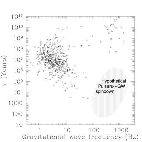
FIG. 3.: Gravitational wave frequency versus spindown age, $\tau=f/(df/dt)$, measured in years, for 540 pulsars which have measured period derivative. The figure clearly shows a large concentration of pulsars in the mid-left of diagram. Most of these are isolated pulsars. The standard evolutionary scenario suggests that pulsars move from higher frequencies and shorter spindowns left and up towards this main bunch. In contrast, many of the millisecond pulsars lying in the upper right of the figure are in binary systems, and it is widely believed that these are pulsars which have been spun up by mass accretion from the companion star.

Current observations suggest that spindown is primarily due to electromagnetic braking; however, for detection purposes it is necessary to construct a sufficiently general model of the frequency evolution to cover all possibilities. For observing times $t_{\rm obs}$, say, much less than $\tau$, the frequency drift is small and the rotational frequency can be modeled as a power series of the form

$$f(t)=(f_{0}/2)\bigl{(}1+\sum_{k}f_{k}t^{k}\bigr{)}\;.$$ (5)

If $\tau_{\rm min}$ is the shortest timescale over which the frequency is expected to change by a factor of order unity, the coefficients satisfy

$$|f_{k}|\lesssim\tau_{\rm min}^{-k}\;.$$ (6)

Clearly, for an observation time $t_{\rm obs}\ll\tau_{\rm min}$, the first few terms in this series will dominate.

Observations suggest that pulsars are born in supernova explosions with very short periods (perhaps several milliseconds), and subsequently spin down on timescales comparable to their age. Supernovae are observed in galaxies similar to our own at the rate of two or three per century, so we might expect $\tau_{\rm min}\sim 40$ years for pulsars in our galaxy. It is at this point that the distinction between various classes of pulsars becomes important. The known millisecond pulsars are old neutron stars which have have been spun up to periods of only a few milliseconds, possibly by episodes of mass transfer from a companion star. As seen from Fig. 3, timing measurements of millisecond pulsars yield very long spindown timescales, $\tau_{\rm min}\gtrsim 10^{7}$ years.

B Proper Motions

Pulsars are generally high velocity objects [25], as can be inferred by the distance they move in their lifetimes. Proper motions cause Doppler shifts in the observed pulsar frequency. If the motion is uniform (constant velocity), it simply induces a constant frequency shift — an effect which is undetectable. However, acceleration and higher order derivatives of the source’s motion will modulate the observed frequency.

Studies of millisecond pulsars in globular clusters have shown that acceleration in the cluster field can produce frequency drifts which are comparable in magnitude to the spindown effects [27, 28]. Once again, we expect these effects to be well modelled by a power series in $t/\tau_{\rm cross}$, where $\tau_{\rm cross}$ is the time it takes the pulsar to cross the cluster. We expect that $\tau_{\rm min}\leq\tau_{\rm cross}$ for these objects (since if not, the pulsar will already have escaped the cluster). Thus the frequecy model adopted above should be sufficiently general to encompass the observational effects of proper motions of the sources.

A large proportion of millisecond pulsars are also in binary systems. Unfortunately, such pulsars participate in proper motions which vary over very short timescales (their orbital periods). The time-dependent Doppler effect due to these motions is not modelled accurately by a simple power series as in Eq. (5). They would require a more elaborate model involving as many as five unknown orbital parameters. Including these effects in a coherent, all-sky search strategy would be prohibitive (see section VI). In a search for gravitational waves from a known binary pulsar, however, it would be important to deal with this effect.

Proper motions can also affect a search if the star moves across more than one resolution element on the sky during an observation. For the lengths of observation periods envisioned here, this is unlikely to be a problem. In an observation lasting a year, however, a pulsar with a spatial velocity of $1\times 10^{3}\;\rm km\;s^{-1}$ at a distance of $300\;pc$ will move by about half an arcsecond, which is comparable to the resolution limit for our observations if the pulsar frequency is 1kHz.

C Glitches

In addition to gradual frequency drifts due to spindown, some young pulsars exhibit occasional, abrupt increases in frequency. The physical mechanism behind these frequency glitches is not well understood, although the number of observations of glitch events is growing [23]. Given the stochastic nature of glitching, and the expectation that several months will elapse between major events, we will ignore glitching in this paper.

III Gravitational waves from pulsars

In order to gain insight into the detection problem it is also important to understand the expected gravitational wave signal. Several mechanisms have been discussed in the literature which may produce non-axisymmetric deformations of a pulsar, and hence lead to gravitational wave generation [12, 13, 14, 16, 29, 30].

In general, a pulsar can radiate strongly at frequencies other than twice the rotation frequency. For example, a pulsar deformed by internal magnetic stresses, which are not aligned with a principal axis, can radiate at the rotation frequency and twice that frequency [31]. If the star precesses, it will radiate at three frequencies: the rotation frequency, and the rotation frequency plus and minus the precession frequency [16]. The important point, however, is that the signal at the detector is generally narrow band, exhibiting only slow frequency drift on observational timescales.

Therefore, in this section we outline the main features of the expected waveform and the corresponding strain measured at a detector for the case of crustal deformation; other scenarios give similar results except for the presence of more than one spectral component.

A Waveform

Adopting a simple model of a distorted pulsar as a tri-axial ellipsoid, rotating about a principal axis with a frequency given by Eq. (5), one may compute the expected gravitational wave signal using the quadrupole formula. The two polarizations are

$$h_{+} = h_{0}(1+\cos^{2}i)\;\cos\{2\pi\,f_{0}\,[t+{\textstyle\sum}f_{k}{\textstyle\frac{t^{k+1}}{k+1}}]\}\;,$$ (7)

$$h_{\times} = 2h_{0}\cos i\;\sin\{2\pi\,f_{0}\,[t+{\textstyle\sum}{f_{k}}{\textstyle\frac{t^{k+1}}{k+1}}]\}\;,$$ (8)

where $i$ is the angle between the rotation axis and the line of sight to the source. The dimensionless amplitude is

$$h_{0}=\frac{8\pi^{2}G}{c^{4}}\;\frac{I_{zz}f_{0}^{2}}{r}\;\epsilon\;,$$ (9)

where

$$\epsilon=\frac{I_{xx}-I_{yy}}{I_{zz}}$$ (10)

is the gravitational ellipticity of the pulsar. The distance to the source is $r$, and $I_{jk}$ is its moment of inertia tensor.

The strength of potential sources is best discussed in terms of the characteristic amplitude $h_{c}$, defined in Eq. (50) of [7], and simply related to $h_{0}$ by

$$h_{c}=\sqrt{\frac{2}{15}}h_{0}\;.$$ (11)

For a typical $1.4M_{\odot}$ neutron star, having a radius of $10$km and at a distance of $10$kpc, the dimensionless amplitude is

$$h_{c}=7.7\times 10^{-25}\;\frac{\epsilon}{10^{-5}}\;\frac{I_{zz}}{10^{45}\mbox{ g cm}^{2}}\frac{10\mbox{kpc}}{r}\left(\frac{f_{0}}{1\mbox{kHz}}\right)^{2}\;.$$ (12)

The magnitude of the gravitational ellipticity, $\epsilon$, represents the central uncertainty in any estimate of gravitaional waves from pulsars. The tightest theoretical constraint, $\epsilon<10^{-5}$, is set by the maximum strain that the neutron star crust may support [7]. It has also been suggested that stresses induced by large magnetic fields might result in significant gravitational ellipticity. Recently, Bonazzola and Gourgoulhon [12] have considered this possibility, finding discouraging results; their calculations indicate $10^{-13}\lesssim\epsilon\lesssim 10^{-9}$ depending on the precise model they consider.

In any case, an upper bound on the gravitational ellipticity is $\epsilon\sim 10^{-5}$, although typical values may be significantly smaller.

B Signal at the detector

Observing the gravitational waves using an earth-based interferometer introduces two further difficulties into the detection process: Doppler modulation of the observed gravitational wave frequency, and amplitude modulation due to the changing orientation of the detector.

For the purpose of detection, the Doppler modulation of the observed gravitational wave frequency, due to motion of the detector with respect to the solar system barycenter, is a large effect. Assuming the intrinsic frequency model (5) for the pulsar rotation, the gravitational wave frequency measured at the detector is

$$f_{\rm gw}(t)=f_{0}\,\bigl{(}1+\sum_{k}f_{k}t^{k}\bigr{)}\bigl{(}1+\frac{\vec{v}}{c}\cdot\hat{n}\bigr{)}$$ (13)

where $\vec{v}(t)$ is the detector velocity and $\hat{n}$ is the unit vector pointing to the pulsar, in some inertial frame. We generally choose this frame to be initially comoving with the Earth at $t=0$. The frequency measured in this frame is identical to that measured at the solar system barycenter except for an unimportant constant shift in $f_{0}$.

To understand the amplitude modulation we must introduce the Euler angles, $\{\Theta,\Phi,\Psi\}$, which specify the orientation of the gravitational wave frame with respect to the detector frame. The dimensionless strain at the detector is

$$h=F_{+}(\Theta,\Phi,\Psi)h_{+}+F_{\times}(\Theta,\Phi,\Psi)h_{\times}$$ (14)

where $F_{+}$ and $F_{\times}$ are the detector beam patterns given in Thorne [7]. In searching for continuous gravitational waves from a particular direction, the Euler angles become periodic function of sidereal time, thus resulting in an amplitude and phase modulation of the observed signal [7, 12, 19]. For observation times longer than one sidereal day, the amplitude modulation effectively averages the reception over all values of right ascension, and over a range of declination which depends one the precise position of the pulsar. In particular, the effect of this process is to allow detection of continuous waves from any direction, but at the cost of reducing the measured strain (see Fig. 4).

C Parameter space

To facilitate later discussion it is useful to parameterize the gravitational waveform by a vector ${\mathchoice{{\hbox{\boldmath$\displaystyle\lambda$}}}{{\hbox{\boldmath$\textstyle\lambda$}}}{{\hbox{\boldmath$\scriptstyle\lambda$}}}{{\hbox{\boldmath$\scriptscriptstyle\lambda$}}}}=(\lambda^{0},\vec{\lambda})$ such that

$$(\lambda^{0},\lambda^{1},\ldots\lambda^{s+2})=(f_{0},n_{x},n_{y},f_{1},\ldots,f_{s})\;.$$ (15)

Here $s$ is the maximum number of spindown parameters included in the frequency model determined by Eq. (5). These vectors span an $s+3$ dimensional space on which $\lambda^{\alpha}$ can be thought of as coordinates. (Note that $n_{z}^{2}=1-n_{x}^{2}-n_{y}^{2}$ is not an independent parameter.) In particular we denote the observed phase of the gravitational waveform by

$$\phi(t;{\mathchoice{{\hbox{\boldmath$\displaystyle\lambda$}}}{{\hbox{\boldmath$\textstyle\lambda$}}}{{\hbox{\boldmath$\scriptstyle\lambda$}}}{{\hbox{\boldmath$\scriptscriptstyle\lambda$}}}})=2\pi\int^{t}\!\!dt^{\prime}\;f_{\rm gw}(t^{\prime})\;,$$ (16)

where $f_{\rm gw}(t^{\prime})$ is given by Eq. (13).

Initial interferometers in LIGO should have reasonable sensitivity to gravitational waves with frequencies

$$f\geq 40\mbox{\rm Hz}\;,$$ (17)

while advanced interferometers are expected to have improved sensitiviy down to

$$f\geq 10\mbox{\rm Hz}\;.$$ (18)

Moreover, theoretical constraints suggest that pulsars with spin periods significantly smaller than one millisecond are unlikely. This helps to constrain the highest frequency that one may wish to consider in an all sky search to be about $2\mbox{\rm kHz}$. According to the discussion in section II, the spindown parameters satisfy

$$-\tau_{\rm min}^{-k}\leq f_{k}\leq\tau_{\rm min}^{-k}\;,$$ (19)

where $\tau_{\rm min}$ is the minimum spindown age of a pulsar to be searched for. Finally, $n_{x}$ and $n_{y}$ are restricted by the relation

$$n_{x}^{2}+n_{y}^{2}\leq 1\;.$$ (20)

IV Data analysis technique

Radio astronomers are familiar with searching for nearly periodic sources in the output of their detectors [28, 32]. The technique employed by them is directly applicable to the problem at hand [19, 20].

In the detector frame the gravitational wave signal can be written as

$$h(t;{\mathchoice{{\hbox{\boldmath$\displaystyle\lambda$}}}{{\hbox{\boldmath$\textstyle\lambda$}}}{{\hbox{\boldmath$\scriptstyle\lambda$}}}{{\hbox{\boldmath$\scriptscriptstyle\lambda$}}}})={\mbox{\rm Re}}\left[{\cal A}e^{-i\phi(t;{\mathchoice{{\hbox{\boldmath$\displaystyle\lambda$}}}{{\hbox{\boldmath$\textstyle\lambda$}}}{{\hbox{\boldmath$\scriptstyle\lambda$}}}{{\hbox{\boldmath$\scriptscriptstyle\lambda$}}}})}\right]$$ (21)

where ${\cal A}=(h_{0+}+ih_{0\times})$, $h_{0+}=F_{+}(1+\cos^{2}i)h_{0}$ and $h_{0\times}=2F_{\times}(\cos i)\,h_{0}$. The orbital phase $\phi(t;{\mathchoice{{\hbox{\boldmath$\displaystyle\lambda$}}}{{\hbox{\boldmath$\textstyle\lambda$}}}{{\hbox{\boldmath$\scriptstyle\lambda$}}}{{\hbox{\boldmath$\scriptscriptstyle\lambda$}}}})$ is given by Eqs. (16) and (13). Introducing a canonical time

$$t_{b}[t;\vec{\lambda}]=\frac{\phi(t;{\mathchoice{{\hbox{\boldmath$\displaystyle\lambda$}}}{{\hbox{\boldmath$\textstyle\lambda$}}}{{\hbox{\boldmath$\scriptstyle\lambda$}}}{{\hbox{\boldmath$\scriptscriptstyle\lambda$}}}})}{2\pi f_{0}}\;,$$ (22)

the above signal becomes monochromatic as a function of $t_{b}$. (The presence of the amplitude modulation complicates the following analysis without changing the conclusions significantly; therefore, we treat $\cal A$ as constant in this and the next section.) Figure 4 shows the normalised power spectrum computed from the signal as a function of $t$ in Eq. (21) (with $f_{k}\equiv 0$), compared with the spectrum from the signal as a function of $t_{b}$. It is clear that the maximum power per frequency bin is significantly reduced when frequency modulation is not accounted for.

FIG. 4.: Power spectra for two signals, each with gravitational wave frequency $5\mbox{\rm Hz}$, computed using approximately $10$ days worth of data; they are normalised with respect to the maximum power achieved if the source was directly above an interferometer which remained stationary during the entire observation. The signal was assumed to come from declination $0^{\circ}$ and right ascension $90^{\circ}$; in fact the amplitude modulation is only sensitive to changes in declination. The detector latitude was chosen to coincide with LIGO detector in Hanford Washington. The solid line corresponds to a Doppler and amplitude modulated gravitational wave signal. The dashed line is the same signal but with the Doppler modulation removed by stretching. The (unreasonably) low frequency was chosen for illustrative purposes, so that both curves could appear on the same scale. For realistic gravitational wave frequencies ($\sim 500\mbox{\rm Hz}$) the Doppler modulated signal would be further reduced by roughly two orders of magnitude.

Radio astronomers refer to this technique of introducing a canonical time coordinate as stretching the data. Since interferometer output will be sampled at approximately $16\mbox{\rm kHz}$, in a practical search for pulsars up to $2\mbox{\rm kHz}$ gravitational wave frequency, the stretching can probably be achieved by resampling the data stream appropriately. This method, which is called stroboscopic sampling by Schutz [18], has the benefit of keeping the computational overhead introduced by the stretching process to a minimum. We will return to this issue in a later publication.

Now, a search of the detector output, $o(t)$, for gravitational waves from a known source is straightforward. One assumes specific parameter values $\vec{\xi}$ in the waveform (21), computes the demodulated time function $t_{b}[t;\vec{\xi}\,]$ using Eq. (22) and stretches the detector output accordingly, thus

$$o_{b}(t_{b}[t;\vec{\xi}\,])=o(t)\;.$$ (23)

If the assumed parameters $\vec{\xi}$ are not too much different from the actual parameters $\vec{\lambda}$ of the signal, the stretched data will consist of a nearly monochromatic signal. One then takes the Fourier transform with respect to $t_{b}$,

$$\tilde{o}(f;\vec{\xi}\,)=\frac{1}{\sqrt{T_{b}^{\mbox{\rm obs}}}}\int_{0}^{T_{b}^{\mbox{\rm obs}}}e^{2\pi ift_{b}}\;o_{b}(t_{b})\;dt_{b}\;.$$ (24)

Here $T_{b}^{\mbox{\rm obs}}$ is length of the observation measured using $t_{b}$. The power spectrum is then searched for excess power. (The threshold is set by demanding some overall statistical significance for a detection; see section VI.) Notice that the gravitational wave frequency, $\lambda^{0}=f_{0}$, is treated somewhat differently than the other parameters; the Fourier transform searches over all possible values in a single pass. Given a sampled data set containing $N$ points, the entire process, from original data through to the power spectrum, requires of order $3N\log_{2}N$ floating point operations (to first approximation).

If all the parameters are not known accurately in advance, it will be necessary to search over some of the remaining parameters $\vec{\lambda}$; a separate demodulation and FFT must be performed for each independent point in parameter space that one wishes to search. There are many possible refinements on this strategy which could reduce the computational cost of a search by circumventing certain stages of the procedure described here. We mention some of them in section VIII, however, we focus attention on this baseline strategy in this paper.

One more issue that arises in the discussion of stretching is how it effects the noise in the detector. Throughout this paper we assume that the noise in the detector is a stationary, gaussian process; however, when we stretch the output data stream the noise is no longer strictly stationary unless it is perfectly white. Real detectors will have coloured noise, with correlations between points sampled at different times. Stretching the data modifies these correlations in a time dependent manner. In our case this is a very small effect, having a characteristic timescale of several hours, and besides this the noise in real detectors may be intrinsically non-stationary on similar timescales due to instrumental effects. Correcting pulsar searches for such non-stationarity is an important problem, but one that we do not address here. We simply assume that $S_{n}(f)$, the power spectral density of the noise, can be estimated on short timescales and used in the conventional way for signal to noise estimates. Moreover, the effects of stretching on noise are only a consideration when the noise is not white; since stretching affects the power spectrum only within bands $\sim 10^{-1}\mbox{\rm Hz}$ wide, the detector spectrum can usually be taken as white, unless we are near a strong feature in the noise spectrum. The precise nature of these effects is being explored by Tinto [33].

V Parameter space metric

In general, neither the position of the pulsar nor its intrinsic spindown may be known in advance of detection. Therefore, the above process, or some variant on it, must be repeated for many different vectors $\vec{\xi}$ until the entire parameter space has been explored. How finely must one sample these parameters in order to minimise the risk of missing a signal? A similar question arises in the context of searching for signals from coalescing compact binaries using matched filtering; Owen [5] has introduced a general framework to provide an answer in that case. We adapt his method to the problem at hand by defining a distance function on our parameter space; the square of distance between two points in parameter space is proportional to the fractional loss in signal power due to imprecise matching of parameters. The number of discrete points which must be sampled can then be determined from the proper volume of the parameter space with respect to this metric.

A Mismatch

The one-sided power spectral density (PSD) of the detector output, stretched with parameters $\vec{\xi}$, is

$$P_{o}(f)=2\,|\tilde{o}(f;\vec{\xi})|^{2}\;.$$ (25)

Now, suppose a detector output consists of a signal with parameters $\textstyle\lambda$, and stationary, gaussian noise $n(t)$ such that

$$o(t)=h(t;{\mathchoice{{\hbox{\boldmath$\displaystyle\lambda$}}}{{\hbox{\boldmath$\textstyle\lambda$}}}{{\hbox{\boldmath$\scriptstyle\lambda$}}}{{\hbox{\boldmath$\scriptscriptstyle\lambda$}}}})+n(t)\;.$$ (26)

Thus, the expected PSD of the detector output, once again stretched with parameters $\vec{\xi}$, is

$$E[\,P_{o}(f)\,]=2\,|\tilde{h}(f;{\mathchoice{{\hbox{\boldmath$\displaystyle\lambda$}}}{{\hbox{\boldmath$\textstyle\lambda$}}}{{\hbox{\boldmath$\scriptstyle\lambda$}}}{{\hbox{\boldmath$\scriptscriptstyle\lambda$}}}},\Delta\vec{\lambda})|^{2}+S_{n}(f)\;,$$ (27)

where $\Delta\vec{\lambda}=\vec{\xi}-\vec{\lambda}$, and $S_{n}(f)$ is the one-sided power spectral density of the detector noise. (As discussed at the end of the previous section, we ignore the small effects of stretching on the noise.) The notation $\tilde{h}(f;{\mathchoice{{\hbox{\boldmath$\displaystyle\lambda$}}}{{\hbox{\boldmath$\textstyle\lambda$}}}{{\hbox{\boldmath$\scriptstyle\lambda$}}}{{\hbox{\boldmath$\scriptscriptstyle\lambda$}}}},\Delta\vec{\lambda})$ indicates the Fourier transform of a signal, with parameters $\textstyle\lambda$, with respect to a time coordinate $t_{b}[t;\vec{\lambda}+\Delta\vec{\lambda}]$. We define the mismatch $m({\mathchoice{{\hbox{\boldmath$\displaystyle\lambda$}}}{{\hbox{\boldmath$\textstyle\lambda$}}}{{\hbox{\boldmath$\scriptstyle\lambda$}}}{{\hbox{\boldmath$\scriptscriptstyle\lambda$}}}},\Delta{\mathchoice{{\hbox{\boldmath$\displaystyle\lambda$}}}{{\hbox{\boldmath$\textstyle\lambda$}}}{{\hbox{\boldmath$\scriptstyle\lambda$}}}{{\hbox{\boldmath$\scriptscriptstyle\lambda$}}}})$ to be the fractional reduction in signal power caused by stretching the data with the wrong parameters, and by sampling the spectrum at the wrong frequency; specifically,

$$m({\mathchoice{{\hbox{\boldmath$\displaystyle\lambda$}}}{{\hbox{\boldmath$\textstyle\lambda$}}}{{\hbox{\boldmath$\scriptstyle\lambda$}}}{{\hbox{\boldmath$\scriptscriptstyle\lambda$}}}},\Delta{\mathchoice{{\hbox{\boldmath$\displaystyle\lambda$}}}{{\hbox{\boldmath$\textstyle\lambda$}}}{{\hbox{\boldmath$\scriptstyle\lambda$}}}{{\hbox{\boldmath$\scriptscriptstyle\lambda$}}}})=1-\frac{|\tilde{h}(f;{\mathchoice{{\hbox{\boldmath$\displaystyle\lambda$}}}{{\hbox{\boldmath$\textstyle\lambda$}}}{{\hbox{\boldmath$\scriptstyle\lambda$}}}{{\hbox{\boldmath$\scriptscriptstyle\lambda$}}}},\Delta\vec{\lambda})|^{2}}{|\tilde{h}(f_{0};{\mathchoice{{\hbox{\boldmath$\displaystyle\lambda$}}}{{\hbox{\boldmath$\textstyle\lambda$}}}{{\hbox{\boldmath$\scriptstyle\lambda$}}}{{\hbox{\boldmath$\scriptscriptstyle\lambda$}}}},0)|^{2}}\;.$$ (28)

Remember that ${\mathchoice{{\hbox{\boldmath$\displaystyle\lambda$}}}{{\hbox{\boldmath$\textstyle\lambda$}}}{{\hbox{\boldmath$\scriptstyle\lambda$}}}{{\hbox{\boldmath$\scriptscriptstyle\lambda$}}}}=(\lambda^{0}=f_{0},\vec{\lambda})$.

In the present circumstance, it is sufficient to consider a complex signal

$$h(t;{\mathchoice{{\hbox{\boldmath$\displaystyle\lambda$}}}{{\hbox{\boldmath$\textstyle\lambda$}}}{{\hbox{\boldmath$\scriptstyle\lambda$}}}{{\hbox{\boldmath$\scriptscriptstyle\lambda$}}}})={\cal A}e^{-2\pi if_{0}t_{b}[t;\vec{\lambda}]}\;,$$ (29)

where the amplitude $\cal A$ is constant. The function $t_{b}[t;\vec{\lambda}]$, computed using Eqs. (22), (16) and (13), is explicitly written as

$$t_{b}[t;\vec{\lambda}]=\int_{0}^{t}dt^{\prime}\{(1+{\textstyle\sum}f_{k}t^{\prime k})(1+\vec{v}\cdot\hat{n}/c)\}\;,$$ (30)

Now, the Fourier transform $\tilde{h}(f;{\mathchoice{{\hbox{\boldmath$\displaystyle\lambda$}}}{{\hbox{\boldmath$\textstyle\lambda$}}}{{\hbox{\boldmath$\scriptstyle\lambda$}}}{{\hbox{\boldmath$\scriptscriptstyle\lambda$}}}},\Delta\vec{\lambda})$ is

$$\tilde{h}(f;{\mathchoice{{\hbox{\boldmath$\displaystyle\lambda$}}}{{\hbox{\boldmath$\textstyle\lambda$}}}{{\hbox{\boldmath$\scriptstyle\lambda$}}}{{\hbox{\boldmath$\scriptscriptstyle\lambda$}}}},\Delta\vec{\lambda})=\frac{{\cal A}}{\sqrt{T_{b}^{\mbox{\rm obs}}}}\int_{0}^{T_{b}^{\mbox{\rm obs}}}\!d\hat{t}_{b}\;e^{i\Phi[t;{\mathchoice{{\hbox{\boldmath$\displaystyle\lambda$}}}{{\hbox{\boldmath$\textstyle\lambda$}}}{{\hbox{\boldmath$\scriptstyle\lambda$}}}{{\hbox{\boldmath$\scriptscriptstyle\lambda$}}}},\Delta\vec{\lambda}]}\;,$$ (31)

where

$$\frac{\Phi[t;{\mathchoice{{\hbox{\boldmath$\displaystyle\lambda$}}}{{\hbox{\boldmath$\textstyle\lambda$}}}{{\hbox{\boldmath$\scriptstyle\lambda$}}}{{\hbox{\boldmath$\scriptscriptstyle\lambda$}}}},\Delta\vec{\lambda}]}{2\pi}=\Delta\lambda^{0}\hat{t}_{b}+f_{0}({t}_{b}[t;\vec{\lambda}+\Delta\vec{\lambda}]-t_{b}[t;\vec{\lambda}])$$ (32)

and $\Delta\lambda^{0}=f-f_{0}$. Here, $t$ should be interpreted as a function of $\hat{t}_{b}$ defined implicity by $\hat{t}_{b}=t_{b}[t;\vec{\lambda}+\Delta\vec{\lambda}]$. Using Eqs. (30)-(32) it is easy to show that $m({\mathchoice{{\hbox{\boldmath$\displaystyle\lambda$}}}{{\hbox{\boldmath$\textstyle\lambda$}}}{{\hbox{\boldmath$\scriptstyle\lambda$}}}{{\hbox{\boldmath$\scriptscriptstyle\lambda$}}}},\Delta{\mathchoice{{\hbox{\boldmath$\displaystyle\lambda$}}}{{\hbox{\boldmath$\textstyle\lambda$}}}{{\hbox{\boldmath$\scriptstyle\lambda$}}}{{\hbox{\boldmath$\scriptscriptstyle\lambda$}}}})$ has a local minimum of zero when $\Delta{\mathchoice{{\hbox{\boldmath$\displaystyle\lambda$}}}{{\hbox{\boldmath$\textstyle\lambda$}}}{{\hbox{\boldmath$\scriptstyle\lambda$}}}{{\hbox{\boldmath$\scriptscriptstyle\lambda$}}}}\equiv 0$;

$$m({\mathchoice{{\hbox{\boldmath$\displaystyle\lambda$}}}{{\hbox{\boldmath$\textstyle\lambda$}}}{{\hbox{\boldmath$\scriptstyle\lambda$}}}{{\hbox{\boldmath$\scriptscriptstyle\lambda$}}}},\Delta{\mathchoice{{\hbox{\boldmath$\displaystyle\lambda$}}}{{\hbox{\boldmath$\textstyle\lambda$}}}{{\hbox{\boldmath$\scriptstyle\lambda$}}}{{\hbox{\boldmath$\scriptscriptstyle\lambda$}}}})|_{\Delta{\mathchoice{{\hbox{\boldmath$\displaystyle\lambda$}}}{{\hbox{\boldmath$\textstyle\lambda$}}}{{\hbox{\boldmath$\scriptstyle\lambda$}}}{{\hbox{\boldmath$\scriptscriptstyle\lambda$}}}}=0} = 0\;,$$ (33)

$$\left.\partial_{\Delta\lambda^{\alpha}}m({\mathchoice{{\hbox{\boldmath$\displaystyle\lambda$}}}{{\hbox{\boldmath$\textstyle\lambda$}}}{{\hbox{\boldmath$\scriptstyle\lambda$}}}{{\hbox{\boldmath$\scriptscriptstyle\lambda$}}}},\Delta{\mathchoice{{\hbox{\boldmath$\displaystyle\lambda$}}}{{\hbox{\boldmath$\textstyle\lambda$}}}{{\hbox{\boldmath$\scriptstyle\lambda$}}}{{\hbox{\boldmath$\scriptscriptstyle\lambda$}}}})\right|_{\Delta{\mathchoice{{\hbox{\boldmath$\displaystyle\lambda$}}}{{\hbox{\boldmath$\textstyle\lambda$}}}{{\hbox{\boldmath$\scriptstyle\lambda$}}}{{\hbox{\boldmath$\scriptscriptstyle\lambda$}}}}=0} = 0\;.$$ (34)

Thus, an expansion of the mismatch in powers of $\Delta{\mathchoice{{\hbox{\boldmath$\displaystyle\lambda$}}}{{\hbox{\boldmath$\textstyle\lambda$}}}{{\hbox{\boldmath$\scriptstyle\lambda$}}}{{\hbox{\boldmath$\scriptscriptstyle\lambda$}}}}$ is

$$m({\mathchoice{{\hbox{\boldmath$\displaystyle\lambda$}}}{{\hbox{\boldmath$\textstyle\lambda$}}}{{\hbox{\boldmath$\scriptstyle\lambda$}}}{{\hbox{\boldmath$\scriptscriptstyle\lambda$}}}},\Delta{\mathchoice{{\hbox{\boldmath$\displaystyle\lambda$}}}{{\hbox{\boldmath$\textstyle\lambda$}}}{{\hbox{\boldmath$\scriptstyle\lambda$}}}{{\hbox{\boldmath$\scriptscriptstyle\lambda$}}}})=\sum_{\alpha,\beta}g_{\alpha\beta}({\mathchoice{{\hbox{\boldmath$\displaystyle\lambda$}}}{{\hbox{\boldmath$\textstyle\lambda$}}}{{\hbox{\boldmath$\scriptstyle\lambda$}}}{{\hbox{\boldmath$\scriptscriptstyle\lambda$}}}})\Delta\lambda^{\alpha}\Delta\lambda^{\beta}+{\cal O}(\Delta{\mathchoice{{\hbox{\boldmath$\displaystyle\lambda$}}}{{\hbox{\boldmath$\textstyle\lambda$}}}{{\hbox{\boldmath$\scriptstyle\lambda$}}}{{\hbox{\boldmath$\scriptscriptstyle\lambda$}}}}^{3})\;,$$ (35)

where

$$g_{\alpha\beta}={\textstyle\frac{1}{2}}\sum_{\alpha,\beta}\left.\partial_{\Delta\lambda^{\alpha}}\partial_{\Delta\lambda^{\beta}}m({\mathchoice{{\hbox{\boldmath$\displaystyle\lambda$}}}{{\hbox{\boldmath$\textstyle\lambda$}}}{{\hbox{\boldmath$\scriptstyle\lambda$}}}{{\hbox{\boldmath$\scriptscriptstyle\lambda$}}}},\Delta{\mathchoice{{\hbox{\boldmath$\displaystyle\lambda$}}}{{\hbox{\boldmath$\textstyle\lambda$}}}{{\hbox{\boldmath$\scriptstyle\lambda$}}}{{\hbox{\boldmath$\scriptscriptstyle\lambda$}}}})\right|_{\Delta{\mathchoice{{\hbox{\boldmath$\displaystyle\lambda$}}}{{\hbox{\boldmath$\textstyle\lambda$}}}{{\hbox{\boldmath$\scriptstyle\lambda$}}}{{\hbox{\boldmath$\scriptscriptstyle\lambda$}}}}=0}\;.$$ (36)

In this way the mismatch defines a local distance function on the signal parameter space, and, for small separations $\Delta{\mathchoice{{\hbox{\boldmath$\displaystyle\lambda$}}}{{\hbox{\boldmath$\textstyle\lambda$}}}{{\hbox{\boldmath$\scriptstyle\lambda$}}}{{\hbox{\boldmath$\scriptscriptstyle\lambda$}}}}$, $g_{\alpha\beta}$ is the metric of that distance function. Note that the metric formulation (35) will generally overestimate the mismatch for large separations, as demonstrated in Figure 5.

Calculations using this formalism are considerably simplified by partially evaluating the right hand side of Eq. (36). The form of the signal (29) allows us to write

$$g_{\alpha\beta}({\mathchoice{{\hbox{\boldmath$\displaystyle\lambda$}}}{{\hbox{\boldmath$\textstyle\lambda$}}}{{\hbox{\boldmath$\scriptstyle\lambda$}}}{{\hbox{\boldmath$\scriptscriptstyle\lambda$}}}})=\left<\partial_{\Delta\lambda^{\alpha}}\Phi\partial_{\Delta\lambda^{\beta}}\Phi\right>-\left<\partial_{\Delta\lambda^{\alpha}}\Phi\right>\left<\partial_{\Delta\lambda^{\beta}}\Phi\right>\;,$$ (37)

where $\Phi$ is given by Eq. (32), and where we use the notation

$$\left<\ldots\right>=\left.\frac{1}{T_{b}^{\mbox{\rm obs}}}\int_{0}^{T_{b}^{\mbox{\rm obs}}}\!\!(\ldots)dt_{b}\right|_{\Delta{\mathchoice{{\hbox{\boldmath$\displaystyle\lambda$}}}{{\hbox{\boldmath$\textstyle\lambda$}}}{{\hbox{\boldmath$\scriptstyle\lambda$}}}{{\hbox{\boldmath$\scriptscriptstyle\lambda$}}}}=0}\;.$$ (38)

FIG. 5.: Fractional reduction in measured signal power caused by demodulating by mismatched parameters (in this case, an error in the assumed declination of the source). The solid curve is the true power ratio, the dotted is that given by the quadratic approximation of the metric. Note that the widths of the curves agree well down to 70% power reduction ($m\sim 0.7$), beyond which the metric approximation significantly underestimates the range of parameters permitted for a specified power loss. The curves are computed for a sky position of $0^{\circ}$ right ascension, $45^{\circ}$ declination, and no spindown.

B Metric and number of patches

Up until now, we have treated the frequency of the signal as one of the parameters, $\lambda_{0}$, which must be matched. In our search technique, stretching and Fourier transforming the data yields an entire power spectrum, automatically sampling all possible frequencies. We would really like to know the number of times that this combination of procedures must be performed in a search. This requires knowledge of the mismatch $m({\mathchoice{{\hbox{\boldmath$\displaystyle\lambda$}}}{{\hbox{\boldmath$\textstyle\lambda$}}}{{\hbox{\boldmath$\scriptstyle\lambda$}}}{{\hbox{\boldmath$\scriptscriptstyle\lambda$}}}},\Delta{\mathchoice{{\hbox{\boldmath$\displaystyle\lambda$}}}{{\hbox{\boldmath$\textstyle\lambda$}}}{{\hbox{\boldmath$\scriptstyle\lambda$}}}{{\hbox{\boldmath$\scriptscriptstyle\lambda$}}}})$ as a function of $\Delta\vec{\lambda}$, having already maximized the power (i.e. minimized $m$) over $\lambda^{0}$. The result is the mismatch projected onto the $(s+2)$-parameter subspace:

$$\mu=\min_{\lambda_{0}}m({\mathchoice{{\hbox{\boldmath$\displaystyle\lambda$}}}{{\hbox{\boldmath$\textstyle\lambda$}}}{{\hbox{\boldmath$\scriptstyle\lambda$}}}{{\hbox{\boldmath$\scriptscriptstyle\lambda$}}}},\Delta{\mathchoice{{\hbox{\boldmath$\displaystyle\lambda$}}}{{\hbox{\boldmath$\textstyle\lambda$}}}{{\hbox{\boldmath$\scriptstyle\lambda$}}}{{\hbox{\boldmath$\scriptscriptstyle\lambda$}}}})=\sum_{ij}\gamma_{ij}\Delta\lambda^{i}\Delta\lambda^{j}$$ (39)

where

$$\gamma_{ij}=g_{ij}-\frac{g_{0i}g_{0j}}{g_{00}}\;,$$ (40)

and $i=1,\ldots,s+2$. We will generally refer to $\mu$ as the projected mismatch.

Technically, $\gamma_{ij}$ should be computed from $g_{\alpha\beta}$ evaluated at the specific value of $\lambda_{0}$ at which the minimum projected mismatch occurred. However, since this number is unknown in advance of detection, we evaluate $\gamma_{ij}$ for the largest frequency in the search space. In this way we never underestimate the projected mismatch.

In a search, the parameter space will be sampled at a lattice of points, chosen so that no location in the space has $\mu$ (given by Eq. (39) greater than some $\mu_{\rm max}$ away from one of the points. This is equivalent to tiling the parameter space with patches of maximum extent $\mu_{\rm max}^{1/2}$. The number of points we must sample at is therefore

$$N_{p}=\frac{\int_{\cal P}\sqrt{\det||\gamma_{ij}||}\,d^{s+2}\vec{\lambda}}{V_{\rm patch}}\;,$$ (41)

where $V_{\rm patch}$ is the proper volume of a single patch, and $s+2$ is the reduced dimensionality of the parameter space $\cal P$ (excluding $\lambda_{0}$).

Optimally, one should use some form of spherical closest packing to cover the space with the fewest patches. Our solution uses hexagonal packing in two of the dimensions and cubic packing in all the others; in this way the volume of a single patch is

$$V_{\rm patch}=\frac{3\sqrt{3}}{4}\left(\frac{4\mu_{\rm max}}{s+2}\right)^{(s+2)/2}$$ (42)

VI Depth of an all sky search

We are finally in a position to estimate the depth of a search for periodic sources using LIGO. The detector participates in two principal motions which cause significant Doppler modulations of the observed signal: daily rotation, and revolution of the Earth about the Sun. The latter is actually a complex superposition of an elliptical Keplerian orbit with a smaller orbit about the earth-moon barycenter, and is further perturbed by interactions with other planets. For now, however, we use a simplified model which treats both rotation and revolution as circular motions about separate axes inclined at an angle $\epsilon=23^{\circ}27^{\prime}$ to each other. Although a simplification, this does remove any spurious symmetries from the model; thus, an actual search using the precise ephemeris of the earth in its demodulations should give comparable results. In this model, then, we write the velocity of the detector in a frame which is inertial to the solar system barycenter but initially comoving with the earth:

$$\vec{v} = -(\Omega R_{d}\sin\Omega t-\Omega_{A}R_{A}\sin\Omega_{A}t)\vec{x}$$ (45)

$$+(\Omega R_{d}\cos\Omega t-\Omega_{A}R_{A}\cos\epsilon[\cos\Omega_{A}t-1])\vec{y}$$

$$-\Omega_{A}R_{A}\sin\epsilon[\cos\Omega_{A}t-1])\vec{z}$$

where $R_{d}=6.371\times 10^{8}(\cos l)$cm, $l$ is the latitude of the detector, and $R_{A}=1.496\times 10^{13}$cm is the distance from the earth to the sun. The angular velocities are $\Omega=2\pi/(86\,400\mbox{s})$ and $\Omega_{A}=2\pi/(3.155674\times 10^{7}\mbox{s})$. Our coordinate system measures $\vec{x}$ towards the vernal equinox and $\vec{z}$ towards the north celestial pole, and we arbitrarily choose to measure time starting at noon on the vernal equinox.

The number of spindown parameters $f_{k}$ which must be included to account for all intrinsic frequency drift depends to a large extent on the type of pulsar one wishes to search for. We determined this number on a case by case basis, including all parameters which lead to a significant increase in the number of parameter space patches. Equivalently, the following geometric picture suggests a simple criterion for deciding when there is one spindown parameter too many included in the signal parametrization. Let $\lambda^{L}$ be the last, ‘questionable’ spindown parameter $f_{s}$ (so $L=s+2$). With respect to the natural metric $\gamma_{ij}$ on parameter space, the unit-normal to surfaces of constant $\lambda^{L}$ is just $\gamma^{iL}/(\gamma^{LL})^{1/2}$, where $\gamma^{ij}$ is the inverse of $\gamma_{ij}$. The spindown parameter $\lambda^{L}$ is unnecessary if the proper thickness of the parameter space in this normal direction is less than half the proper grid spacing; that is, if $2\tau_{\rm min}^{-L+2}/(\gamma^{LL})^{1/2}<\sqrt{\mu_{\rm max}/L}$. In practice, one has included more spindown parameters than necessary if and only if $\gamma^{LL}>4L\tau_{\rm min}^{-2L+2}/\mu_{\rm max}$.

A Patch number versus observation time

It is extremely difficult to obtain a closed form expression for the metric, let alone its determinant. Therefore, we present results for two concrete scenarios which suggest themselves based on the discussion in section II: (i) hypothetical sources with $f_{0}\leq 1000\mbox{\rm Hz}$, and spindown ages greater than $\tau=40\mbox{\rm Yrs}$; incidentally, this also includes the majority of known, millisecond pulsars; and (ii) slower sources ($f_{0}\leq 200\mbox{\rm Hz}$) having spindown ages in excess of $\tau=1000\mbox{\rm Yrs}$. The number of parameter space points which must be searched is plotted as a function of total observation time in Fig. 6. The numbers are normalised by a maximum projected mismatch $\mu_{\rm max}=0.3$.

In considering an optimal choice of observation time, it is useful to construct an empirical fit to $N_{p}(t_{\rm obs},\mu_{\rm max})$. Notice first that all the parameters $\Delta\vec{\lambda}$ in $\Phi$, given by Eq. (32), appear multiplied by the gravitational wave frequency $f_{0}$; thus, $N_{p}\propto(f_{0})^{s+2}$. Furthermore, provided the determinant of the metric is only weakly dependent on the values of the $f_{k}$ one may also extract a factor of $\tau^{-s(s+2)/2}$; our investigations suggest the validity of this approach. In this way we arrive at the expression

$$N_{p}\simeq\max_{s\in\{0,1\ldots\}}\left[{\cal N}_{s}F_{s}(t)\right]\;,$$ (46)

where

$${\cal N}_{s}=\left(\frac{f_{0}}{1\mbox{\rm kHz}}\right)^{s+2}\left(\frac{40\mbox{\rm Yrs}}{\tau}\right)^{s(s+1)/2}\left(\frac{0.3}{\mu_{\rm max}}\right)^{(s+2)/2}$$ (47)

$$F_{0}(t_{\rm obs})=6.9\times 10^{3}\;T^{2}+3.0\;T^{5}$$ (48)

$$F_{1}(t_{\rm obs})=\frac{1.9\times 10^{8}\;T^{8}+5.0\times 10^{4}\;T^{11}}{4.7+T^{6}}$$ (49)

$$F_{2}(t_{\rm obs})=\frac{2.2\times 10^{7}\;T^{14}}{56.0+T^{9}}\;,$$ (50)

and $T$ is the observation time measured in days. These formulae are normalised using only the data corresponding to Fig 6(a), and subsequently compared with computed values for several frequencies and spindown ages $\tau$. The analytic fit is in good agreement with the computed results for a variety of parameters; however, the fits generally break down for observation times less than one day. We stress that more spindown parameters may become important for observation times longer than 30 days.

Schutz [18] has previously estimated the number of points which must be searched in the abscence of spindown corrections; he argued that this number scaled as $T^{4}$ for observation times longer than about a day. The difference between his previous estimate and the expression in Eq. (48), which shows that the number of points increases as $T^{5}$, derives from an asymmetery between declination and right ascension which was not accounted for in his argument.

The benefit of the metric formulation is that it accounts for the significant correlations which exist between the intrinsic spindown and the earth-motion-induced Doppler modulations by using points which lie on the principal axes of the ellipsoids described by Eq. (39). Replacing the invariant volume integral in Eq. (41) by

$$\int_{\cal P}\sqrt{{\textstyle\prod_{i}}\gamma_{ii}}\;d^{s+2}\vec{\lambda}\;,$$ (51)

gives the number of points required for a search if, instead, one chooses them to lie on the $\{n_{x},n_{y},f_{1},f_{2},...\}$ coordinate grid. Figure 7 shows the total number of points computed using this method compared to the results obtained using the invariant volume integral. For sufficiently long integration times the difference can be several orders of magnitude.

FIG. 6.: Number of independent points in parameter space as a function of total observation time, using a maximum projected mismatch $\mu_{\rm max}=0.3$. The parameter ranges chosen were: (a) maximum gravitational wave frequency $1\,000\mbox{\rm Hz}$, minimum spindown age $\tau_{\rm min}=40\mbox{\rm Yrs}$ (hypothetical young pulsars); (b) maximum gravitational wave frequency $200\mbox{\rm Hz}$, minimum spindown age $\tau_{\rm min}=10^{3}\mbox{\rm Yrs}$ (observed, slow pulsars). The short-dashed curve represents the total number of patches ignoring all $f_{k}$. The long-dashed curve is the number of patches including only $f_{1}$ in the search. The dotted line is the number of patches including both $f_{1}$ and $f_{2}$. Also shown is the empirical fit given in the text; it was normalised by the results in shown in (a). In some regimes, searching over an additional spindown parameter would seem to reduce the number of patches; however, this actually only indicates regions where the parameter space extends less than one full patch width in the additional dimension. In such regimes one must properly discard the extra parameter from the search, forcing one to choose always the higher of the curves.

FIG. 7.: The total number of parameter-space points needed to search for pulsars having gravitational wave frequency up to $1\mbox{\rm kHz}$, and spindown age greater than $\tau=40\mbox{\rm Yrs}$. The solid line is the number computed using the metric and properly accounting for correlations between various terms in the frequency evolution. The dotted line is the same number computed directly by assuming the points must lie on the grid of coordinates used to parameterise the signal. The benefits of using the metric to optimally place the points to be searched in parameter space is clear.

B Computational Requirements

The number of real samples of the interferometer output for an observation lasting $t_{\rm obs}$ seconds, and sampled at a frequency $2f_{\rm max}$, where $f_{\rm max}$ is the maximum gravitational wave frequency being searched for, is

$$N=2f_{\rm max}t_{\rm obs}\;.$$ (52)

For each $\vec{\lambda}$ that is used to stretch the detector output, a search then requires an FFT, calculation of the power, and some thresholding test for excess power. Assuming that the stretching and thresholding require negligible computations compared to performing the FFT and computing the power, the total number of floating point operations for a search is

$$N_{\rm op}=6f_{\rm max}t_{\rm obs}N_{p}[\log_{2}(2f_{\rm max}t_{\rm obs})+1/2]\;,$$ (53)

where $N_{p}$ is given by (46)-(50). The additive $1/2$ inside the square brackets accounts for the three floating point operations per frequency bin which is required to compute the power from the Fourier transform.

A guideline for a feasible, long-term, search strategy is that data reduction should proceed at a rate comparable to data acquisition. Thus, the total computing power required for data reduction, in floating point operations per second (flops), is

$$P=\frac{N_{\rm op}}{t_{\rm obs}}=6f_{\rm max}N_{p}(t_{\rm obs},\mu_{\rm max})[\log_{2}(2f_{\rm max}t_{\rm obs})+1/2]\;.$$ (54)

For a prescribed maximum projected mismatch $\mu_{\rm max}$, and maximum available computing power $P_{\rm max}$ this expression determines the maximum allowed coherent integration time. Alternatively, given the computing power available for data reduction, $P_{\rm max}$, it provides an implicit relation between $\mu_{\rm max}$ and the integration time.

The idea now is to choose $\mu_{\rm max}$ and $t_{\rm obs}$ so that we maximize the sensitivity of the search. In order to do this we must first obtain a threshold, above which we consider excess power to indicate the presence of a signal.

As discussed in section IV, we assume that the noise in the detector is a stationary, gaussian random process with zero mean and PSD $S_{n}(f)$. In the abscence of a signal, the power $P_{o}(f)=2|\tilde{n}(f)|^{2}$ is exponentially distributed with probability density function

$$\frac{e^{-P_{o}(f)/S_{n}(f)}}{S_{n}(f)}\;.$$ (55)

We assume that there is independent noise in each of $f_{\rm max}t_{\rm obs}$ frequency bins for a given demodulated power spectrum. In general the noise spectra obtained from neighbouring parameter space points will not be statistically independent; however, one may expect that the correlations will be small when the mismatch between the points approaches unity. Therefore we approximate the number of statistically independent noise spectra in our search to be $N_{p}(t_{\rm obs},\mu_{\rm max}=0.3)$. In order that a detection have overall statistical significance $\alpha$, we must set our detection threshold so there is less than $1-\alpha$ probability of any noise event exceeding that threshold. For a detection to occur the power in the demodulated detector output must satisfy

$$\frac{P_{o}(f)}{S_{n}(f)}>\frac{\rho_{c}}{S_{n}(f)}=\ln\left[\frac{f_{\rm max}t_{\rm obs}N_{p}(t_{\rm obs},\mu_{\rm max}=0.3)}{1-\alpha}\right]\;,$$ (56)

where $P_{o}(f)$ was defined in Eq. (25), and $\rho_{c}$ is the threshold power.

In other words, if the power at a given frequency exceeds $\rho_{c}$ we can infer that a signal is present; the expected power in the signal is then $\rho_{c}-S_{n}$. Thus, the minimum characteristic amplitude we can expect to detect is

$$h_{\rm th}=\sqrt{\frac{(\rho_{c}/S_{n}-1)S_{n}(f)}{<F_{+}^{2}(\Theta,\Phi,\Psi)>(1-<\mu>)\,t_{\rm obs}}}\;,$$ (57)

where $<F_{+}^{2}(\Theta,\Phi,\Psi)>$ is the square of the detector response averaged over all possible source positions and wave polarizations. $<\mu>$ is the expected mismatch for a source whose signal parameters $\vec{\lambda}$ lie within a given patch, assuming that all parameter values in that patch are equally likely. We note that the characteristic detector sensitivities $h_{\rm 3/yr}$ in Fig. 1 are obtained from this expression by setting $t_{\rm obs}=10^{7}$ seconds, $<\mu>=0$, and $f_{\rm max}t_{\rm obs}N_{p}=1$ in the expression for $\rho_{c}$; this agrees with Eq. (4).

The optimal search strategy is to choose those values of $t_{\rm obs}$ and $\mu_{\rm max}$ which, for some specified computational power $P_{\rm max}$ and detection confidence $\alpha$, maximize our sensitivity $\Theta$ which is defined by

$$\Theta(t_{\rm obs},\mu_{\rm max})\equiv\frac{1}{h_{\rm th}}\propto\sqrt{\frac{[1-\frac{s+2}{s+4}\mu_{\rm max}]T}{\rho_{c}/S_{n}-1}}\;,$$ (58)

where $\rho_{c}/S_{n}$ is given by Eq. (46). Assuming an overall statistical significance of $\alpha=0.99$, we have computed the optimal observation time $t_{\rm obs}$ and optimal maximum mismatch $\mu_{\rm max}$, as functions of computing power, for the two searches considered in the previous subsection. The results are shown in Fig. 8.

VII Computational Requirements for a Directed Search

In sections V and VI we examined the computational requirements of an all-sky pulsar search. In this section we examine the computational requirements for a directed pulsar search, by which we mean a search where the position is known but the pulsar frequency and spin-down parameters are unknown. Obvious targets in this category are SN1987A, nearby supernova remnants that do not contain known radio pulsars, and the center of our galaxy. Such searches will clearly be among the first performed once the new generation of gravitational wave detectors begin to come on line.

Our treatment of directed pulsar searches closely parallels that of of the all-sky search, so we can be brief. Since the source position $(n_{x},n_{y})$ is known, we can simply remove the Earth’s motion from the data. Below we imagine that the signal has already been transformed to the solar system barycenter. Then the unknown parameters describing the pulsar waveform are

$$(\lambda^{0},\lambda^{1},\ldots\lambda^{s})=(f_{0},f_{1},\ldots,f_{s})\;.$$ (59)

where the $f_{i}$ are the same as defined in Eq. (5) and $s$ is just the number of spindown parameters included in the frequency model. We again calculate the metrics $g_{ij}$ and $\gamma_{ij}$ using Eqs. (37) and (40) respectively, and then calculate $N_{p}$ using (41) (except the integral is now over s-dimensional parameter space). Assuming hexagonal packing in two dimensions and cubic packing in the others, the size of each patch is $V_{\rm patch}=(3\sqrt{3}/4)(4\mu_{\rm max}/s)^{s/2}$. (Except for $s=1$, where $V_{\rm patch}=2\mu_{\rm max}^{1/2}$.) We arrive at the expression

$$N_{p}\simeq\max_{s\in\{1,2\ldots\}}\left[{\cal N}_{s}G_{s}(t)\right]\;,$$ (60)

where

$${\cal N}_{s}=\left(\frac{f_{0}}{1\mbox{\rm kHz}}\right)^{s}\left(\frac{40\mbox{\rm Yrs}}{\tau}\right)^{s(s+1)/2}\left(\frac{0.3}{\mu_{\rm max}}\right)^{s/2}$$ (61)

$$G_{1}(t_{\rm obs})=1.5\times 10^{3}\;T^{2}$$ (62)

$$G_{2}(t_{\rm obs})=6.97\times 10^{1}\;T^{5}$$ (63)

$$G_{3}(t_{\rm obs})=2.89\times 10^{-4}\;T^{9},$$ (64)

where $T$ is the observation time measured in days. Comparing these results with Eqs. (46)–(50), we see that for our fiducial parameter values ($f_{0}=1{\rm kHz}$, $\tau_{\rm min}=40{\rm Yrs}$, $\mu_{\rm max}=0.3$) and observation times $T$ of order a week, $N_{p}$ is $\sim 10^{5}$ times larger for an all-sky search than for a directed search. Another way of putting this is: after using one’s freedom to adjust the frequency and spin-down parameters in optimizing the fit, only $\sim 10^{5}$ distinguishable patches on the sky remain. Equivalently, a single directed search can cover an area of $\sim 10^{-4}$ steradians. Thus $\sim 1000$ week-long, directed searches would be sufficient to cover the galactic center region.

We can calculate the optimal $\mu_{\rm max}$ and $t_{\rm obs}$ as a function of computing power for a directed search in the same way as we did for the all-sky directed search. (Except the factor ${{s+2}\over{s+4}}$ in Eq. 58 becomes ${{s}\over{s+2}}$ for the directed-search case.) The results are shown in Fig. 9, for our two fiducial types of pulsar. We see that knowing the source position in advance increases $t_{\rm obs}$ by only a factor of $\sim 10$, for 1 Tflops computing power. The resulting gains in sensitivity can be seen in Fig. 2.

FIG. 8.: The optimum observation time (thick solid line), and maximal projected mismatch (dotted line) as functions of available computational power. Both graphs assume a threshold which gives an overall statistical significance of $99\%$ to any detection (although the results should be insensitive to the precise value). Each of the graphs corresponds to: (a) the situation encountered when searching for periodic sources having gravitational wave frequencies up to $1000\mbox{\rm Hz}$, with minimum spindown ages $\tau_{\rm min}=40\mbox{\rm Yrs}$. (b) The equivalent results for gravitational wave frequencies up to $200\mbox{\rm Hz}$, with minimum spindown ages $\tau_{\rm min}=10^{3}\mbox{\rm Yrs}$. The transition region seen in figure (a) is due to the fact that a longer integration time would require searching over an additional spindown parameter, as seen in Fig. 6. In this region it is more efficient, as one adds computational power, to lower mismatch thresholds, rather than searching over the additional parameter.

FIG. 9.: The optimum observation time (thick solid line), and maximal projected mismatch (dotted line) as functions of available computational power for directed searches. Both graphs assume a threshold which gives an overall statistical significance of $99\%$ to any detection (although the results are insensitive to the precise value). Each of the graphs corresponds to: (a) the situation encountered when searching for periodic sources having gravitational wave frequencies up to $1000\mbox{\rm Hz}$, with minimum spindown ages $\tau_{\rm min}=40\mbox{\rm Yrs}$. (b) The equivalent results for gravitational wave frequencies up to $200\mbox{\rm Hz}$, with minimum spindown ages $\tau_{\rm min}=10^{3}\mbox{\rm Yrs}$. The transition regions, where the optimum observation time does not increase, are due to the fact that a longer integration time would require searching over an additional spindown parameter.

VIII Future directions

Searching for unknown sources of continuous gravitational waves using LIGO, or other interferometers, will be an immense computational task. In this paper we have presented our current understanding of the problem. By applying techniques from differential geometry we have estimated the number of independent points in the parameter space which must be considered in all-sky and directed searches for sources which spin down on timescales short enough to produce observable effects; these numbers were used to compute the maximum achievable sensitivity for a coherent search (see Fig. 2). Furthermore, the metric formulation can be used to optimally place the parameter space points which must be sampled in a search.

Our analysis takes no account of bottlenecks in the analysis process due to data input/output and inter-processor communication. These are important issues which may impose further constraints on the maximum observation time; however, it seems premature to address such problems until we know the hardware that will be used to conduct searches for continuous waves.

Unfortunately, Fig. 8 shows that it will be impossible to search, in one step, $10^{7}$ seconds worth of data over all sky positions. However it is also unnecessary. We foresee implementing a hierarchical search strategy, in which a long data stream is searched in two (or more) stages, trading off sensitivity in the first stage for reduced computational requirements. Having determined a number of potential signals in the first stage—presumably at a threshold level which allows many false alarms due to random noise—these candidate events would be followed up in the second stage, using longer integration times. The longer integration times would be possible because the search would only have to be performed over much smaller regions of the parameter space, in the neighbourhoods of the candidate signal parameters. In this way, one can achieve a greater sensitivity than a coherent search using the same computational resources.

Clearly one can imagine many different implementations of this rough strategy, and we have not yet determined the optimal one. Nevertheless, we have considered the simple example where the data is searched in two stages. Candidate signals from an all-sky search of a short stretch of data [$T^{(1)}$ seconds long] are followed up using longer Fourier transforms to achieve greater sensitivity. One can estimate $T^{(1)}$ using Fig. 8 and an assumption that roughly half of the total computing budget is used on the first stage; this turns out to be a valid assumption. A simple argument along these lines goes as follows. Consider a search for ‘young, fast’ pulsars that begins by coherently analyzing stretches of data that are all $\sim 1$ day long (possible with $\sim 4\times 10^{12}$ flops, by Fig. 8). Imagine that in the second stage of the search one follows up all templates such that $P_{0}(f,\vec{\lambda})>4.6S_{n}(f)$, by seeing whether templates with roughly the same parameter values are exceeding this threshhold every day. (Here $P_{0}(f,\vec{\lambda})$ is the power of the stretched data at frequency $f$, for stretch $\vec{\lambda}$. This threshhold implies that one is following up only one out of every hundred templates.) It seems likely that this second stage will not be more computationally intensive than the first. To exceed this threshold, a pulsar must have $h_{c}\gtrsim 12h_{\rm 3/yr}$. This is factor of roughly $3$ better than if one restricted oneself to coherent searches considered above, but is a factor of $3$ worse than the sensitivity one could achieve with unlimited computing power.

A refinement of this strategy would be one in which the first pass consists of several incoherently-added power spectra. That is, one slices the data into $N$ sequential subsets, performs a full search (as described in this paper) for each subset, and adds up the power spectra of the resulting searches for each of the parameter sets. This technique has been used to good effect by radio astronomers searching for pulsars [28]. Since the addition of power spectra is incoherent, there is a loss of signal-to-noise ratio in the final summed power spectrum of $1/\sqrt{N}$ in relation to a full coherent search over the whole timescale. However, the computational savings involved allow one to search stretches of data which are much longer overall. For some optimal choice of $N$, this will result in higher sensitivities when one follows up candidate detections using coherent searches. D. Nicholson (private communication) has estimated that a $1\mbox{\rm Tflops}$ computer could perform such a search of $10^{7}$s of data, over all sky positions but ignoring pulsar spindowns. A subsequent paper will present a concrete analysis of this and other hierarchical scenarios [34].

- [1] A. Abramovici et al., Science 256, 325 (1992).
- [2] C. Bradaschia et al., Nucl. Inst. A. 289, 518 (1990).
- [3] L. Blanchet, B. R. Iyer, C. M. Will, and A. G. Wiseman, Class. Quant. 13, 575 (1996).
- [4] T. A. Apostolatos, Phys. Rev. D. 54, 2421 (1996).
- [5] B. Owen, Phys. Rev. D. 53, 6749 (1996).
- [6] R. Balasubramanian, B. S. Sathyaprakash, and S. V. Dhurandhar, Phys. Rev. D. 53, 3033 (1996).
- [7] K. S. Thorne, in Three hundred years of gravitation, edited by S. W. Hawking and W. Israel (Cambridge University Press, Cambridge, 1987), Chap. 9, pp. 330–458.
- [8] E. E. Flanagan, Phys. Rev. D. 48, 2389 (1993).
- [9] K. Compton, Ph.D. thesis, University of Wales, Cardiff, 1996.
- [10] D. Nicholson et al., Physics Letters A 218, 175 (1996).
- [11] B. Allen, in Proceedings of the Les Houches School on Astrophysical Sources of Gravitational Waves, edited by J. A. Marck and J. P. Lasota (Cambridge University Press, Cambridge, 1996).
- [12] S. Bonazzola and E. Gourgoulhon, Astron. Astr. 312, 675 (1996).
- [13] S. Chandrasekhar, Phys. Rev. Let. 24, 611 (1970).
- [14] J. L. Friedman and B. F. Schutz, Ap. J. 222, 281 (1978).
- [15] R. V. Wagoner, Astrophys. J. 278, 345 (1984).
- [16] M. Zimmermann and E. Szedenits, Jr., Phys. Rev. D. 20, 351 (1979).
- [17] R. D. Blandford, unpublished (1984).
- [18] B. F. Schutz, in The Detection of Gravitational Waves, edited by D. G. Blair (Cambridge University Press, Cambridge, 1991), Chap. 16, pp. 406–451.
- [19] J. C. Livas, Ph.D. thesis, Massachusetts Institute of Technology, 1987.
- [20] G. S. Jones, Ph.D. thesis, University of Whales, 1995.
- [21] T. M. Niebauer et al., Phys. Rev. D 47, (1993).
- [22] S. L. Shapiro and S. A. Teukolsky, Black Holes, White Dwarfs and Neutron Stars (Wiley, New York, 1983), Chap. 10.
- [23] A. G. Lyne, Phil. Trans. R. Soc. Lond. A 341, 29 (1992).
- [24] R. Narayan and J. P. Ostriker, Astrophys. J. 352, 222 (1990).
- [25] R. N. Manchester, Phil. Trans. R. Soc. Lond. A 341, 3 (1992).
- [26] S. R. Kulkarni, Phil. Trans. R. Soc. Lond. A 341, 77 (1992).
- [27] A. Wolszczan et al., Nature 337, 531 (1989).
- [28] S. B. Anderson, Ph.D. thesis, California Institute of Technology, Pasadena, California, 1993.
- [29] M. Zimmermann, Nature 271, 524 (1978).
- [30] M. Zimmermann, Phys. Rev. D. 21, 891 (1980).
- [31] D. V. Gal’tsov, V. P. Tsvetkov, and A. N. Tsirulev, Sov. Phys. —JETP 59, 472 (1984).
- [32] J. Middleditch, Ph.D. thesis, University of California, Berkeley, 1975.
- [33] M. Tinto, private communication (1997).
- [34] P. R. Brady and T. Creighton, paper in preparation (1996).