Abstract

The “warp drive” metric recently presented by Alcubierre has the problem that an observer at the center of the warp bubble is causally separated from the outer edge of the bubble wall. Hence such an observer can neither create a warp bubble on demand nor control one once it has been created. In addition, such a bubble requires negative energy densities. One might hope that elimination of the first problem might ameliorate the second as well. We analyze and generalize a metric, originally proposed by Krasnikov for two spacetime dimensions, which does not suffer from the first difficulty. As a consequence, the Krasnikov metric has the interesting property that although the time for a one-way trip to a distant star cannot be shortened, the time for a round trip, as measured by clocks on Earth, can be made arbitrarily short. In our four dimensional extension of this metric, a “tube” is constructed along the path of an outbound spaceship, which connects the Earth and the star. Inside the tube spacetime is flat, but the light cones are opened out so as to allow superluminal travel in one direction. We show that, although a single Krasnikov tube does not involve closed timelike curves, a time machine can be constructed with a system of two non-overlapping tubes. Furthermore, it is demonstrated that Krasnikov tubes, like warp bubbles and traversable wormholes, also involve unphysically thin layers of negative energy density, as well as large total negative energies, and therefore probably cannot be realized in practice.

1 Introduction

Alcubierre [1] showed recently, with a specific example, that it is possible within the framework of general relativity to warp spacetime in a small “bubblelike” region in such a way that a spaceship within the bubble may move with arbitrarily large speed relative to nearby observers in flat spacetime outside the bubble. His model involves a spacetime with metric given by (in units where $G=c=1$):

$$ds^{2}=-dt^{2}\,(1-v^{2}f^{2}(r_{0}))-2vf(r_{0})\,dx\,dt+dx^{2}+dy^{2}+dz^{2}\,,$$ (1)

where

$$r_{0}={[{(x-x_{0}(t))}^{2}+y^{2}+z^{2}]}^{1/2}\,,$$ (2)

and

$$v=\frac{dx_{0}}{dt}\,.$$ (3)

The function $f$ satisfies $f\approx 0$ for $r_{0}>R+\delta R$, and $f\approx 1$ for $r_{0}<R-\delta R$, where $R$ is the bubble radius and $\delta R$ is the half thickness of the bubble wall. A suitable form for $f$ is given in Ref.[1]. In the limit $\delta R\rightarrow 0$, $f$ becomes a step function. Spacetime is then flat outside a spherical bubble of radius $R$ centered on the point $\vec{r}_{0}=(x_{0}(t),0,0)$ moving with speed $v$ along the $x$-axis, as measured by observers at rest outside the bubble. Here $v$ is an arbitrary function of time which need not satisfy $v<1$, so that the bubble may attain arbitrarily large superluminal speeds as seen by external observers. Space is also flat in the region within the bubble where $f=1$, since it follows from Eqs. (1) and  (3) that, for $f=1$, a locally inertial coordinate system is obtained by the simple transformation $x^{\prime}=x-x_{0}(t)$. Hence an object moving along with the center of the bubble, whose trajectory is given by $x^{\prime}=0$, is in free fall.

As pointed out in Ref.[1], there are questions as to whether the metric  (1) is physically realizable, since the corresponding energy-momentum tensor, related to it by the Einstein equation, involves regions of negative energy density, i. e., violates the weak energy condition (WEC) [2]. This is not surprising since it has been shown [3] that a straightforward extension of the metric of Ref.[1] leads to a spacetime with closed timelike curves (CTCs). It is well-known that negative energy densities are required for the existence of stable Lorentzian wormholes [4], where CTCs may also occur, and Hawking [5] has shown that the occurrence of CTCs requires violations of the WEC under rather general circumstances. The occurrence of regions with negative energy density is allowed in quantum field theory [6, 7]. However, Ford and Roman [8, 9, 10] have proven inequalities which limit the magnitude and duration of negative energy density. These “quantum inequalities” (QIs) strongly suggest [9] that it is unlikely that stable Lorentzian wormholes can exist, and similar conclusions have been drawn by Pfenning and Ford [11] with regard to the “warp drive” spacetime of Ref.[1].

It is the goal of this paper to analyze a spacetime recently proposed by Krasnikov [12] which, although differing from that of Ref.[1] in several key respects, shares with it the property of allowing superluminal travel. We first review this spacetime, in the two dimensional form as originally given by Krasnikov, and give a more extended discussion of its properties than that provided in Ref.[12]. Then we carry out the straightforward task of generalizing the Krasnikov metric to the realistic case of four dimensions. We establish that, despite their differences, the Krasnikov and Alcubierre metrics share a number of important properties. In particular, we show that, like the metric of Ref.[1], the Krasnikov metric implies the existence of CTCs, and also show explicitly that the associated energy-momentum tensor violates the WEC. Finally, we apply a QI to the Krasnikov spacetime and argue that, as in the cases of wormholes and Alcubierre bubbles, the QI strongly suggests that the Krasnikov spacetime is not physically realizable.

2 The Krasnikov Metric in Two Dimensions and Superluminal Travel

Krasnikov [12] raised an interesting problem with methods of superluminal travel similar to the Alcubierre mechanism. The basic point is that in a universe described by the Minkowski metric at $t=0$, an observer at the origin, e. g., the captain of a spaceship, can do nothing to alter the metric at points outside the usual future light cone $|\vec{r}|\leq t$, where $r={(x^{2}+y^{2}+z^{2})}^{1/2}$. In particular, this means that those on the spaceship can never create, on demand, an Alcubierre bubble with $v>c$ around the ship. This follows explicitly from the following simple argument. Points on the outside front edge of the bubble are always spacelike separated from the center of the bubble. One can easily show this by considering the trajectory of a photon emitted in the positive $x$-direction from the spaceship. If the spaceship is at rest at the center of the bubble, then initially the photon has $dx/dt=v+1$ or $dx^{\prime}/dt=1$. This of course must be true since at the center of the bubble the primed coordinates define a locally inertial reference frame. However, at some point with $x^{\prime}=x^{\prime}_{c}$, for which $0<f<1$ so that $x^{\prime}_{c}<R$ and the point is within the bubble wall, one finds that $dx^{\prime}/dt=0$ or $dx/dt=v$. (It is clear by continuity that $dx/dt=v$ at some point for photons moving in the $+x$-direction inside the bubble, since $dx/dt=v+1$ at the center of the bubble and $dx/dt=1$ in flat space outside the bubble wall.) Thus once photons reach $x^{\prime}_{c}$, they remain at rest relative to the bubble and are simply carried along with it. Photons emitted in the forward direction by the spaceship never reach the outside edge of the bubble wall, which therefore lies outside the forward light cone of the spaceship. The bubble thus cannot be created (or controlled) by any action of the spaceship crew, excluding the use of tachyonic signals [13].

The foregoing discussion does not mean that Alcubierre bubbles, if it were possible to create them, could not be used as a means of superluminal travel. It only means that the actions required to change the metric and create the bubble must be taken beforehand by some observer whose forward light cone contains the entire trajectory of the bubble. Suppose space has been warped to create a bubble travelling from the Earth to some distant star, e. g., Deneb, at superluminal speed. A spaceship appropriately located with respect to the bubble trajectory could then choose to enter the bubble, rather like a passenger catching a passing trolley car, and thus make the superluminal journey. However, a spaceship captain hoping to make use of a region of spacetime with a suitably warped metric to reach a star at a distance $D$ in a time interval $\Delta t<D$ must, like the potential trolley car passenger, hope that others have previously taken action to provide a passing mode of transportation when desired.

In contrast, as Krasnikov points out, causality considerations do not prevent the crew of a spaceship from arranging, by their own actions, to complete a round trip from the Earth to a distant star and back in an arbitrarily short time, as measured by clocks on the Earth, by altering the metric along the path of their outbound trip. As an example, consider the metric in the two dimensional $t,x$ subspace, introduced by Krasnikov in Ref.[12], given by

$$ds^{2} = -(dt-dx)\,(dt+k(x,t)\,dx)$$ (4)

$$= -dt^{2}+(1-k(x,t))\,dx\,dt+k(x,t)\,dx^{2}\,,$$ (5)

where

$$k(x,t)\equiv 1-(2-\delta)\,\theta_{\epsilon}(t-x)\,[\theta_{\epsilon}(x)-\theta_{\epsilon}(x+\epsilon-D)]\,,$$ (6)

$\theta_{\epsilon}$ is a smooth monotonic function satisfying

$$\theta_{\epsilon}(\xi)=\left\{\matrix{1&{\rm at}\,\,\xi>\epsilon\cr 0&{\rm at}\,\,\xi<0}\right.\,,$$ (7)

and $\delta$ and $\epsilon$ are arbitrary small positive parameters. We will give a specific form for $\theta_{\epsilon}$ in Sec. 6. For $k=1$, the metric (5) reduces to the two dimensional Minkowski metric. The two time-independent $\theta_{\epsilon}$-functions between the brackets in Eq. (6) vanish for $x<0$ and cancel for $x>D$, ensuring $k=1$ for all $t$ except between $x=0$ and $x=D$. When this behavior is combined with the effect of the factor $\theta_{\epsilon}(t-x)$, one sees that the metric  (5) describes Minkowski space everywhere for $t<0$, and at all times outside the range $0<x<D$. For $t>x$ and $\epsilon<x<D-\epsilon$, the first two $\theta_{\epsilon}$-functions in Eq. (6) both equal $1$, while $\theta_{\epsilon}(x+\epsilon-D)=0$, giving $k=\delta-1$ everywhere within this region. There are two spatial boundaries between these two regions of constant $k$, one between $x=0$ and $x=\epsilon$ for $t>0$ and a second between $x=D-\epsilon$ and $x=D$ for $t>D$. We can think of this metric as being produced by the crew of a spaceship which departs from Earth ($x=0$) at $t=0$ and travels along the $x$-axis to Deneb ($x=D$) at a speed which for simplicity we take to be only infinitesimally less than the speed of light, so that it arrives at $t\approx D$. The crew modify the metric by changing $k$ from $1$ to $\delta-1$ along the $x$-axis in the region between $x=0$ and $x=D$, leaving a transition region of width $\epsilon$ at each end to insure continuity. Similarly, continuity in time implies that the modification of $k$ requires a finite time interval whose duration we assume, again for simplicity, to be $\epsilon$. However, since the boundary of the forward light cone of the spaceship at $t=0$ is given by $|x|=t$, the spaceship cannot modify the metric at $x$ before $t=x$, which accounts for the factor $\theta_{\epsilon}(t-x)$ in the metric. Thus there is a transition region in time between the two values of $k$, of duration $\epsilon$, lying along the world line of the spaceship, $x\approx t$. The resulting geometry in the $x-t$ plane is shown in Fig. 1, where the shaded regions represent the two spatial transition regions $0<x<\epsilon$ and $D-\epsilon<x<D$ and the temporal transition region $x<t<x+\epsilon$. In the internal region of the diagram, enclosed by the three shaded areas, $k$ has the constant value $\delta-1$, while $k=1$ everywhere outside the shaded regions. The world line of the spaceship is represented by the line $AB$.

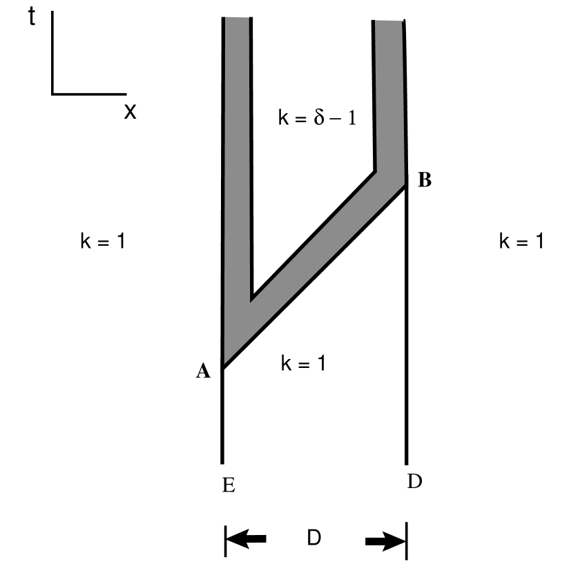
Figure 1: The Krasnikov spacetime in the $x-t$ plane. The vertical lines E and D are the world lines of the Earth and Deneb, respectively. The world line of the spaceship is (approximately) represented by the line AB.

The properties of the modified metric with $\delta-1\leq k\leq 1$ can be easily seen from the factored form of the expression for $ds^{2}$ in Eq. (4) where, putting $ds^{2}=0$, one sees that the two branches of the forward light cone in the $t,x$ plane are given by $dt/dx=1$, and $dt/dx=-k$. As $k$ becomes smaller and then negative, the slope of the left-hand branch of the light cone becomes less negative and then changes sign; i. e., the light cone along the negative $x$-axis “opens out”. This is illustrated in Fig. 2 where we depict the behavior of the light cone (in two spatial dimensions) for $k=1,\,k=0$, and $k=\delta-1$ for small $\delta$.

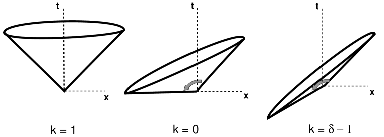
Figure 2: Forward light cones in the Krasnikov spacetime (illustrated with two space dimensions) for $k=1,\,k=0$, and $k=\delta-1$.

For $k\approx-1$, the boundary of the forward light cone is almost the straight line $x=t$, and the forward and backward light cones include almost all of spacetime.

In the internal region of Fig. 1, where $k=\delta-1=const$, space is flat, since the metric of Eq. (5) can be reduced to Minkowski form by the coordinate transformation

$$dt^{\prime} = dt+\left(\frac{\delta}{2}-1\right)\,dx\,,$$ (8)

$$dx^{\prime} = \left(\frac{\delta}{2}\right)\,dx\,.$$ (9)

Note that the left-hand branch of the light cone in the internal region is given in the Minkowski coordinates by $dt^{\prime}/dx^{\prime}=-1$, which, from Eqs. (8) and  (9), reduces to our previous expression $dt/dx=-k=1-\delta$ on the left-hand branch of the light cone as illustrated in Fig. 2. We also note that the transformation becomes singular at $\delta=0$, i. e., at $k=-1$.

From Eqs. (8) and  (9), we obtain

$$\frac{dt}{dt^{\prime}}=1+\left(\frac{2-\delta}{\delta}\right)\,\frac{dx^{\prime}}{dt^{\prime}}\,.$$ (10)

For an object propagating causally, i. e., into its forward light cone, we have $|dx^{\prime}/dt^{\prime}|<1$ and $dt^{\prime}>0$. Since $0<\delta\leq 2$, one sees that for such an object moving in the positive $x^{\prime}$ (and $x$) direction, $dt>0$ for any $\delta$. However, for $\delta<1$, an object moving sufficiently close to the left branch of the light cone given by $dx^{\prime}/dt^{\prime}=-1$, will have $dt/dt^{\prime}<0$ and thus appear to propagate backward in time as seen by observers in the external ($\delta=2\,,k=1$) region of Fig. 1. These properties of motion in the Krasnikov metric with $\delta<1$ can be seen from the shape of the light cone as shown in Fig. 2.

Now suppose our spaceship, having travelled from the Earth to Deneb and arriving at time $t\approx D$, has modified the metric so that $k\approx-1$ (i. e., $\delta\approx 0$) along its path. Suppose further that it now returns almost immediately to Earth, again travelling at a speed arbitrarily close to the speed of light as seen in its local inertial system, i. e., along the left-hand branch of the light cone with $dx^{\prime}/dt^{\prime}\approx-1$. It will then have $v_{r}\equiv dx/dt\approx-1/k=1/(1-\delta)\approx 1$ and $dt<0$ (since $dx<0$), and thus move down and to the left along the upper edge of the diagonal shaded region in Fig. 1. The spaceship’s return to Earth requires a time interval $\Delta t_{r}=-D/v_{r}=D(\delta-1)$, and the ship returns to Earth at a time $t_{E}$ as measured by clocks on the Earth given by $t_{E}=D+\Delta t_{r}=D\delta$. (For simplicity, here we treat the wall thickness, $\epsilon$, as negligible.)

Since $\delta>0$, $|\Delta t_{r}|<D$, and the spacetime interval between the spaceship’s departure from Deneb and its return to Earth is spacelike. Therefore the return journey must involve superluminal travel. Note that $t_{E}>0$, meaning that the return of the spaceship to Earth necessarily occurs after its departure. However, the interval between departure and return, as measured by observers on the Earth, can be made arbitrarily small by appropriate choice of the parameter $\delta$. The time of return, $t_{E}$ must necessarily be positive, since causality insures that the metric is modified, opening out the light cone to allow causal propagation in the negative $t$-direction, only for $t>0$. Since $t_{E}>0$, the spaceship cannot travel into its own past; i. e., the metric of Ref.[12], as it stands, does not lead to CTCs and the existence of a time machine. However, when the metric  (5) is generalized to the more realistic case of three space dimensions CTCs do become possible, as we shall see below.

Before turning to the three dimensional generalization, we note one other interesting property of the Krasnikov metric. In the case $\delta<1$, it is always possible to choose an allowed value of $dx^{\prime}/dt^{\prime}$ for which $dt/dt^{\prime}=0$, meaning that the return trip is instantaneous as seen by observers in the external region of Fig. 1. This can be seen from the third diagram in Fig. 2. It also follows easily from Eq. (10), which implies that $dt/dt^{\prime}=0$ when $dx^{\prime}/dt^{\prime}$ satisfies

$$\frac{dx^{\prime}}{dt^{\prime}}=-\frac{\delta}{(2-\delta)}\,,$$ (11)

which lies between $0$ and $-1$ for $0<\delta<1$.

3 Generalization to Four Dimensions

In four dimensions the modification of the metric begins along the path of the spaceship, i. e., the $x$-axis, occurring at position $x$ at time $t\approx x$, the time of passage of the spaceship. We assume that the disturbance in the metric propagates radially outward from the $x$-axis, so that causality guarantees that at time $t$ the region in which the metric has been modified cannot extend beyond $\rho=t-x$, where $\rho={(y^{2}+z^{2})}^{1/2}$. It also seems natural to take the modification in the metric not to extend beyond some maximum radial distance $\rho_{max}\ll D$ from the $x$-axis. Thus in four dimensional spacetime we replace Eq. (6) by

$$k(t,x,\rho)\equiv 1-(2-\delta)\,\theta_{\epsilon}(\rho_{max}-\rho)\,\theta_{\epsilon}(t-x-\rho)\,[\theta_{\epsilon}(x)-\theta_{\epsilon}(x+\epsilon-D)]\,,$$ (12)

and our metric, now written in cylindrical coordinates, is given by

$$ds^{2}=-dt^{2}+(1-k(t,x,\rho))\,dx\,dt+k(t,x,\rho)\,dx^{2}+d{\rho}^{2}+{\rho}^{2}\,d{\phi}^{2}\,.$$ (13)

(Again we assume for simplicity that the $\epsilon$-parameters in all of the $\theta_{\epsilon}$-functions which appear in the expression for $k$ are equal.) For $t\gg D+\rho_{max}$ one now has a tube of radius $\rho_{max}$ centered on the $x$-axis within which the metric has been modified; we refer to this structure as a “Krasnikov tube”. In contrast with the metric of Ref.[1], the metric of a Krasnikov tube is static once it has been initially created. If we make the assumption that $\rho_{max}\gg\epsilon$, such a tube will consist of a relatively large central core, of radius $\rho_{max}-\epsilon$, along the $x$-axis with $\epsilon<x<D-\epsilon$; within this central core space is flat and $k=\delta-1=const$. This central core will be surrounded by thin walls and end caps of thickness $\epsilon$, within which there is curved space with $k$ varying between $k=\delta-1$ and $k=1$. The situation is illustrated in Fig. 3, which shows cross-sections through the tube in the region $\epsilon<x<D-\epsilon$ and also in one of the end caps.

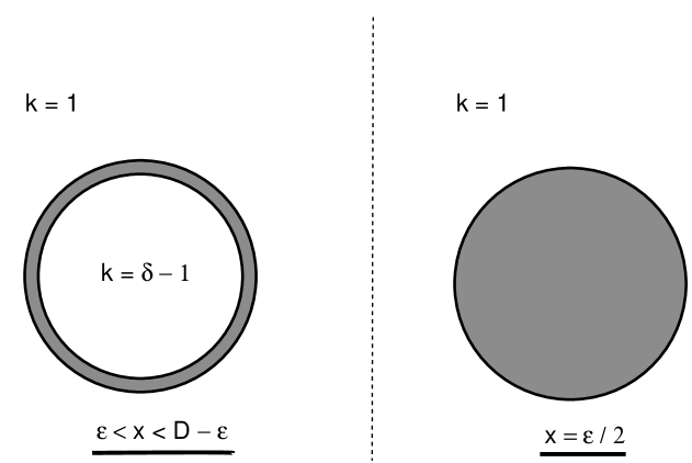
Figure 3: Spatial cross-sections of a Krasnikov tube at $x=const$, $t=const$. The left diagram represents a cross-section through the middle of the tube between the end caps, while the right diagram is a cross-section through an end cap.

4 A Superluminal Subway and Closed Timelike Curves

As we have seen, in two dimensions a single Krasnikov tube allows superluminal travel backward in $t$ in one direction along the $x$-axis, and does not lead to CTCs. However, in three space dimensions the situation is different. Assuming that Krasnikov tubes can be established, imagine that a spaceship has travelled from the Earth to Deneb along the $x$-axis during the time interval from $t=0$ to $t=D$, and established the Krasnikov tube running from the Earth to Deneb which we have discussed. It would then be possible for the ship to return from Deneb to the Earth outside the first tube along a path parallel to the $x$-axis but at a distance $\rho_{0}$ from it, where $D\gg\rho_{0}>2\rho_{max}$. On the return journey the spaceship crew could again modify the metric along their path, establishing a second Krasnikov tube identical to the first but running in the opposite direction; that is, the metric within the second tube would be given by that of Eq. (13) with $x$ replaced by $X\equiv D-x$ and $t$ replaced by $T\equiv t-D$. The crucial point is that in three dimensions the two tubes can be made non-overlapping because of their separation in the $\rho$-direction. The spaceship can now, for example, start from the Earth ($x=0$) at $t=2D$, and travel back in time to the Earth at a time arbitrarily close to $t=0$ by first using the second Krasnikov tube to travel to Deneb ($x=D$) at time $t=D$, and then using the original tube as before, to travel from Deneb at $t=D$ to the Earth at $t=0$. (We are assuming that the ship travels at essentially light speed, that $\delta$ and $\epsilon$ are taken to be negligibly small, and that the small time required to move the distance $\rho_{0}\ll D$ from one of the Krasnikov tubes to the other is negligible.) It may be worth noting that the foregoing argument is closely analogous to that given in Ref.[3] for the existence of CTCs in the Alcubierre case. The situation is also similar to the case of time travel using a two-wormhole system, as depicted in the spacetime diagram of Fig. 18.5 of Ref.[14].

It follows from the foregoing discussion that if Krasnikov tubes could be constructed, one could, at least in principle, establish a network of such tubes forming a sort of interstellar subway system allowing instantaneous communication between points connected by the tubes. A necessary corollary of the existence of such a network is the possibility of backward time travel and the consequent existence of CTCs. CTCs could be avoided only if, for some reason, there existed a preferred axis such that all the Krasnikov tubes were oriented so that the velocity components along that axis of objects in superluminal motion were always positive, implying that no object could return to the same point in time and space. One might be tempted to reject immediately the possibility of Krasnikov tubes for interstellar travel because, unlike Alcubierre bubbles, their required length would be enormous. However, there are interesting situations in astronomy, e. g., jets in active galactic nuclei and possibly cosmic strings, which involve (albeit positive) matter distributions of such dimensions. In any event, even if the construction of Krasnikov tubes over astronomical distances is impractical, oppositely directed non-overlapping pairs of tubes of laboratory dimensions could form time machines, forcing one to confront all the associated problems.

5 The Stress-Energy Tensor for a Krasnikov Tube

In this section, we show that the WEC is necessarily violated in some regions of a Krasnikov tube. The stress-energy tensor $T_{\mu\nu}$ for the matter needed to produce a Krasnikov tube can be calculated from the metric of Eq. (13) and the Einstein equations, using the program MATHTENSOR [15]. We first obtain an expression for $T_{\mu\nu}$ in terms of derivatives of $k$ with respect to the spacetime coordinates. The stress tensor element $T_{tt}$ is given by the following expression:

$$T_{tt}={\left[{32\,\pi\,{(1+k)}^{2}}\right]}^{-1}\,\biggl{[}{\frac{-4\,(1+k)}{\rho}\,\frac{\partial k}{\partial\rho}\,+\,3{\biggl{(}\frac{\partial k}{\partial\rho}\biggr{)}}^{2}\,-\,4\,(1+k)\,\frac{{\partial}^{2}k}{{\partial\rho}^{2}}}\biggr{]}\,.$$ (14)

(It will be shown later that this is the energy density seen by a static observer.) Note that this component of the stress tensor involves only derivatives of $k$ with respect to $\rho$. A number of general features of the $k$ vs. $\rho$ curve illustrated in Fig. 4 are generic and follow from Eq. (12) without specifying an explicit form for $\theta_{\epsilon}$.

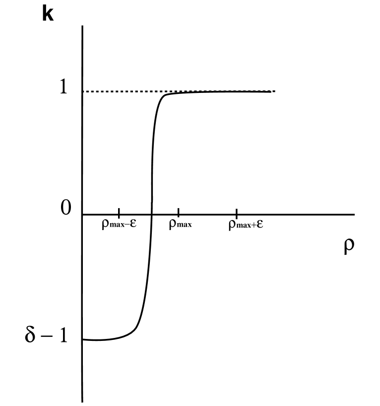
Figure 4: Graph of $k$ vs $\rho$ at constant $x,t$. Here $\epsilon<x<D-\epsilon$.

In particular, $k$ increases monotonically from its value at $\rho=0$ to $k\approx 1$ at $\rho\geq\rho_{max}$, so that $\partial k/\partial\rho$ and $(1+k)$ are positive. Furthermore, analyticity of $k$ at $\rho=0$ implies that $\partial k/\partial\rho$ vanishes at that point. From the previous remarks, we have that $\partial k/\partial\rho\approx\beta{\rho}^{m}$, with $m\geq 1$, $\beta>0$, for small $\rho$. Hence, sufficiently near the axis of the Krasnikov tube, the first and third terms on the right-hand side of Eq. (14) are negative and go as ${\rho}^{m-1}$ for $\rho\rightarrow 0$; these terms thus dominate the second term, which is positive, by a factor of ${\rho}^{-m-1}$. Therefore there is necessarily a range of $\rho$ near the axis of the tube where the energy density seen by a static observer is negative.

As we have noted previously, for a thin-walled tube, space is nearly flat and so $T_{tt}\approx 0$ within the core of the tube. Thus in the region near $\rho=0$ where we can make a general statement about the sign of $T_{tt}$ on the basis of the preceding argument, we expect $T_{tt}$ to be extremely small due to the behavior of the function $\theta_{\epsilon}(\rho_{max}-\rho)$. (We observe that the case $k=-1$, corresponding to $\delta=0$, is not allowed, since that would produce a divergence in $T_{tt}$.) In the vicinity of the tube wall, where $T_{tt}$ is large, we can only obtain its value by choosing an explicit form for $k$, i. e., for $\theta_{\epsilon}$, and then evaluating $T_{tt}$ numerically. In Fig. 5 we show a plot of $T_{tt}$ in the region of the tube wall obtained in this way, using the form of $\theta_{\epsilon}$ given in the next section, and taking $x=D/2$, $t\gg\rho_{max}+D/2$, and $\epsilon/\rho_{max}\ll 1$.

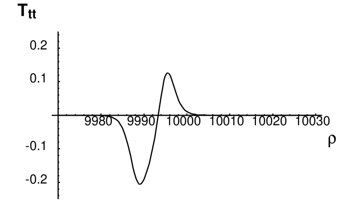
Figure 5: Graph of energy density vs. $\rho$ at the middle of the tube, i. e., at $x=D/2$ and $t=const\gg D/2+\rho_{max}$. Here we have chosen $\delta=0.01,\,\epsilon=10$, and $\rho_{max}=1000\,\epsilon$. The plot extends from $\rho_{max}-3\epsilon$ to $\rho_{max}+3\epsilon$.

We see that $T_{tt}$ is negative on the inner side of the wall, as one would expect, since the general argument given above shows that $T_{tt}$ must be negative for small $\rho$. However, $T_{tt}$ changes sign and develops appreciable positive values on the outer side of the wall. The corresponding plot at $x=\epsilon/2$, in the left endcap, is very similar to Fig. 5. There are two main differences: first, the magnitudes of the positive and negative energy density maximum and minimum are essentially equal; and second, these magnitudes are roughly four times smaller than at $x=D/2$.

6 Quantum Inequality Constraints

In Ref.[8], an inequality was proven which limits the magnitude and duration of the negative energy density seen by an inertial observer in Minkowski spacetime. Let $\langle T_{\mu\nu}\rangle$ be the renormalized expectation value of the stress tensor for a free, massless, minimally coupled scalar field in an arbitrary quantum state. Let $u^{\mu}$ be the observer’s four-velocity, so that $\langle T_{\mu\nu}u^{\mu}u^{\nu}\rangle$ is the expectation value of the local energy density in this observer’s frame of reference. The inequality states that

$${{\tau_{0}}\over\pi}\,\int_{-\infty}^{\infty}\,{{\langle T_{\mu\nu}u^{\mu}u^{\nu}\rangle\,d\tau}\over{{\tau}^{2}+{\tau_{0}}^{2}}}\geq-{3\over{32{\pi}^{2}{\tau_{0}}^{4}}}\,,$$ (15)

for all $\tau_{0}$, where $\tau$ is the observer’s proper time. The Lorentzian function which appears in the integrand is a convenient choice for a sampling function, which samples the energy density in an interval of characteristic duration $\tau_{0}$ centered around an arbitrary point on the observer’s worldline. The proper time coordinate has been chosen so that this point is at $\tau=0$. Physically, Eq. (15) implies that the more negative the energy density is in an interval, the shorter must be the duration of the interval. Such a bound is called a “quantum inequality” (QI). (More recently, a much simpler proof of Eq. (15) has been given, as well as derivations of similar bounds for the massive scalar and electromagnetic fields [10].)

Although the QI-bound was initially derived for a massless scalar field in Minkowski spacetime (without boundaries), it was argued in Ref.[9] that in fact the bound should also hold in a curved spacetime and/or one with boundaries, in the limit of short sampling times. More specifically, when the sampling time $\tau_{0}$ is restricted to be smaller than the smallest proper radius of curvature or the distance to any boundaries, then the modes of the quantum field may be approximated by plane waves, i.e., spacetime is approximately Minkowski. In this region, Eq. (15) should hold. Further evidence supporting this conclusion has recently appeared in the form of QI-bounds which have been explicitly proven in various static curved spacetimes. In all cases, these bounds reduce to the flat spacetime QI’s in the short sampling time limit [16, 17].

In Ref.[9] the flat spacetime bound was applied, in the limit of short sampling times, to Morris-Thorne traversable wormhole spacetimes. The upshot of the analysis was that either the wormhole throat could be no larger than a few times the Planck length, or there must be large discrepancies in the length scales which characterize the wormhole. In the latter case, this typically implied that the exotic matter which maintains the wormhole geometry must be concentrated in an exceedingly thin band around the throat. These results would appear to make the existence of static traversable wormholes very unlikely. A similar analysis using the flat space QI has been applied to the Alcubierre “warp drive” spacetime [11], which also requires exotic matter. Here as well, it was found that the wall of the “warp bubble” surrounding a spaceship must be unphysically thin compared to the bubble radius. In this section, we apply the flat space QI to the Krasnikov spacetime, again in the short sampling time limit, and reach a similar conclusion regarding the thickness of the negative energy regions of the Krasnikov tube.

Consider a geodesic observer who is initially at rest, i.e., $dx/d{\tau}=d{\rho}/d{\tau}=d{\phi}/d{\tau}=0$. These initial conditions imply

$$\frac{d^{2}x^{\mu}}{{d\tau}^{2}}+\Gamma^{\mu}_{\,\,tt}\,\biggl{(}\frac{dt}{d\tau}\biggr{)}^{2}\,=0\,,$$ (16)

which reduce to:

$$\frac{d^{2}t}{{d\tau}^{2}}-\frac{(1-k)\,{k,_{t}}}{(1+k)^{2}}\,\biggl{(}\frac{dt}{d\tau}\biggr{)}^{2}\,=0\,,$$ (17)

$$\frac{d^{2}x}{{d\tau}^{2}}-\frac{2\,{k,_{t}}}{(1+k)^{2}}\,\biggl{(}\frac{dt}{d\tau}\biggr{)}^{2}\,=0\,,$$ (18)

$$\frac{d^{2}\rho}{{d\tau}^{2}}\,=\,\frac{d^{2}\phi}{{d\tau}^{2}}\,=0\,.$$ (19)

Therefore we see that initially static geodesic observers will remain static in the region of the spacetime where $k,_{t}\equiv\partial k/{\partial t}=0$, i.e., long after the formation of the tube. In this region, from Eq. (17), $dt/{d\tau}=const$, which we could choose to be $1$ so that $dt=d\tau$. By suitably adjusting the zeros of each time coordinate, we can make the coordinate time, $t$, equal to the proper time, $\tau$, in this region.

To apply the flat spacetime QI, we must first transform to the orthonormal frame of the static geodesic observer. The metric, Eq. (13), can be diagonalized by the transformation

$$d{\hat{t}} = dt-\biggl{(}\frac{1-k}{2}\biggr{)}\,dx\,,$$ (20)

$$d{\hat{x}} = \biggl{(}\frac{1+k}{2}\biggr{)}\,dx\,,$$ (21)

$$d{\hat{\rho}} = d\rho\,$$ (22)

$$d{\hat{\phi}} = \rho\,d\phi\,,\$$ (23)

which corresponds to the (non-coordinate) basis [18]

$${\bf e}_{\hat{t}} = {\bf e}_{t}\,,$$ (24)

$${\bf e}_{\hat{x}} = \biggl{(}\frac{1-k}{1+k}\biggr{)}\,{\bf e}_{t}\,+\,\biggl{(}\frac{2}{1+k}\biggr{)}\,{\bf e}_{x}\,,$$ (25)

$${\bf e}_{\hat{\rho}} = {\bf e}_{\rho}\,,$$ (26)

$${\bf e}_{\hat{\phi}} = \biggl{(}\frac{1}{\rho}\biggr{)}\,{\bf e}_{\phi}\,.$$ (27)

In this basis, using the fact that ${\bf e}_{\alpha}\cdot{\bf e}_{\beta}=g_{\alpha\beta}$, we have

$${\bf e}_{\hat{\mu}}\cdot{\bf e}_{\hat{\nu}}=\eta_{\hat{\mu}\hat{\nu}}\,.$$ (28)

It is also easily seen that, in the region where $k=1$, Eqs. (24-27) reduce to a set of orthonormal basis vectors in ordinary Minkowski spacetime. (Note that this basis is also well-behaved in the case when $k=0$.)

The stress-tensor and Riemann tensor components in this frame are

$$T_{\hat{\mu}\hat{\nu}}=T_{ab}\,e^{a}_{\hat{\mu}}\,e^{b}_{\hat{\nu}}\,,$$ (29)

and

$$R_{\hat{\mu}\hat{\nu}\hat{\alpha}\hat{\beta}}=R_{abcd}\,e^{a}_{\hat{\mu}}\,e^{b}_{\hat{\nu}}\,e^{c}_{\hat{\alpha}}\,e^{d}_{\hat{\beta}}\,,$$ (30)

respectively. Here the greek indices label the vector of the basis, and the latin indices denote components in the original (coordinate) frame. From Eqs. (24) and  (29), we see that the energy density in the orthonormal frame is the same as in the coordinate frame, i.e.,

$$T_{\hat{t}\hat{t}}=T_{tt}\,.$$ (31)

We will evaluate the energy density in the middle of the left end cap at a time long after the formation of the tube, i.e., at $x=\epsilon/2,\,t\gg x+\rho+\epsilon$. In this region

$$\theta_{\epsilon}(x+\epsilon-D)=0\,,$$ (32)

and

$$\theta_{\epsilon}(t-x-\rho)=1\,.$$ (33)

Therefore, in our chosen region, we have

$$k=1-(2-\delta)\,\theta_{\epsilon}(\rho_{max}-\rho)\,\theta_{\epsilon}(x)\,.$$ (34)

Let us now choose the following specific form for $\theta_{\epsilon}(\xi)$ :

$$\theta_{\epsilon}(\xi)=\frac{1}{2}\,\biggl{\{}{\rm tanh}\biggl{[}2\,\biggl{(}\frac{2\xi}{\epsilon}-1\biggr{)}\biggr{]}+1\biggr{\}}\,.$$ (35)

This function has the general desired properties outlined in Sec. 3 [19]. However, we do not expect our main conclusion to depend on the detailed form of $k$. At $x=\epsilon/2$, $\theta_{\epsilon}(x)=0.5$, so

$$k = 1-\biggl{(}1-\frac{\delta}{2}\biggr{)}\,\theta_{\epsilon}\,(\rho_{max}-\rho)$$ (36)

$$= 1-\frac{1}{2}\,\biggl{(}1-\frac{\delta}{2}\biggr{)}\,\biggl{\{}{\rm tanh}\biggl{[}2\,\biggl{(}\frac{2(\rho_{max}-\rho)}{\epsilon}-1\biggr{)}\biggr{]}+1\biggr{\}}\,.$$ (37)

Note that from Eq. (14), the energy density depends only on derivatives of $k$ with respect to $\rho$. Consider a static observer in the middle of the left end cap at $\rho=\rho_{max}-\epsilon$. Let $\rho_{max}=n\epsilon$, where $n>1$, although $n$ is not necessarily assumed to be an integer. Substitution of these expressions into Eq. (14) gives [20]

$$T_{\hat{t}\hat{t}}=\biggl{(}\frac{1}{8\pi}\biggr{)}\,\frac{[0.271\,(3.504-4.034\,n-0.008\,\delta+0.017\,n\,\delta-0.872\,{\delta}^{2}+n\,{\delta}^{2})]}{{\epsilon}^{2}\,(n-1)\,{(1.018+0.491\,\delta)}^{2}}\,.$$ (38)

Recall that $0\mathrel{\raise 1.29167pt\hbox{$<$\kern-7.5pt\lower 4.30554pt\hbox{$\sim$}}}\delta\leq 2$. The value $\delta=2$ corresponds to $k=1$ (usual Minkowski spacetime with no opening of the light cone), while $\delta\approx 0$ corresponds to $k\approx-1$ in the vacuum inside the tube (Minkowski spacetime with maximum “opening out” of the light cone). Therefore, for effective “warp travel”, we want $\delta$ to be as small as possible. Expansion of Eq. (38) in a power series in $\delta$ shows that for small $\delta$ and $n$ large compared to $1$,

$$T_{\hat{t}\hat{t}}\approx-\frac{1}{8\pi{\epsilon}^{2}}\,.$$ (39)

Let the magnitude of the maximum curvature tensor component in the static orthonormal frame be denoted by $\hat{R}_{max}$. Then a (somewhat tedious) calculation using Eq. (30) shows that for our chosen observer, in the same limits,

$$\hat{R}_{max}\approx\frac{1}{{\epsilon}^{2}}\,.$$ (40)

(Note that the curvature tensor components, unlike the energy density, will contain derivatives of $k$ with respect to $x$.) Hence the smallest proper radius of curvature at this location is

$$r_{c}\approx\frac{1}{\sqrt{\hat{R}_{max}}}\approx\epsilon\,.$$ (41)

Let us now apply the QI-bound, Eq. (15), to the energy density seen by our static geodesic observer. We assume that $T_{\hat{t}\hat{t}}$ is the expectation value of the stress-tensor operator in some quantum state of the quantized massless scalar field [21]. As argued previously in Ref.[9], for this flat spacetime bound to be applicable, we must restrict our sampling time to be smaller than the smallest local proper radius of curvature, i.e.,

$$\tau_{0}=\sigma\,\epsilon\,,$$ (42)

where $\sigma\ll 1$. In this region, spacetime is approximately flat. Note that as long as we consider the region of spacetime corresponding to times long after tube formation, the limit of short sampling times should also kill off any effects of time-dependence of the metric, which occurred during tube formation, on the modes of the quantum field. Over the timescale $\tau_{0}$, the energy density is approximately constant, so we have

$${{\tau_{0}}\over\pi}\,\int_{-\infty}^{\infty}\,{{T_{\hat{t}\hat{t}}\,\,d\tau}\over{{\tau}^{2}+{\tau_{0}}^{2}}}\approx\,T_{\hat{t}\hat{t}}\,\mathrel{\raise 1.29167pt\hbox{$>$\kern-7.5pt\lower 4.30554pt\hbox{$\sim$}}}-{3\over{32{\pi}^{2}{\sigma}^{4}{\epsilon^{4}}}}\,,$$ (43)

which implies

$$\epsilon\mathrel{\raise 1.29167pt\hbox{$<$\kern-7.5pt\lower 4.30554pt\hbox{$\sim$}}}\frac{l_{P}}{{\sigma}^{2}}\,,$$ (44)

where $l_{P}$ is the Planck length. For a “reasonable” choice of $\sigma$, for example $\sigma\approx 0.01$, we have that

$$\epsilon\mathrel{\raise 1.29167pt\hbox{$<$\kern-7.5pt\lower 4.30554pt\hbox{$\sim$}}}10^{4}\,l_{P}\approx 10^{-31}\,{\rm m}\,.$$ (45)

For an observer in the middle of the right end cap, i. e., at $x=D-\epsilon/2$, it is easily shown that the expression for $k$ is the same as that given in Eq. (37). Since the energy density depends only on derivatives of $k$ with respect to $\rho$, its value will be the same for observers in the middle of each end cap, at the same $\rho$-position. For times long after tube formation, the spacetime is spatially symmetric with respect to reflections of the tube through the plane $x=D/2$. Hence the components of the curvature tensor in the static orthonormal frame should be the same at $x=\epsilon/2$ and $x=D-\epsilon/2$. Therefore our previous argument should apply to both end caps.

At the midpoint of the tube, i. e., at $x=D/2$, $\theta_{\epsilon}(x)=1$ and $\theta_{\epsilon}(x+\epsilon-D)=0$, so in the static region $k=1-(2-\delta)\,\theta_{\epsilon}(\rho_{max}-\rho)$. One can again show that for a static observer at $\rho=\rho_{max}-\epsilon$, $T_{\hat{t}\hat{t}}\approx-1/(8\pi{\epsilon}^{2})$, in the small $\delta$ limit. (The nonzero energy density in the region just inside the inner wall of the tube is a consequence of the “tails” of the $\theta_{\epsilon}$-functions.) By symmetry, in this region, $k,_{x}=0$ at $x=D/2$. It can be shown that the curvature tensor components contain no second derivatives with respect to $x$. The components can therefore only depend on derivatives of $k$ with respect to $\rho$. Again one can show that the smallest proper radius of curvature at this location is $r_{c}\approx\epsilon$. Therefore our conclusion, Eq. (45), applies to the walls of the (hollow) Krasnikov tube as well as to the end caps [22].

In the preceding discussion, we assumed that $\rho_{max}\gg\epsilon$, i. e., that $n$ was large compared to $1$. If we relax this requirement and consider thick tubes, with $n$ of order $1$, then $\rho_{max}\approx\epsilon$. In this case, from dimensional arguments, we should have $T_{\hat{t}\hat{t}}\approx-1/(8\pi\,{\rho_{max}}^{2})$, $\hat{R}_{max}\approx 1/{\rho_{max}}^{2}$, and $r_{c}\approx\rho_{max}$. Application of our QI now yields a bound on the radius of the tube:

$$\rho_{max}\mathrel{\raise 1.29167pt\hbox{$<$\kern-7.5pt\lower 4.30554pt\hbox{$\sim$}}}\frac{l_{P}}{{\sigma}^{2}}\,.$$ (46)

This result is similar to that found in the case of traversable wormholes.

Let us now estimate the total amount of negative energy required for the maintenance of a Krasnikov tube [23]. Our task is complicated by the fact that the $t=const$ slices of the Krasnikov spacetime are not everywhere spacelike. The metric on such a slice is given by

$$ds^{2}=k(t,x,\rho)\,dx^{2}+d{\rho}^{2}+{\rho}^{2}\,d{\phi}^{2}\,,$$ (47)

which can be nonspacelike when $k<0$. Therefore let us instead estimate the total negative energy in a thin band in $\rho$ over which $k\approx const$. In this band, from Eqs. (20) and  (21), the metric can be written as

$$ds^{2}=-d{\hat{t}}^{2}\,+d{\hat{x}}^{2}\,+d{\rho}^{2}\,+{\rho}^{2}\,d{\phi}^{2}\,.$$ (48)

Consider a band $\Delta\rho$ where $k\approx const$ and the energy density is most negative. We see from Fig. 5 that such a band has the form

$$\Delta\rho=\alpha\epsilon\,,$$ (49)

where $\alpha\ll 1$. For a small enough choice of $\alpha$, we can write the metric in this region in the simple form, Eq. (48). The proper volume of the band is

$$V\approx 2\pi\rho_{max}\,(\Delta\rho)\,D=2\pi\alpha\epsilon\,\rho_{max}\,D\,.$$ (50)

A rough estimate of the total negative energy contained in this band is

$$E\approx T_{\hat{t}\hat{t}}\,V\approx-\frac{\alpha\,\rho_{max}\,D}{\epsilon}\,.$$ (51)

From our QI bound, Eq. (44), we also have that $\epsilon\approx l_{P}/{\sigma}^{2}$, where $\delta$ is assumed to be very small. As an example, let $D=\rho_{max}=1\,{\rm m}=10^{35}\,l_{P}$, and $\epsilon=100\,l_{P}$. Then

$$E\approx-\alpha\,10^{68}\,m_{Planck}=-\alpha\,10^{63}\,{\rm g}=-\alpha\,10^{18}\,M_{galaxy}\,,$$ (52)

where we have taken $M_{galaxy}\approx 10^{12}$ solar masses. Thus even if we take $\alpha$ to be very small, say $0.01$, one requires negative energies of the order of $10^{16}$ galactic masses just to make a Krasnikov tube $1$ meter long and $1$ meter wide. For a tube that stretches from here to the nearest star, i. e. $D\approx 4\times 10^{16}{\rm m}$, we need $E\approx-10^{32}M_{galaxy}$. Similar orders of magnitude were found in the case of the Alcubierre warp bubble [11]. Note that we do not expect the positive and negative energies on the outside and inside of the tube to add to zero in general, since the cancellation would have to be exact to extraordinarily high accuracy [24], given the large magnitudes involved.

We have been assuming that $\delta\approx 0$, so as to maximize the amount by which the light cone is opened out within the tube. In particular, values of $\delta<1$ are needed to allow travel backward in time and the possibility of CTCs. The dependence of our results on $\delta$ can be easily estimated as follows. Define $\eta=2-\delta$, so that $k=1-\eta$ within the (hollow part of the) tube, and $k$ changes by $\eta$ across the wall of the tube. For $k=1-\eta$, the left-hand branch of the light cone in Fig. 2 is given by $dx/dt=-1/(1-\eta)$. We see that $\partial k/\partial\rho\sim\eta/\epsilon$ and ${\partial}^{2}k/\partial{\rho}^{2}\sim\eta/{\epsilon}^{2}$ within the tube wall; thus, from Eq. (14), in the limit $\eta\ll 1$ and $\epsilon\ll\rho$, $T_{tt}$ scales as $\eta/{\epsilon}^{2}$, and $r_{c}\gg\epsilon$. For small $\eta$, the negative energy densities in the walls are thus very small and the QI bound, as well as the requirement $\tau_{0}\ll r_{c}$, can be satisfied for macroscopic values of $\epsilon$ and $\tau_{0}$. For example, one can satisfy the QI with $\tau_{0}=\epsilon\approx 1\,{\rm cm}$, but only by taking $\eta\approx{l_{P}}^{2}\,{\epsilon}^{2}/{\tau_{0}}^{4}\approx 10^{-66}$. It might therefore actually be possible to establish a region within which superluminal travel is, in principle, allowed. However the change in the slope of the left branch of the light cone, illustrated in Fig. 2, is proportional to $\eta$ for small $\eta$, and hence the speed of a light ray directed along the negative $x$-axis within the tube, as seen by observers outside, would exceed $1$ by only one part in $10^{66}$. The existence of superluminal travel would thus appear to be completely unobservable.

7 Conclusions

The Alcubierre “warp drive” spacetime suffers from the drawback that a spaceship at the center of the warp bubble is causally disconnected from the outer wall of the bubble. We have discussed and generalized a metric, originally designed by Krasnikov to circumvent this problem, which requires that any modification of the spacetime to allow superluminal travel necessarily occurs in the causal future of the launch point of the spaceship. As a result, this metric has the interesting feature that the time for a one-way trip to a distant star is limited by all the usual restrictions of special relativity, but the time for a round trip may be made arbitrarily short. In four dimensions this entails the creation of a “tube” during the outbound flight of the spaceship, which connects the Earth and the star. Inside the tube, the spacetime is flat but with the light cones “opened out” to allow superluminal travel in one direction, as seen by observers outside the tube. Although the creation of a single Krasnikov tube does not entail the formation of closed timelike curves, we showed that two spatially separated tubes could be used to construct a time machine - a feature shared by two-wormhole or two-warp bubble systems. This poses a problem for causality even if tubes of only, say, laboratory dimensions could be realized in practice.

In addition, we have also shown that, with relatively modest assumptions, maintenance of a such a tube long after formation will necessarily require regions of negative energy density which can be no thicker than a few thousand Planck lengths. Estimates of the total negative energy required to construct Krasnikov tubes of even modest dimensions were shown to be unphysically large. Similar difficulties have been recently shown to plague warp bubbles and wormholes [25]. The Krasnikov tube suffers from some of the same drawbacks as these other proposed methods of faster-than-light travel, and is hence also a very unlikely possibility.

Acknowledgements

We would like to thank Michael Pfenning and Larry Ford for helpful discussions. TAR would like to thank the members of the Tufts Institute of Cosmology for their gracious hospitality while this work was being done. This research was supported in part by NSF Grant No. PHY-9507351 and by a CCSU/AAUP faculty research grant.

References

- [1] M. Alcubierre, Class. Quantum Grav. 11, L73 (1994).
- [2] S.W. Hawking and G.F.R. Ellis, The Large Scale Structure of Spacetime (Cambridge University Press, London, 1973), p. 88-96.
- [3] A. Everett, Phys. Rev. D 53, 7365 (1996).
- [4] M. Morris, K. Thorne, and Y. Yurtsever, Phys. Rev. Lett. 61, 1446 (1988).
- [5] S.W. Hawking, Phys. Rev. D 46, 603 (1992).
- [6] H. Epstein, V. Glaser, and A. Jaffe, Nuovo Cim. 36, 1016 (1965).
- [7] C. Kuo, “A Revised Proof of the Existence of Negative Energy Density in Quantum Field Theory”, gr-qc/961104, to appear in Nuovo Cimento Il.
- [8] L.H. Ford and T.A. Roman, Phys. Rev. D 51, 4277 (1995).
- [9] L.H. Ford and T.A. Roman, Phys. Rev. D 53, 5496 (1996).
- [10] L.H. Ford and T.A. Roman, “Restrictions on Negative Energy Density in Flat Spacetime”, gr-qc/9607003, Phys. Rev. D, to appear.
- [11] M. Pfenning and L.H. Ford, “The Unphysical Nature of ‘Warp Drive’ ”, gr-qc/9702026.
- [12] S.V. Krasnikov, “Hyper-Fast Interstellar Travel in General Relativity”, gr-qc/9511068.
- [13] A similar argument has been given by M. Pfenning (unpublished).
- [14] M. Visser, Lorentzian Wormholes - from Einstein to Hawking (American Institute of Physics Press, New York, 1995).
- [15] L. Parker and S.M. Christensen, MathTensor (MathSolutions, Inc., Chapel Hill, NC, 1992).
- [16] M. Pfenning and L.H. Ford, “Quantum Inequalities on the Energy Density in Static Robertson-Walker Spacetimes”, Tufts University preprint, gr-qc/9608005, to appear in Phys. Rev. D.
- [17] M. Pfenning and L.H. Ford, unpublished.
- [18] See, for example, Sec. 5.6 of B. Schutz, A First Course in General Relativity (Cambridge Univ. Press, 1985).
- [19] The specific form of chosen here has the minor drawback that the numerical value of does not quite go exactly to zero at (as it must by symmetry), although it does become very small. The resulting apparent “singularity” in at can be remedied by using a somewhat more cumbersome form of with an additional term which has the effect of forcing at . Since this added complication changes neither our results nor our conclusion, while tending to obscure the physical interpretation of , we have chosen to use the simpler form.
- [20] The apparent singularity in when is related to the problem at mentioned in the previous footnote. It arises because for , we are evaluating at .
- [21] From the results of Ref.[10], our conclusion will be the same if we construct the Krasnikov tube out of quantized massive scalar or electromagnetic fields.
- [22] We assumed for simplicity that the values of the ’s in all of the -functions were equal. Relaxation of this assumption would make the model more complicated but should not, we believe, change the essential result. That is, in the latter case as well, we expect that (although we have not proven it) at least one of the ’s appearing in the expression for will be constrained by the quantum inequality to be exceedingly small.
- [23] Of course the total energy (matter plus gravitational) of the Krasnikov tube, as measured by observers at infinity, is zero since the external metric is Minkowskian.
- [24] The authors are grateful to Larry Ford for suggesting several key parts of this argument.
- [25] The problem of the total amount of negative energy required is not quite as severe in the case of wormholes. For example, for an “absurdly benign” wormhole, discussed in Ref. [9], the energy density is equal to , where is the thickness of the negative energy band and is the throat radius. The proper volume is approximately ; hence the total negative energy required is . However, this still requires about one Jupiter mass of negative energy to support a wormhole with a meter throat radius (see p. 174 of Ref. [14]). In the cases of the Alcubierre bubble and the Krasnikov tube, the negative energy density scales as , so the total negative energy required scales as , where is the thickness of the wall.