Stationary Bianchi type II perfect fluid models

Abstract

Einstein’s field equations for stationary Bianchi type II models with a perfect fluid source are investigated. The field equations are rewritten as a system of autonomous first order differential equations. Dimensionless variables are subsequently introduced for which the reduced phase space is compact. The system is then studied qualitatively using the theory of dynamical systems. It is shown that the locally rotationally symmetric models are not asymptotically self-similar for small values of the independent variable. A new exact solution is also given.

PACS number(s): 04.20.-q, 04.20.Jb, 04.40.Nr, 95.30.Sf

I Introduction

Dynamical systems methods have been used for over 20 years for studying the behavior of different models in general relativity, especially in the field of cosmology, see e.g. [1]. The dynamical systems approach constitute a powerful tool when one wants to study asymptotic and intermediate behavior. It allows one to obtain a good understanding of the models even though it may be impossible to solve the corresponding equations exactly. Most of the attractors in the cosmological context have turned out to be self-similar solutions but there are also more exotic ones, e.g. the Mixmaster attractor. In this article we will apply the dynamical systems approach to the stationary Bianchi type II models. It will be shown that the locally rotationally symmetric (LRS) models are not asymptotically self-similar for small values of the independent variable. Instead the attractor is described by a heteroclinic cycle. To our knowledge, the stationary LRS type II models yield the simplest example of a non-self-similar attractor in general relativity.

We will consider Bianchi type II models which admit a simply transitive group of isometries acting on 3-dimensional hypersurfaces which are timelike. The line element can be written as $ds^{2}=\eta_{ab}\kern-0.24994pt\hbox{$\omega$}\kern-6.22453pt\kern 0.50003pt\hbox{$\omega$}\kern-6.22453pt\kern-0.24994pt\raise 0.43304pt\hbox{$\omega$}^{a}\kern-0.24994pt\hbox{$\omega$}\kern-6.22453pt\kern 0.50003pt\hbox{$\omega$}\kern-6.22453pt\kern-0.24994pt\raise 0.43304pt\hbox{$\omega$}^{b}$ where the $\kern-0.24994pt\hbox{$\omega$}\kern-6.22453pt\kern 0.50003pt\hbox{$\omega$}\kern-6.22453pt\kern-0.24994pt\raise 0.43304pt\hbox{$\omega$}^{a}$’s are the 1-forms

$$\kern-0.24994pt\hbox{$\omega$}\kern-6.22453pt\kern 0.50003pt\hbox{$\omega$}\kern-6.22453pt\kern-0.24994pt\raise 0.43304pt\hbox{$\omega$}^{0}=D_{1}(x)\left(dt+cydz\right)\ ,\quad\kern-0.24994pt\hbox{$\omega$}\kern-6.22453pt\kern 0.50003pt\hbox{$\omega$}\kern-6.22453pt\kern-0.24994pt\raise 0.43304pt\hbox{$\omega$}^{1}=dx\ ,\quad\kern-0.24994pt\hbox{$\omega$}\kern-6.22453pt\kern 0.50003pt\hbox{$\omega$}\kern-6.22453pt\kern-0.24994pt\raise 0.43304pt\hbox{$\omega$}^{2}=D_{2}(x)dy\ ,\quad\kern-0.24994pt\hbox{$\omega$}\kern-6.22453pt\kern 0.50003pt\hbox{$\omega$}\kern-6.22453pt\kern-0.24994pt\raise 0.43304pt\hbox{$\omega$}^{3}=D_{3}(x)dz\ ,$$ (1)

and $\eta_{ab}=\mathrm{diag}(-1,1,1,1)$. The parameter $c$ is a constant. The source is assumed to be a perfect fluid for which the energy-momentum tensor has the form $T_{ab}=\mu u_{a}u_{b}+p(\eta_{ab}+u_{a}u_{b})$ where $\mu$ is the energy-density, $p$ the pressure, and $u^{a}$ the 4-velocity of the fluid. The components of the fluid 4-velocity are $u^{a}=(1,0,0,0)$. An equation of state of the form $p(\mu)=(\gamma-1)\mu$ with $1<\gamma<2$ is also assumed. The metric coefficients $D_{1},D_{2}$ and $D_{3}$ are closely related to the kinematical properties of the normal congruence of the symmetry surfaces. Note that this congruence is spacelike. The expansion $\theta$ and the shear $\sigma_{\pm}$ are given by

$$\theta = \frac{d}{dx}\left(\ln D_{1}D_{2}D_{3}\right)\ ,$$

$$\sigma_{+} = -\frac{1}{2}\frac{d}{dx}\left(\ln\frac{D_{1}^{2}}{D_{2}D_{3}}\right)\ ,\quad\sigma_{-}=\frac{\sqrt{3}}{2}\frac{d}{dx}\left(\ln\frac{D_{2}}{D_{3}}\right)\ .$$ (2)

We also define

$$n={\textstyle{1\over 4}}c^{2}\left(\frac{D_{1}}{D_{2}D_{3}}\right)^{2}>0\ .$$ (3)

Einstein’s equations, $G_{ab}=T_{ab}$, lead to

Evolution equations

$$\dot{\theta} = -{\textstyle{1\over 3}}\theta^{2}-{\textstyle{2\over 3}}\sigma_{+}^{2}-{\textstyle{2\over 3}}\sigma_{-}^{2}-{\textstyle{1\over 2}}(2-\gamma)\mu\ ,$$ (4)

$$\dot{\sigma}_{+} = -\theta\sigma_{+}+4n-\gamma\mu\ ,$$ (5)

$$\dot{\sigma}_{-} = -\theta\sigma_{-}\ ,$$ (6)

$$\dot{n} = -{\textstyle{2\over 3}}(\theta+4\sigma_{+})n\ ,$$ (7)

Defining equation for $\mu$

$$(\gamma-1)\mu={\textstyle{1\over 3}}\theta^{2}-{\textstyle{1\over 3}}\sigma_{+}^{2}-{\textstyle{1\over 3}}\sigma_{-}^{2}-n\ .$$ (8)

These equations can also be found from the orthonormal frame approach by specializing the equations of [2] to the present models. The above set of equations is invariant under the transformation $(\theta,\sigma_{+},\sigma_{-},n)\rightarrow(\theta,\sigma_{+},-\sigma_{-},n)$. Therefore, without loss of generality, one can assume $\sigma_{-}\geq 0$. We can use the fact that $\mu$ is non-negative together with equation (8) to see that $\theta$ is a “dominant” quantity. Note also that $\theta$, because of equation (8), cannot change sign.

We now introduce $\theta$-normalized variables:

$$\Sigma_{\pm}=\frac{\sigma_{\pm}}{\theta}\ ,\quad N=\frac{3n}{\theta^{2}}\ ,\quad\Omega=\frac{3\mu}{\theta^{2}}\ .$$ (9)

The introduction of a dimensionless independent variable $\eta$ according to $\theta dx=3d\eta$, leads to a decoupling of the $\theta$-equation,

$$\theta^{\prime}=\frac{d\theta}{d\eta}=-(1+q)\theta\ ,\quad q:=2\Sigma_{+}^{2}+2\Sigma_{-}^{2}+{\textstyle{1\over 2}}(2-\gamma)\Omega\ .$$ (10)

The remaining equations can now be written in dimensionless form:

Evolution equations

$$\Sigma_{+}^{\prime} = -(2-q)\Sigma_{+}+4N-\gamma\Omega\ ,$$ (11)

$$\Sigma_{-}^{\prime} = -(2-q)\Sigma_{-}\ ,$$ (12)

$$N^{\prime} = 2(q-4\Sigma_{+})N\ .$$ (13)

Defining equation for $\Omega$

$$(\gamma-1)\Omega=1-\Sigma_{+}^{2}-\Sigma_{-}^{2}-N\ .$$ (14)

The boundary consists of a number of invariant sets which are important in understanding the dynamics of interior orbits and we will therefore include them. Moreover, this yields a compact reduced phase space. The boundary is given by (i) the static Bianchi type I models, $N=0$, and (ii) the vacuum submanifold, $\Omega=0$. There is also the locally rotationally symmetric (LRS) submanifold given by $\Sigma_{-}=0$ which divides the phase space into two parts, related by the discrete symmetry $\Sigma_{-}\rightarrow-\Sigma_{-}$. Note that the rotation of the fluid is non-zero, since $\omega^{2}=n=N\theta^{2}/3$ [2].

II Dynamical systems analysis

We start by listing the equilibrium points and the corresponding value of $\Omega$, which shows if the point is located on the vacuum submanifold or not. The eigenvalues for each point are also given but we refrain from giving the eigenvectors explicitly.

The equilibrium points $K$

$$\Sigma_{+}^{2}+\Sigma_{-}^{2}=1\ ,\,N=0\ ;\,\Omega=0$$ (15)

$$\frac{(5\gamma-6)+2\gamma\Sigma_{+}}{\gamma-1}\ ,\quad 4(1-2\Sigma_{+})\ ,\quad 0\ .$$ (16)

The equilibrium point $W$

$$\Sigma_{+}=\frac{2-\gamma}{2(5\gamma-4)}\ ,\,\Sigma_{-}=0\ ,\,N=\frac{3(5\gamma^{2}-4)}{4(5\gamma-4)^{2}}\ ;\,\Omega=\frac{3(7\gamma-6)}{(5\gamma-4)^{2}}$$ (17)

$$\frac{-12(\gamma-1)^{2}\pm 3\sqrt{\lambda}}{2(5\gamma-4)(\gamma-1)}\ ,\quad-12\frac{\gamma-1}{5\gamma-4}\ ,$$ (18)

where

$$\lambda=2(\gamma-1)\left[8(\gamma-1)^{3}-(7\gamma-6)(5\gamma^{2}-4)\right]\ .$$ (19)

The first two eigenvalues of $W$ are always complex with a negative real part for $1<\gamma<2$. The point lies in the LRS submanifold and corresponds to the self-similar solution in [3].

Secondly we note that the equations corresponding to the static Bianchi type I boundary, $N=0$, can be solved exactly. We find that

$$\Sigma_{-}=\frac{s_{-}}{1+As_{+}}\left(1+A\Sigma_{+}\right)\ ;\quad A:=\frac{5\gamma-6}{2\gamma}\ ,$$ (20)

where $s_{\pm}$ are constants satisfying $s_{+}{}^{2}+s_{-}{}^{2}=1$. The vacuum boundary, $\Omega=0$, is also solvable:

$$\Sigma_{-}=\frac{s_{-}}{s_{+}-2}\left(\Sigma_{+}-2\right)\ ,\quad N=1-\Sigma_{+}^{2}-\Sigma_{-}^{2}\ .$$ (21)

A non-LRS exact solution which is characterized by a constant value of $\Sigma_{+}=(2-\gamma)/(2(5\gamma-4))$ can also be found (the solution was found using the Hamiltonian approach developed in [4]. See the appendix for the explicit line element). The orbit starts on the Kasner circle $K$ and ends at the point $W$. This solution is important as the orbits in the interior non-LRS part of the phase space spiral around it. The situation is analogous to that of the spatially homogeneous Bianchi type II models [5].

The system of differential equations admits an increasing monotone function $Z$ in the interior phase space, excluding the point $W$ where $Z$ takes its maximum value (this monotone function has been found by using the Hamiltonian methods developed in chapter 10 in [1]). The function is given by

$$Z=\frac{N^{m}\Omega^{1-m}}{(1-v\Sigma_{+})^{2}}\ ,\quad v:=\frac{2-\gamma}{2(5\gamma-4)}\ ,\quad m:=\frac{5\gamma^{2}-4}{(11\gamma-10)(3\gamma-2)}\ ,$$ (22)

with

$$\frac{Z^{\prime}}{Z}=16(\gamma-1)\frac{\left(2(5\gamma-4)\Sigma_{+}-(2-\gamma)\right)^{2}+3(3\gamma-2)(11\gamma-10)\Sigma_{-}^{2}}{(11\gamma-10)(3\gamma-2)\left[2(5\gamma-4)-(2-\gamma)\Sigma_{+}\right]}\ .$$ (23)

This monotone function prevents the existence of equilibrium points, periodic orbits, recurrent orbits and homoclinic orbits in this region, see e.g. [6].

The phaseportraits of the boundaries are given in figure 1a-d, while the phaseportrait of the LRS submanifold is shown in figure 1e. We see from the latter that orbits asymptotically approach $W$ when $\eta\rightarrow\infty$, while for $\eta\rightarrow-\infty$ there exists a heteroclinic cycle, described by the LRS type I and the LRS vacuum submanifolds. Figure 1f depicts the phase space of the Bianchi type II non-LRS models. Note, in particular, the exact solution characterized by $\Sigma_{+}=(2-\gamma)/(2(5\gamma-4))$. All other non-LRS orbits start at the Kasner circle, $K$, and spiral around this orbit towards $W$. In this case the LRS heteroclinic cycle is no longer an attractor. Instead it describes the intermediate behavior of those orbits which come “close” to it.

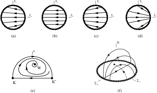
Figure 1: The phase portraits of the stationary Bianchi type II models corresponding to (a) the $N=0$ boundary for $1<\gamma<6/5$, (b) the $N=0$ boundary for $\gamma=6/5$, (c) the $N=0$ boundary for $6/5<\gamma<2$, (d) the vacuum boundary, $\Omega=0$ projected onto the $\Sigma_{\pm}$-plane, (e) the LRS submanifold, $\Sigma_{-}=0$ and (e) the full phase space.

So far we have only discussed the mathematical features of the stationary type II models. However, they might also be of some physical interest. Wainwright has speculated that the solution corresponding to the equilibrium point $W$ might be interpreted as an approximation to the interior of a rotating disc of matter [3]. This interpretation should also pertain to the non-self-similar LRS models and perhaps also to the non-LRS models since they asymptotically approach $W$. However, the main importance of the present models is probably as part of a bigger picture where they may act as building blocks. The phase space of the present models form part of the boundary of more general stationary Bianchi models and hypersurface self-similar models (see [2]). These models in turn form part of the boundary of more general models like the physically interesting $G_{2}$-models, see e.g. [7]. When studying these models one thus have to be observant of the behavior associated with the present heteroclinic cycle which could be expected to describe asymptotic or intermediate oscillating spatial behavior.

Appendix A The non-LRS exact solution

The line element for the non-LRS exact solution is given by

$$ds^{2} = -[x(x+a)]^{1/2}\left(dt+cydz\right)^{2}+[x(x+a)]^{q}dx^{2}$$ (24)

$$\quad+x^{p_{+}}(x+a)^{p_{-}}dy^{2}+x^{p_{-}}(x+a)^{p_{+}}dz^{2}\ ,$$

with

$$q = -\frac{3\gamma-4}{4(\gamma-1)}\ ,\quad p_{\pm}=\frac{3\gamma-2\pm\delta}{8(\gamma-1)}\ ,$$

$$\delta = \sqrt{(11\gamma-10)(3\gamma-2)}\ ,\quad c^{2}=\frac{5\gamma^{2}-4}{16(\gamma-1)^{2}}\ ,$$ (25)

where $a$ is a constant. Setting $a=0$ yields the self-similar solution of [3]. For the remaining non-self-similar solutions one can set $a=1$ by using the scale invariance.

References

[1]
J. Wainwright and G. F. R. Ellis ed., Dynamical systems in
cosmology (Cambridge University Press, Cambridge, 1997)
[2]
U. S. Nilsson and C. Uggla, Hypersurface homogeneous and
hypersurface self-similar models, submitted to
Class. Quant. Grav
[3]
J. Wainwright, Galaxies, Axisymmetric systems and
Relativity, ed. M. A. H. MacCallum (Cambridge University Press, Cambridge,
1985)
[4]
C. Uggla, R. T. Jantzen and K. Rosquist, Phys. Rev. D 51, 5522 (1995)
[5]
C. Uggla, Class. Quantum Grav. 6, 383 (1989)
[6]
J. Wainwright and L. Hsu, Class. Quantum Grav. 6, 1409 (1989)
[7]
C. G. Hewitt and J. Wainwright, Class. Quantum Grav. 7, 2295 (1990)