Lorentzian Approach to Black Hole Thermodynamics in the Hamiltonian Formulation

Abstract

In this work, we extend the analysis of Brown and York to find the quasilocal energy in a spherical box in the Schwarzschild spacetime. Quasilocal energy is the value of the Hamiltonian that generates unit magnitude proper-time translations on the box orthogonal to the spatial hypersurfaces foliating the Schwarzschild spacetime. We call this Hamiltonian the Brown-York Hamiltonian. We find different classes of foliations that correspond to time-evolution by the Brown-York Hamiltonian. We show that although the Brown-York expression for the quasilocal energy is correct, one needs to supplement their derivation with an extra set of boundary conditions on the interior end of the spatial hypersurfaces inside the hole in order to obtain it from an action principle. Replacing this set of boundary conditions with another set yields the Louko-Whiting Hamiltonian, which corresponds to time-evolution of spatial hypersurfaces in a different foliation of the Schwarzschild spacetime. We argue that in the thermodynamical picture, the Brown-York Hamiltonian corresponds to the internal energy whereas the Louko-Whiting Hamiltonian corresponds to the Helmholtz free energy of the system. Unlike what has been the usual route to black hole thermodynamics in the past, this observation immediately allows us to obtain the partition function of such a system without resorting to any kind of Euclideanization of either the Hamiltonian or the action. In the process, we obtain some interesting insights into the geometrical nature of black hole thermodynamics.

I Introduction

After more than two decades of investigations, black hole thermodynamics is still one of the most puzzling subjects in theoretical physics. One approach to studying the thermodynamical aspects of a black hole involves considering the evolution of quantum matter fields propagating on a classical (curved) background spacetime. This gives rise to the phenomenon of black hole radiation that was discovered by Hawking in 1974 [1]. Combining Hawking’s discovery of black hole radiance with the classical laws of black hole mechanics [2], leads to the laws of black hole thermodynamics. The entropy of a black hole obtained from this approach may be interpreted as resulting from averaging over the matter field degrees of freedom lying either inside the black hole [5] or, equivalently, outside the black hole [6], as was first anticipated by Bekenstein [3] even before Hawking’s discovery. The above approach was further developed in the following years [4, 7].

A second route to black hole thermodynamics involves using the path-integral approach to quantum gravity to study vacuum spacetimes (i.e., spacetimes without matter fields). In this method, the thermodynamical partition function is computed from the propagator in the saddle point approximation [8, 9] and it leads to the same laws of black hole thermodynamics as obtained by the first method. The second approach was further developed in the following years [10, 11, 12, 13, 14, 15, 16]. The fact that the laws of black hole thermodynamics can be derived without considering matter fields, suggests that there may be a purely geometrical (spacetime) origin of these laws. However, a complete geometrical understanding of black hole thermodynamics is not yet present.

In general, a basic understanding of the thermodynamical properties of a system requires a specification of the system’s (dynamical) degrees of freedom (d.o.f.). Obtaining such a specification is a nontrivial matter in quantum gravity. In the path-integral approach one avoids the discussion of the dynamical d.o.f.. There, the dominant contribution to the partition function comes from a saddle point, which is a classical Euclidean solution [8]. Calculating the contribution of such a solution to the partition function does not require an identification of what the dynamical d.o.f.’s of this solution are. Though providing us with an elegant way of getting the laws of black hole thermodynamics, the path-integral approach does not give us the basic (dynamical) d.o.f. from which we can have a better geometrical understanding of the origin of black hole thermodynamics.

It was only recently that the dynamical geometric d.o.f. for a spherically symmetric vacuum Schwarzschild black hole were found [17, 18] under certain boundary conditions . In particular, by considering general foliations of the complete Kruskal extension of the Schrawzschild spacetime, Kuchař [18] finds a reduced system of one pair of canonical variables that can be viewed as global geometric d.o.f.. One of these is the Schwarzschild mass, while the other one, its conjugate momentum, is the difference between the parametrization times at right and left spatial infinities. Using the approach of Kuchař, recently Louko and Whiting [19] (henceforth referred to as LW) studied black hole thermodynamics in the Hamiltonian formulation. As shown in Fig. 2, they considered a foliation in which the spatial hypersurfaces are restricted to lie in the right exterior region of the Kruskal diagram and found the corresponding reduced phase space system. This enabled them to find the unconstrained Hamiltonian (which evolves these spatial hypersurfaces) and canonically quantize this reduced theory. They then obtain the Schrödinger time-evolution operator in terms of the reduced Hamiltonian. The partition function $Z$ is defined as the trace of the Euclideanised time-evolution operator $\hat{K}_{\rm E}$, namely, $Z=\mbox{Tr}(\hat{K}_{\rm E})$, where the hat denotes a quantum operator. This partition function has the same expression as the one obtained from the path-integral approach and expectedly yields the laws of black hole thermodynamics.

In a standard thermodynamical system it is not essential to consider Euclidean-time action in order to study the thermodynamics. If $\hat{H}$ is the Lorentzian time-independent Hamiltonian of the system, then the partition function is defined as

$$Z=\mbox{Tr exp}(-\beta\hat{H})\ \ ,$$ (1)

where $\beta$ is the inverse temperature of the system in equilibrium. However, in many cases (especially, in time- independent systems) the Euclidean time-evolution operator turns out to be the same as $\exp(-\beta\hat{H})$. Nevertheless, there are cases where, as we will see in section II B, the Euclidean time-evolution operator is not the same as $\mbox{exp}(-\beta\hat{H})$. This is the case for example in the LW approach, i.e., $(\hat{K}_{\rm E})_{\rm LW}\neq\mbox{exp}(-\beta\hat{\sf h})$, where $\hat{\sf h}$ is the reduced Hamiltonian of the quantized LW system. There is a geometrical reason for this inequality and in this work we discuss it in detail. In this paper, we ask if there exists a Hamiltonian $\hat{H}$ (which is associated with certain foliations of the Schwarzschild spacetime) appropriate for finding the partition function of a Schwarzschild black hole enclosed inside a finite-sized box using (1). Such a procedure will not resort to Euclideanization. In our quest to obtain the Hamiltonian that is appropriate for defining the partition function for (1), we also clarify the physical significance of the LW Hamiltonian. By doing so we hope to achieve a better understanding of the geometrical origin of the thermodynamical aspects of a black hole spacetime.

In a previous work [20], Brown and York (henceforth referred to as BY) found a general expression for the quasilocal energy on a timelike two-surface that bounds a spatial three-surface located in a spacetime region that can be decomposed as a product of a spatial three-surface and a real line interval representing time. From this expression they obtained the quasilocal energy inside a spherical box centered at the origin of a four-dimensional spherically symmetric spacetime. They argued that this expression also gives the correct quasilocal energy on a box in the Schwarzschild spacetime. In this paper we show that, although their expression for the quasilocal energy on a box in the Schwarzschild spacetime is correct, the analysis they use to obtain it requires to be extended when applied to the case of Schwarzschild spacetime. In this case, one needs to impose extra boundary conditions at the timelike boundary inside the hole (see Fig. 3). As mentioned above, in principle, one can use the Hamiltonian $\hat{\sf H}$ so obtained to evaluate the partition function, $Z={\rm Tr}\exp(-\beta\hat{\sf H})$. This partition function corresponds to the canonical ensemble and describes the thermodynamics of a system whose volume and temperature are fixed but whose energy content is permitted to vary. Such a Hamiltonian, $\hat{\sf H}$ would then lead to a description of black hole thermodynamics without any sort of Euclideanisation. The only obstacle to this route to the partition function is that the trace can be evaluated only if one knows the density of the energy eigenstates. Unfortunately, without knowing what the thermodynamical entropy of the system is, it is not clear how to find this density in terms of the reduced phase-space variables of Kuchař [18]. So how can one derive the thermodynamical laws of the Schwarzschild black hole using a Lorentzian Hamiltonian without knowing the density of states?

Based on an observation that identifies the thermodynamical roles of the BY and the LW Hamiltonians we succeed in studying black hole thermodynamics within the Hamiltonian formulation but without Euclideanization. In section II we describe the thermodynamical roles of the BY and the LW Hamiltonians. Identifying these roles allows us to immediately calculate the partition function and recover the thermodynamical properties of the Schwarzschild black hole. In section III we study the geometrical significance of these Hamiltonians. In particular, we extend the work of Brown and York [20] to find the nature of the spatial slices that are evolved by the BY Hamiltonian in the full Kruskal extension of the Schwarzschild spacetime. In section IV we use the observations made in sections II and III to ascribe geometrical basis to the thermodynamical parameters of the system, thus gaining insight into the geometrical nature of black hole thermodynamics.

We conclude the paper in section V by summarising our results and discussing the connection between the foliation geometry and equilibrium black hole thermodynamics. In appendix A we extend our results to the case of two-dimensional dilatonic black holes. In appendix B we discuss an alternative foliation (see Fig. 4), in which the spatial slices are again evolved by the BY Hamiltonian ${\sf H}$. This illustrates the non-uniqueness of the foliation associated with the BY Hamiltonian.

We shall work throughout in “geometrized-units” in which $c=G=1$.

II Thermodynamical Considerations

A The Brown-York Hamiltonian

It was shown by Brown and York [20] that in 4D spherically symmetric Einstein gravity, the quasilocal energy of a system that is enclosed inside a spherical box of finite surface area and which can be embedded in an asymptotically flat space is [20]

$${\sf H}=\left(1-\sqrt{1-{2{\bf m}\over B}}\right)B,$$ (2)

where ${\bf m}$ is the ADM mass of the spacetime and $B$ is the fixed curvature radius of the box with its origin at the center of symmetry. We will call ${\sf H}$ the Brown-York Hamiltonian.

The Brown and York derivation of the quasilocal energy can be summarised as follows. The system they consider is a spatial three-surface $\Sigma$ bounded by a two-surface ${\sf B}$ in a spacetime region that can be decomposed as a product of a spatial three-surface and a real line interval representing time (see Fig. 1). The time evolution of the two-surface boundary ${\sf B}$ is the timelike three-surface boundary ${}^{3}{\sf B}$. They then obtain a surface stress-tensor on the boundary by taking the functional derivative of the action with respect to the three-metric on ${}^{3}{\sf B}$. The energy surface density is the projection of the surface stress tensor normal to a family of spacelike two-surfaces like ${\sf B}$ that foliate ${}^{3}{\sf B}$. The integral of the energy surface density over such a two-surface ${\sf B}$ is the quasilocal energy associated with a spacelike three-surface $\Sigma$ whose orthogonal  intersection with ${}^{3}{\sf B}$ is the two-boundary ${\sf B}$.

As argued by BY, Eq. (2) also describes the total energy content of a box enclosing a Schwarzschild hole. One would thus expect to obtain the corresponding partition function from it by the prescription $Z={\rm Tr}\exp(-\beta\hat{\sf H})$. As mentioned above, the only obstacle to this calculation is the lack of knowledge about the density of states of the system, which is needed to evaluate the trace. However, as we discuss in the next subsection, there is another Hamiltonian associated with the Schwarzschild spacetime that allows us to obtain the relevant partition function without Euclideanization. This is the Louko-Whiting Hamiltonian.

B The Louko-Whiting Hamiltonian

In their quest to obtain the partition function for the Schwarzschild black hole in the Hamiltonian formulation, LW found a Hamiltonian that time-evolves spatial hypersurfaces in a Schwarzschild spacetime of mass ${\bf m}$ such that the hypersurfaces extend from the bifurcation 2-sphere to a timelike box-trajectory placed at a constant curvature radius of $R=B$ (see Fig. 2). As we will show in the next subsection, the LW Hamiltonian describes the correct free energy of a Schwarzschild black hole enclosed inside a box in the thermodynamical picture. The LW Hamiltonian is

$${\bf h}(t)=\left(1-\sqrt{1-{2{\bf m}\over B}}\right)BQ_{B}(t)-2{\bf N}_{0}(t){\bf m}^{2},$$ (3)

where generically $Q_{B}$ and ${\bf N}_{0}$ are functions of time $t$, which labels the spatial hypersurfaces. Physically, $Q_{B}\equiv\sqrt{-g_{tt}}\>$, where $(-g_{tt})$ is the time-time component of the spacetime metric on the box. On the other hand, the physical meaning of ${\bf N}_{0}$ is as follows. On a classical solution, consider the future timelike unit normal $n^{a}(t)$ to a constant $t$ hypersurface at the bifurcation two-sphere (see Fig. 2). Then ${\bf N}_{0}$ is the rate at which the constant $t$ hypersurfaces are boosted at the bifurcation 2-sphere:

$$n^{a}(t_{1})n_{a}(t_{2})=-\cosh\left(\int_{t_{1}}^{t_{2}}{\bf N}_{0}\>dt\right)\ \ ,$$ (4)

where $t=t_{1}$ is the initial hypersurface and $t=t_{2}$ is the boosted hypersurface.

If one is restricted to a foliation in which the spatial hypersurfaces approach the box along surfaces of constant proper time on the box, then $Q_{B}=1$. On classical solutions, the spatial hypersurfaces approach the bifurcation 2-sphere along constant Killing-time hypersurfaces (see the paragraph containing Eqs. (III B 1) in section III B). The LW fall-off conditions (III B 1), which are imposed on the ADM variables at the bifurcation 2-sphere, can be used to show that on solutions, ${\bf N}_{0}=\kappa\>dT/dt$, where $T$ is the Killing time and $\kappa=(4{\bf m})^{-1}$ is the surface gravity of a Schwarzschild black hole. In the particular case where the label time $t$ is taken to be the proper time on the box, we have

$${\bf N}_{0}=\left[4{\bf m}\sqrt{1-{2{\bf m}\over B}}\>\right]^{-1}\ \ .$$ (5)

With such an identification of the label time $t$, Eq. (3) shows that on classical solutions the time-evolution of these spatial hypersurfaces is given by the Hamiltonian

$${\sf h}=\left(1-\sqrt{1-{2{\bf m}\over B}}\right)B-2{\bf N}_{0}{\bf m}^{2},$$ (6)

where ${\bf N}_{0}$ is given by (5).

One may now ask if one can use the LW Hamiltonian (6) to obtain a partition function for the system and study its thermodynamical properties. Unfortunately, one cannot do so in a straightforward manner. First, one cannot replace $\hat{H}$ in (1) by $\hat{\sf h}$, the quantum counterpart of (6), to obtain the partition function. The reason is that classically ${\sf h}$ does not give the correct energy of the system; the BY Hamiltonian ${\sf H}$ of (2) does. To avoid this problem, LW first construct the Schrödinger time-evolution operator $\hat{K}\equiv\exp(-i\int\hat{\sf h}dt)$. They then Euclideanize this operator and use it to obtain the partition function $Z={\rm Tr}({\hat{K}}_{\rm E})$. The partition function so obtained does not equal ${\rm Tr}\exp(-\beta\hat{\sf h})$, but rather it turns out to be the same as that obtained via the path integral approach of Gibbons and Hawking [8]. However, apart from this end result, a justification at some fundamental level has been lacking as to why the LW Hamiltonian (6) and not any other Hamiltonian (eg., (2)) should be used to obtain the partition function using the LW procedure.

In the next subsection, we will find the thermodynamical roles played by the BY and LW Hamiltonians. We will also show how this helps us in obtaining the partition function without Euclideanization. This way we will avoid the ambiguity mentioned above that arises in the LW-method of constructing the partition function.

C Internal Energy and Free Energy

As argued by Brown and York [20], on solutions, the BY Hamiltonian ${\sf H}$ in Eq. (2) denotes the internal energy ${\cal E}$ residing within the box:

$${\cal E}=\left(1-\sqrt{1-{2{\bf m}\over B}}\right)B.$$ (7)

In fact Eq. (7) can be shown to yield the first law of black hole thermodynamics

$$\Delta{\cal E}=-s\>\Delta(4\pi B^{2})+\left(8\pi{\bf m}\sqrt{1-{2{\bf m}\over B}}\right)^{-1}\Delta(4\pi{\bf m}^{2}),$$ (8)

where $s$ is the surface pressure on the box-wall [20]

$$s\equiv{1\over 8\pi B}\left({1-{\bf m}/B\over\sqrt{1-2{\bf m}/B}}-1\right).$$ (9)

The first term on the rhs of (8) is negative of the amount of work done by the system on its surroundings and, with hindsight, the second term is the product ${\cal T}\Delta{\cal S}$, where ${\cal T}$ is the temperature and ${\cal S}$ is the entropy of the system. We will not assume the latter in the following analysis; rather we will deduce the form of ${\cal T}$ and ${\cal S}$ from first principles.

We next show that the LW Hamiltonian ${\sf h}$ of Eq. (6) plays the role of Helmholtz free energy of the system. Recall that the Helmholtz free energy ${\cal F}$ is defined as

$${\cal F}=\>{\cal E}\>-\>{\cal T}{\cal S},$$ (10)

where ${\cal E}$ is the internal energy. Thus in an isothermal and reversible process, the first law of thermodynamics implies that the amount of mechanical work done by a system, $W$, is equal to the decrease in its free energy, i.e.,

$$W=-\Delta{\cal F}\ \ .$$ (11)

As a corollary to this statement it follows that for a mechanically isolated system at a constant temperature, the state of equilibrium is the state of minimum free energy.

We now show that under certain conditions on the foliation of the spacetime with spatial hypersurfaces, the LW Hamiltonian ${\sf h}$ in Eq. (6) plays the role of free energy. We choose a foliation such that on solutions the lapse ${\bf N}_{0}$ obeys (5). Using the expression (7) for ${\cal E}$, the Hamiltonian ${\sf h}$ in Eq. (6) can be rewritten as

$${\sf h}={\cal E}-2{\bf N}_{0}{\bf m}^{2}\ \ .$$ (12)

Now let us perturb ${\sf h}$ about a solution by perturbing ${\bf m}$ and $B$ such that ${\bf N}_{0}$ itself is held fixed. Then

$$\Delta{\sf h}=\Delta{\cal E}-{{\bf N}_{0}\over 2\pi}\Delta(4\pi{\bf m}^{2})\ \ .$$ (13)

Note that keeping ${\bf N}_{0}$ fixed, i.e., $\Delta{\bf N}_{0}=0$, does not necessarily imply through (5) that $\Delta{\bf m}$ and $\Delta B$ are not independent perturbations. This is because, in general, the perturbed ${\sf h}$ may not correspond to a solution and hence the perturbed ${\bf N}_{0}$ need not have the form (5). However, here we will assume that the perturbations do not take us off the space of static solutions and, therefore, the perturbed ${\bf N}_{0}$ has the form (5). Hence in our case $\Delta{\bf m}$ and $\Delta B$ are not independent perturbations. Using (8) and (5) in (13) yields

$$\Delta{\sf h}=-s\Delta(4\pi B^{2})=-W\ \ .$$ (14)

Finally, from (14) and (11) we get

$${\sf h}={\cal F}+c\ \ ,$$ (15)

where $c$ is a constant independent of ${\bf m}$. To find $c$, we take the limit ${\bf m}\to 0$. In this limit both ${\sf h}$ and ${\cal F}$ vanish and, therefore, $c$ has to be zero.

Another way to see that $c$ should vanish is to identify the geometric quantity ${\bf N}_{0}$ with the temperature, ${\cal T}$, of the system (up to a multiplicative constant). Then the perturbation (13) in ${\sf h}$, keeping ${\bf N}_{0}$ (and, therefore, ${\cal T}$) fixed, describes an isothermal process. But Eq. (15) shows that $c$ has to be an extensive function of thermodynamic invariants of the isothermal process since ${\sf h}$ and ${\cal F}$ are both extensive. The only thermodynamic quantity that we assume to be invariant in this isothermal process is the temperature ${\cal T}$. But since ${\cal T}$ is not extensive, $c$ has to be zero. The fact that ${\bf N}_{0}$ indeed determines the temperature of the system will be discussed in detail in a later section.

The above proof of the LW Hamiltonian being the Helmholtz free energy immediately allows us to calculate the partition function for a canonical ensemble of such systems,

$$Z=\exp\left(-\beta{\cal F}\right)\ \ ,$$ (16)

by simply putting ${\cal F}={\sf h}$. In this way we recover the thermodynamical properties of a Schwarzschild black hole without Euclideanization. We will do so in detail in section IV but first we establish the geometrical significance of BY and LW Hamiltonians in the next section.

III Geometrical considerations: Dynamics

A study of the geometrical roles of the BY and LW Hamiltonians provides the geometrical basis for the thermodynamical parameters associated with a black hole that were discussed in the preceeding section. In this section we begin by setting up the Hamiltonian formulation appropriate for the two sets of boundary conditions that lead to the BY and LW Hamiltonians as being the unconstrained Hamiltonians that generate time-evolution of foliations in Schwarzschild spacetime. The notation follows that of Kuchař [18] and LW.

A general spherically symmetric spacetime metric on the manifold ${\bf R}\times{\bf R}\times S^{2}$ can be written in the ADM form as

$$ds^{2}=-N^{2}dt^{2}+\Lambda^{2}{(dr+N^{r}dt)}^{2}+R^{2}d\Omega^{2}\ \ ,$$ (17)

where $N$, $N^{r}$, $\Lambda$ and $R$ are functions of $t$ and $r$ only, and $d\Omega^{2}$ is the metric on the unit two-sphere. We will choose our boundary conditions in such a way that the radial proper distance $\int\Lambda\,dr$ on the constant $t$ surfaces is finite. This implies that the radial coordinate $r$ have a finite range, which we take to be $[0,1]$, without any loss of generality. The spatial metric and the spacetime metric will be assumed to be nondegenerate, in particular, $\Lambda$, $R$, and $N$ are taken to be positive.

For the metric (17), the Einstein-Hilbert action is

$$S_{\Sigma}[R,\Lambda;N,N^{r}]$$ (18)

$$=\int dt\int_{0}^{1}dr\,\bigg{[} -N^{-1}\left(R\bigl{(}-{\dot{\Lambda}}+(\Lambda N^{r})^{\prime}\bigr{)}(-{\dot{R}}+R^{\prime}N^{r})+\frac{1}{2}\Lambda{(-{\dot{R}}+R^{\prime}N^{r})}^{2}\right)$$ (20)

$$+N\left(-\Lambda^{-1}RR^{\prime\prime}+\Lambda^{-2}RR^{\prime}\Lambda^{\prime}-\frac{1}{2}\Lambda^{-1}{R^{\prime}}^{2}+\frac{1}{2}\Lambda\right)\bigg{]}\ \ ,$$

where the subscript $\Sigma$ denotes that $S_{\Sigma}$ is a hypersurface action that is defined only up to the possible addition of boundary terms. Above, the overdot and the prime denote $\frac{\partial}{\partial t}$  and  $\frac{\partial}{\partial r}$, respectively. The equations of motion derived from (20) are the full Einstein equations for the metric (17), and they imply that every classical solution is part of a maximally extended Schwarzschild spacetime, where the value of the Schwarzschild mass $M$ may be positive, negative, or zero. In what follows, we will choose our boundary conditions such that $M>0$. We shall discuss the boundary conditions and the boundary terms after passing to the Hamiltonian formulation.

The momenta conjugate to $\Lambda$ and $R$ are found from the Lagrangian action (20) to be

$$P_{\Lambda} = -N^{-1}R\left({\dot{R}}-R^{\prime}N^{r}\right)\ \ ,$$ (22)

$$P_{R} = -N^{-1}\left(\Lambda({\dot{R}}-R^{\prime}N^{r})+R\bigl{(}{\dot{\Lambda}}-(\Lambda N^{r})^{\prime}\bigr{)}\right)\ \ .$$ (23)

A dual-Legendre transformation then yields the Hamiltonian action

$$S_{\Sigma}[\Lambda,R,P_{\Lambda},P_{R};N,N^{r}]=\int dt\int_{0}^{1}dr\left(P_{\Lambda}{\dot{\Lambda}}+P_{R}{\dot{R}}-NH-N^{r}H_{r}\right)\ \ ,$$ (24)

where the super-Hamiltonian $H$ and the radial supermomentum $H_{r}$ are

$$H = -R^{-1}P_{R}P_{\Lambda}+\frac{1}{2}R^{-2}\Lambda P_{\Lambda}^{2}+\Lambda^{-1}RR^{\prime\prime}-\Lambda^{-2}RR^{\prime}\Lambda^{\prime}+\frac{1}{2}\Lambda^{-1}{R^{\prime}}^{2}-\frac{1}{2}\Lambda\ \ ,$$ (26)

$$H_{r} = P_{R}R^{\prime}-\Lambda P_{\Lambda}^{\prime}\ \ .$$ (27)

It can be verified that the Poisson brackets of the constraints close according to the radial version of the Dirac algebra [21].

We next consider the boundary terms that must be added to the hypersurface action (24) for the total action to yield, upon variation, only a volume term corresponding to the equations of motion. However, the boundary terms depend intricately on the choice of the spacetime foliation. Different foliations require different boundary conditions on the geometric variables in the variational analysis, thus requiring the addition of different boundary terms to (24). As is well known in general relativity, it is these boundary terms that determine the true Hamiltonian of the system. Hence, as we show below explicitly, this implies that different foliations correspond to different Hamiltonians, which are the generators of time-evolution of the spatial slices in the foliations.

A The Brown-York Hamiltonian

In general, the analysis of Brown and York (see subsection II A) breaks down in cases where spacetime regions of non-trivial topologies are enclosed inside the spherical box, particularly so in the case of a Schwarzschild black hole enclosed inside the box. As we show below, in this case one is forced to introduce an “inner”-boundary where the spatial hypersurfaces of Brown and York must extend to. This fact becomes transparent when one looks at the full Kruskal extension of the Schwarzschild metric. There, one begins by performing a $(3+1)$ decomposition of the spacetime in terms of a one-parameter family of spatial hypersurfaces. The Kruskal diagram (see Figs. 2 and 3) shows that any such foliation would necessarily require two boundaries: an outer boundary and an inner boundary. The Hamiltonian that evolves these spatial hypersurfaces in time will in general depend on the boundary conditions specified on these 2-boundaries. In this section we show that the spatial hypersurfaces that are evolved by the Hamiltonian corresponding to the quasilocal energy, given in (2), are ones that extend from the box (the outer timelike boundary), on the right end, to an inner timelike boundary located completely inside the dynamical region of the Kruskal diagram, on the left end.

1 Boundary conditions

We first find the boundary conditions and the foliation that correspond to time evolution by the BY Hamiltonian and later we compare these with those corresponding to the LW Hamiltonian. At $r=0$, we prescribe the following fall-off conditions

$$\Lambda(t,r) = \Lambda_{0}(t)+O(r^{2})\ \ ,$$ (29)

$$R(t,r) = R_{0}(t)+R_{2}(t)r^{2}+O(r^{4})\ \ ,$$ (30)

$$P_{\Lambda}(t,r) = P_{\Lambda 0}(t)+O(r^{2})\ \ ,$$ (31)

$$P_{R}(t,r) = P_{R0}(t)+O(r^{2})\ \ ,$$ (32)

$$N(t,r) = N_{0}(t)+O(r^{2})\ \ ,$$ (33)

$$N^{r}(t,r) = N^{r}_{1}(t)r+O(r^{3})\ \ ,$$ (34)

where $\Lambda_{0}$ and $R_{0}$ are positive. This ensures that on classical solutions $M$ is positive. Also $N_{1}\geq 0$. Here $O(r^{n})$ stands for a term whose magnitude at $r\to 0$ is bounded by $r^{n}$ times a constant, and whose $k$’th derivative at $r\to 0$ is similarly bounded by $r^{n-k}$ times a constant for $1\leq k\leq n$. The fact that the shift $N^{r}(t,r)$ vanishes as $r\to 0$ implies that on solutions, the inner timelike boundary lies along a constant Killing-time surface located completely in the past and the future dynamical regions and cutting across the bifurcation two-sphere. Also, on solutions, the variable $R_{0}$ corresponds to the throat-radius.

It is straightforward to verify that the conditions (III A 1) are consistent with the equations of motion: Provided that the constraints obey $H=0=H^{r}$ and the fall-off conditions (29)–(32) hold for the initial data, and provided that the lapse and shift satisfy (33) and (34), it then follows that the fall-off conditions (29)–(32) are preserved in time by the time-evolution equations.

On the other hand, at $r=1$, the boundary conditions are as follows: We fix $R$ and $-g_{tt}=N^{2}-{(\Lambda N^{r})}^{2}$ to be prescribed positive-valued functions of $t$. This means fixing the metric on the three-surface $r=1$ to be timelike. In the classical solutions, the surface $r=1$ is located in the right exterior region of the Kruskal extension of the Schwarzschild spacetime.

We now give an action principle appropriate for these boundary conditions. To begin, note that the surface action $S_{\Sigma}[\Lambda,R,P_{\Lambda},P_{R};N,N^{r}]$ in (24) is well defined under the above conditions. Consider the total action

$$S[\Lambda,R,P_{\Lambda},P_{R};N,N^{r}]=S_{\Sigma}[\Lambda,R,P_{\Lambda},P_{R};N,N^{r}]+S_{\partial\Sigma}[\Lambda,R,P_{\Lambda},P_{R};N,N^{r}]\ \ ,$$ (35)

where the boundary action is given by

$$S_{\partial\Sigma}[\Lambda,R,P_{\Lambda},P_{R};N,N^{r}]$$ (36)

$$=\int dt{\Biggl{[}NRR^{\prime}\Lambda^{-1}-N^{r}\Lambda P_{\Lambda}-\frac{1}{2}R{\dot{R}}\ln\left|{N+\Lambda N^{r}\over N-\Lambda N^{r}}\right|\Biggr{]}}_{r=1}\ \ ,$$ (37)

where $\left[{\it term}\right]_{a}$ is value of the term evaluated at $r=a$. The variation of the total action (35) can be written as a sum of a volume term proportional to the equations of motion, boundary terms from the initial and final spatial surfaces, and boundary terms from $r=0$ and $r=1$. The boundary terms from the initial and final spatial surfaces take the usual form

$$\pm\int_{0}^{1}dr\,(P_{\Lambda}\delta\Lambda+P_{R}\delta R)\ \ ,$$ (38)

with the upper (lower) sign corresponding to the final (initial) surface. These terms vanish provided we fix the initial and final three-metrics. The boundary term from $r=0$ vanishes under the fall-off conditions specified in (III A 1). As will be shown in subsection III A 3, this is crucial in obtaining a reduced Hamiltonian that corresponds to the correct quasilocal energy. The boundary term from $r=1$ reads

$$\int dt\Bigg{[} \left(-P_{R}N^{r}+\Lambda^{-1}{(NR)}^{\prime}\right)\delta R-\frac{1}{2}\ln\left|{N+\Lambda N^{r}\over N-\Lambda N^{r}}\right|\,\delta(R{\dot{R}})$$ (41)

$$+\frac{1}{2}N^{-1}R\left(\Lambda N^{r}{\dot{R}}{\left(N^{2}-{(\Lambda N^{r})}^{2}\right)}^{-1}+\Lambda^{-1}R^{\prime}\right)\delta\!\left(N^{2}-{(\Lambda N^{r})}^{2}\right)$$

$${-\left(P_{\Lambda}+N^{-1}R({\dot{R}}-R^{\prime}N^{r})\right)\delta(\Lambda N^{r})\Bigg{]}}_{r=1}\ \ .$$

Since $R$ and $N^{2}-{(\Lambda N^{r})}^{2}$ are fixed at $r=1$, the first three terms in (41) vanish. The integrand in the last term in (41) is proportional to the equation of motion (22), which is classically enforced for $0<r<1$ by the volume term in the variation of the action. Therefore, for classical solutions, also the last term in (41) will vanish by continuity.

Thus the action (35) is appropriate for a variational principle which fixes the initial and final three-metrics, and the three-metric on the timelike boundary at $r=1$. Each classical solution belongs to that region of a Kruskal diagram that lies within two timelike boundaries such that the inner boundary lies along a constant Killing-time surface located completely in the dynamical regions and the outer boundary is a timelike surface located in the right exterior region (see Fig. 3). The constant $t$ slices are spacelike everywhere between the two timelike boundaries.

2 Canonical transformation

To obtain the reduced action and extract the unconstrained Hamiltonian system one needs to first solve the constraints (26) and (27). In the following, we will follow Kuchař’s way of handling the constraints [18]. It was shown by Kuchař that in the context of a vacuum Schwarzschild spacetime (in the absence of timelike boundaries) there exists a set of new variables, which are related to the ADM variables through a canonical transformation, such that in terms of the new variables the constraints are remarkably simple and solvable. This allows one to perform a Hamiltonian reduction. In this section we show that the canonical transformation given by Kuchař from the ADM variables $\left\{\Lambda,P_{\Lambda};R,P_{R}\right\}$ to the new variables $\left\{M,P_{M};{\sf R},P_{\sf R}\right\}$ is readily adapted to our boundary conditions. As mentioned earlier, the boundary conditions ensure that $M>0$.

Recall from [18] that the new variables $\left\{M,P_{M};{\sf R},P_{\sf R}\right\}$ are defined by

$$M =\frac{1}{2}R(1-F)\ \ ,$$ (43)

$$P_{M} =R^{-1}F^{-1}\Lambda P_{\Lambda}\ \ ,$$ (44)

$${\sf R} =R\ \ ,$$ (45)

$$P_{\sf R} =P_{R}-\frac{1}{2}R^{-1}\Lambda P_{\Lambda}-\frac{1}{2}R^{-1}F^{-1}\Lambda P_{\Lambda}$$ (47)

$$\;-R^{-1}\Lambda^{-2}F^{-1}\left({(\Lambda P_{\Lambda})}^{\prime}(RR^{\prime})-(\Lambda P_{\Lambda}){(RR^{\prime})}^{\prime}\right)\ \ ,$$

where

$$F={\left({R^{\prime}\over\Lambda}\right)}^{2}-{\left({P_{\Lambda}\over R}\right)}^{2}\ \ .$$ (48)

In the classical solution, $M$ is the value of the Schwarzschild mass and $-P_{M}$ is the derivative of the Killing time with respect to $r$. A pair of quantities which will become new Lagrange multipliers are defined by

$${\sf N} = {(4M)}^{-1}\left(NF^{-1}\Lambda^{-1}R^{\prime}-N^{r}R^{-1}F^{-1}\Lambda P_{\Lambda}\right)\ \ ,$$ (50)

$$N^{\sf R} = N^{r}R^{\prime}-NR^{-1}P_{\Lambda}\ \ .$$ (51)

Using arguments similar to Kuchař and LW, it can be shown that under our boundary conditions the transformation (III A 2) is a canonical transformation, which is also invertible [18].

The Hamiltonian action (24) can now be written in terms of the new variables. Using Eqs. (48), one sees that the constraint terms $NH+N^{r}H_{r}$ in the old surface action (24) take the form $-4{\sf N}MM^{\prime}+N^{\sf R}P_{\sf R}$. Thus the new surface action is

$$S_{\Sigma}[M,{\sf R},P_{M},P_{\sf R};{\sf N},N^{\sf R}]=\int dt\int_{0}^{1}dr\left(P_{M}{\dot{M}}+P_{\sf R}\dot{\sf R}+4{\sf N}MM^{\prime}-N^{\sf R}P_{\sf R}\right)\ \ ,$$ (52)

where the quantities to be varied independently are $M$, ${\sf R}$, $P_{M}$, $P_{\sf R}$, ${\sf N}$, and $N^{\sf R}$. The complete set of equations of motion is

$${\dot{M}} = 0\ \ ,$$ (54)

$${\dot{\sf R}} = N^{\sf R}\ \ ,$$ (55)

$${\dot{P}}_{M} = -4M{\sf N}^{\prime}\ \ ,$$ (56)

$${\dot{P}}_{\sf R} = 0\ \ ,$$ (57)

$$MM^{\prime} = 0\ \ ,$$ (58)

$$P_{\sf R} = 0\ \ .$$ (59)

We now turn to the boundary conditions and boundary terms. As a preparation for this, let us denote by $Q^{2}$ the quantity $-g_{tt}$ when expressed as a function of the new canonical variables and Lagrange multipliers. A short calculation using (III A 2)–(48) yields

$$Q^{2}=-g_{tt}=16M^{2}{\sf F}{\sf N}^{2}-{\sf F}^{-1}{\left(N^{\sf R}\right)}^{2}\ \ .$$ (60)

In general, $Q^{2}$ need not be positive for all values of $r$, even for classical solutions. However, as in subsection III A 1, we shall introduce boundary conditions that fix the intrinsic metric on the three-surface $r=1$ to be timelike, and under such boundary conditions $Q^{2}$ is positive at $r=1$.

Consider now the total action

$$S[M,{\sf R},P_{M},P_{\sf R};{\sf N},N^{\sf R}]=S_{\Sigma}[M,{\sf R},P_{M},P_{\sf R};{\sf N},N^{\sf R}]+S_{\partial\Sigma}[M,{\sf R},P_{M},P_{\sf R};{\sf N},N^{\sf R}]\ \ ,$$ (61)

where the boundary action is given by

$$S_{\partial\Sigma}[M,{\sf R},P_{M},P_{\sf R};{\sf N},N^{\sf R}]$$ (62)

$$= \int dt{\left[{\sf R}\sqrt{{\sf F}Q^{2}+{\dot{\sf R}}^{2}}+\frac{1}{2}{\sf R}\dot{\sf R}\ln\left({\sqrt{{\sf F}Q^{2}+{\dot{\sf R}}^{2}}-\dot{\sf R}\over\sqrt{{\sf F}Q^{2}+{\dot{\sf R}}^{2}}+\dot{\sf R}}\right)\vphantom{{\left|{\sqrt{{\sf F}Q^{2}+{\dot{\sf R}}^{2}}-\dot{\sf R}\over\sqrt{{\sf F}Q^{2}+{\dot{\sf R}}^{2}}+\dot{\sf R}}\right|}^{Q}_{Q}}\right]}_{r=1}$$ (63)

with ${\sf F}=1-2M{\sf R}^{-1}$. Note that the argument of the logarithm in (63) is always positive. The variation of (61) contains a volume term proportional to the equations of motion, as well as several boundary terms. From the initial and final spatial surfaces one gets the usual boundary terms

$$\pm\int_{0}^{1}dr\left(P_{M}\delta M+P_{\sf R}\delta{\sf R}\right)\ \ ,$$ (64)

which vanish provided we fix $M$ and ${\sf R}$ on these surfaces. Similarly one can show that with our choice of boundary conditions (given in section III A 1) the remaining boundary terms from the timelike surfaces at $r=0$ and $r=1$ also vanish.

3 Hamiltonian reduction: the Brown-York Hamiltonian

We now concentrate on the variational principle associated with the action $S[M,{\sf R},P_{M},P_{\sf R};{\sf N},N^{\sf R}]$ (61). We shall reduce the action to the true dynamical degrees of freedom by solving the constraints.

The constraint $MM^{\prime}=0$ (58) implies that $M$ is independent of $r$. We can therefore write

$$M(t,r)={\bf m}(t)\ \ .$$ (65)

Substituting this and the constraint $P_{\sf R}=0$ (59) back into (61) yields the true Hamiltonian action

$$S[{\bf m},{\bf p};{\sf N_{0}};{\sf R}_{\rm B},Q_{\rm B}]=\int dt\left({\bf p}{\dot{\bf m}}-{\bf H}\right)\ \ ,$$ (66)

where

$${\bf p}=\int_{0}^{1}dr\,P_{M}\ \ .$$ (67)

The reduced Hamiltonian ${\bf H}$ in (66) takes the form

$${\bf H}=-{\sf R}_{\rm B}\sqrt{{\sf F}_{\rm B}Q_{\rm B}^{2}+{\dot{\sf R}}_{\rm B}^{2}}-\frac{1}{2}{\sf R}_{\rm B}{\dot{\sf R}}_{\rm B}\ln\left({\sqrt{{\sf F}_{\rm B}Q_{\rm B}^{2}+{\dot{\sf R}}_{\rm B}^{2}}-{\dot{\sf R}}_{\rm B}\over\sqrt{{\sf F}_{\rm B}Q_{\rm B}^{2}+{\dot{\sf R}}_{\rm B}^{2}}+{\dot{\sf R}}_{\rm B}}\right)\ \ .$$ (68)

Here ${\sf R}_{\rm B}$ and $Q_{\rm B}^{2}$ are the values of ${\sf R}$ and $Q^{2}$ at the timelike boundary $r=1$, and ${\sf F}=1-2{\bf m}{\sf R}^{-1}$. As mentioned before, ${\sf R}_{\rm B}$ and $Q_{\rm B}^{2}$ are prescribed functions of time, satisfying ${\sf R}_{\rm B}>0$ and $Q_{\rm B}^{2}>0$. Note that ${\bf H}$ is, in general, explicitly time-dependent.

The variational principle associated with the reduced action (66) fixes the initial and final values of ${\bf m}$. The equations of motion are

$${\dot{\bf m}} = 0\ \ ,$$ (70)

$${\dot{\bf p}} = -{\partial{\bf H}\over\partial{\bf m}}$$ (71)

$$= -{\sf F}_{\rm B}^{-1}\sqrt{{\sf F}_{\rm B}Q_{\rm B}^{2}+{\dot{\sf R}}_{\rm B}^{2}}\ \ .$$ (72)

Equation (70) is readily understood in terms of the statement that ${\bf m}$ is classically equal to the time-independent value of the Schwarzschild mass. To interpret equation (72), recall from Sec. III A 2 that $-P_{M}$ equals classically the derivative of the Killing time with respect to $r$, and ${\bf p}$ therefore equals by (67) the difference of the Killing times at the left and right ends of the constant $t$ surface. As the constant $t$ surface evolves in the Schwarzschild spacetime, (72) gives the negative of the evolution rate of the Killing time at the right end of the spatial surface where it terminates at the outer timelike boundary at $r=1$. Note that ${\dot{\bf p}}$ gets no contribution from the inner timelike boundary located at $r=0$ in the dynamical region. This is a consequence of the fall-off conditions (III A 1) which ensure that on solutions, the rate of evolution of the Killing time at $r=0$ is zero.

The case of interest is when the radius of the ‘outer’ boundary two-sphere does not change in time, i.e., ${\dot{\sf R}}_{\rm B}=0$. In that case the second term in ${\bf H}_{\rm B}$ (68) vanishes, and ${\dot{\bf p}}$ in (72) is readily understood in terms of the Killing time of a static Schwarzschild observer, expressed as a function of the proper time $\int^{t}dt^{\prime}\sqrt{Q_{\rm B}^{2}(t^{\prime})}$ and the blueshift factor ${\sf F}_{\rm B}^{-1/2}$. The reduced Hamiltonian is given by

$${\bf H}=-B\sqrt{{\sf F}_{\rm B}Q_{\rm B}^{2}},$$ (73)

where $B$ is the time-independent value of ${\sf R}_{\rm B}$. Unfortunately, the above Hamiltonian does not vanish as ${\bf m}$ goes to zero. The situation is remedied by adding the $K_{0}=BQ_{\rm B}$ term of Gibbons and Hawking [8] to ${\bf H}$. Physically, this added term arises from the extrinsic curvature of the ‘outer’ boundary two-sphere when embedded in flat spacetime. With the added term, the Hamiltonian becomes

$${\bf H}=\left(1-\sqrt{1-2{\bf m}B^{-1}}\right)BQ_{\rm B}.$$ (74)

This is the quasilocal energy of Brown and York when $Q_{B}=1$. The choice of $Q_{B}$ determines the choice of time in the above Hamiltonian. Setting $Q_{B}=\sqrt{-g_{tt}}=1$ geometrically means choosing a spacetime foliation in which the rate of evolution of the spatial hypersurface on the box is the same as that of the proper time. Then the new Hamiltonian is

$${\sf H}=\left(1-\sqrt{1-2{\bf m}B^{-1}}\right)B\ \ ,$$ (75)

namely, the quasilocal energy (2) in Schwarzschild spacetime. In the next section, we discuss the geometric relevance of the LW Hamiltonian that, as we showed earlier, yields the correct free energy of the system.

B The Louko-Whiting Hamiltonian

We now summarize the LW choice of the foliation of the Schwarzschild spacetime, state the corresponding boundary conditions they imposed, and briefly mention how they obtain their reduced Hamiltonian. The main purpose of this section is to facilitate a comparison between the LW boundary conditions and our choice of the boundary conditions (as discussed in the preceeding subsections) that yield the BY Hamiltonian.

1 Louko-Whiting boundary conditions

As shown in Fig. 2, LW considered a foliation in which the spatial hypersurfaces are restricted to lie in the right exterior region of the Kruskal diagram. Each spatial hypersurface in this region extends from the box at the right end up to the bifurcation 2-sphere on the left end.

The boundary conditions imposed by LW are as follows. At $r\to 0$, they adopt the fall-off conditions

$$\Lambda(t,r) = \Lambda_{0}(t)+O(r^{2})\ \ ,$$ (77)

$$R(t,r) = R_{0}(t)+R_{2}(t)r^{2}+O(r^{4})\ \ ,$$ (78)

$$P_{\Lambda}(t,r) = O(r^{3})\ \ ,$$ (79)

$$P_{R}(t,r) = O(r)\ \ ,$$ (80)

$$N(t,r) = N_{1}(t)r+O(r^{3})\ \ ,$$ (81)

$$N^{r}(t,r) = N^{r}_{1}(t)r+O(r^{3})\ \ ,$$ (82)

where $\Lambda_{0}$ and $R_{0}$ are positive, and $N_{1}\geq 0$. Equations (77) and (78) imply that the classical solutions have a positive value of the Schwarzschild mass, and that the constant $t$ slices at $r\to 0$ are asymptotic to surfaces of constant Killing time in the right hand side exterior region in the Kruskal diagram, all approaching the bifurcation two-sphere as $r\to 0$. The spacetime metric has thus a coordinate singularity at $r\to 0$, but this singularity is quite precisely controlled. In particular, on a classical solution the future unit normal to a constant $t$ surface defines at $r\to 0$ a future timelike unit vector $n^{a}(t)$ at the bifurcation two-sphere of the Schwarzschild spacetime, and the evolution of the constant $t$ surfaces boosts this vector at the rate given by

$$n^{a}(t_{1})n_{a}(t_{2})=-\cosh\left(\int_{t_{1}}^{t_{2}}\Lambda_{0}^{-1}(t)N_{1}(t)\,dt\right)\ \ .$$ (83)

At $r=1$, we fix $R$ and $-g_{tt}=N^{2}-{(\Lambda N^{r})}^{2}$ to be prescribed positive-valued functions of $t$. This means fixing the metric on the three-surface $r=1$, and in particular fixing this metric to be timelike. In the classical solutions, the surface $r=1$ is located in the right hand side exterior region of the Kruskal diagram.

To obtain an action principle appropriate for these boundary conditions, consider the total action

$$S[\Lambda,R,P_{\Lambda},P_{R};N,N^{r}]=S_{\Sigma}[\Lambda,R,P_{\Lambda},P_{R};N,N^{r}]+S_{\partial\Sigma}[\Lambda,R,P_{\Lambda},P_{R};N,N^{r}]\ \ ,$$ (84)

where the boundary action is given by

$$S_{\partial\Sigma}[\Lambda,R,P_{\Lambda},P_{R};N,N^{r}]$$ (85)

$$=\frac{1}{2}\int dt\,{\left[R^{2}N^{\prime}\Lambda^{-1}\right]}_{r=0}\;\;+\int dt{\Biggl{[}NRR^{\prime}\Lambda^{-1}-N^{r}\Lambda P_{\Lambda}-\frac{1}{2}R{\dot{R}}\ln\left|{N+\Lambda N^{r}\over N-\Lambda N^{r}}\right|\Biggr{]}}_{r=1}\ \ .$$ (86)

The variation of the total action (84) can be written as a sum of a volume term proportional to the equations of motion, boundary terms from the initial and final spatial surfaces, and boundary terms from $r=0$ and $r=1$.

To make the action (84) appropriate for a variational principle, one fixes the initial and final three-metrics, the box-radius $R$, and the three-metric on the timelike boundary at $r=1$. These are similar to the boundary conditions that we imposed to obtain the BY Hamiltonian. However, for the LW boundary conditions, one has to also fix the quantity ${\bf N}_{0}\equiv N_{1}\Lambda_{0}^{-1}=\lim_{r\to 0}N^{\prime}\Lambda^{-1}$ at the bifurcation 2-sphere. Each classical solution is part of the right hand exterior region of a Kruskal diagram, with the constant $t$ slices approaching the bifurcation two-sphere as $r\to 0$, and $N_{1}\Lambda_{0}^{-1}$ giving via (83) the rate of change of the unit normal to the constant $t$ surfaces at the bifurcation two-sphere.

Although we are here using geometrized units, the argument of the $\cosh$ in (83) is a truly dimensionless “boost parameter” even in physical units.

2 Hamiltonian reduction: the Louko-Whiting Hamiltonian

To obtain the (reduced) LW Hamiltonian, one needs to solve the super-Hamiltonian and the supermomentum constraints. Just as in the case of the BY Hamiltonian (see subsection III A 2), it helps to first make a canonical transformation to the Kuchař variables (see LW for details). After solving the constraints, one obtains the following reduced action

$$S[{\bf m},{\bf p};{\bf N_{0}};{\sf R}_{\rm B},Q_{\rm B}]=\int dt\left({\bf p}{\dot{\bf m}}-{\bf h}\right)\ \ ,$$ (87)

where

$${\bf p} = \int_{0}^{1}dr\>P_{M}\ \ ,$$ (88)

$${\bf m}(t)=M(t,r)\ \ ,$$ (89)

and the reduced Hamiltonian ${\bf h}$ in (87) is

$${\bf h}(t)=\left(1-\sqrt{1-{2{\bf m}\over B}}\right)BQ_{B}(t)-2{\bf N}_{0}(t){\bf m}^{2}\ \ ,$$ (90)

which is the same as the one given in Eq. (3). In obtaining the above reduced form ${\bf h(t)}$, we have assumed that the box-radius is constant in time, $\dot{R}_{B}=0$, just as we did in obtaining the BY Hamiltonian (74).

IV geometric origins of thermodynamic parameters

Having established the geometrical significance of the BY and LW Hamiltonians, the basis for their thermodynamical roles becomes apparent. We showed that the BY Hamiltonian evolves spatial hypersurfaces in such a way that they span the spacetime region both inside and outside the event horizon. This is what one would expect from the fact that it corresponds to the quasilocal energy of the complete spacetime region enclosed inside the box. On the other hand, the LW Hamiltonian evolves spatial slices that are restricted to lie outside the event horizon. With our choice of the boost parameter ${\bf N}_{0}$, this corresponds to the Helmholtz free energy of the system, which is less than the quasilocal energy: this is expected since the LW slices span a smaller region of the spacetime compared to the BY slices. Also, the fact that the LW slices are limited to lie outside the event horizon implies that the energy on these slices can be harnessed by an observer located outside the box. This is consistent with the fact that it corresponds to the Helmholtz free energy of the system – which is the amount of energy in a system that is available for doing work by the system on its surroundings.

Using the thermodynamical roles played by the LW Hamiltonian and the BY Hamiltonian (see section II), we now derive, at the classical level, many of the thermodynamical quantities associated with the Schwarzschild black hole enclosed inside a box. We begin by finding the temperature on the box. From Eq. (6), the Helmholtz free energy is

$${\cal F}={\sf h}=\left(1-\sqrt{1-{2{\bf m}\over B}}\right)B-2{\bf N}_{0}{\bf m}^{2},$$ (91)

The above equation, along with Eqs. (10) and (7), implies that

$${\cal T}{\cal S}\>=\>2{\bf N}_{0}{\bf m}^{2},$$ (92)

or,

$${\cal S}\>=\>2{\bf N}_{0}{\bf m}^{2}\beta,$$ (93)

where $\beta\equiv{\cal T}^{-1}$. Equation (93) gives an expression for the entropy in terms of the geometrical quantity ${\bf N}_{0}$. On the other hand one can find ${\cal S}$ also from the thermodynamic identity

$${\cal S}\>=\>\left(1-\beta{\partial\over\partial\beta}\right)\ln Z,$$ (94)

where $Z$ is the partition function defined by Eq. (16) and Eq. (91). Then Eq. (94) gives the entropy to be

$${\cal S}\>=-\>2{\bf m}^{2}\beta^{2}{\partial{\bf N}_{0}\over\partial\beta}.$$ (95)

The above equation gives another expression for the entropy, now in terms of the derivative of ${\bf N}_{0}$. Comparing Eqs. (93) and (95) we find

$${\bf N}_{0}=\>q\beta^{-1}=q{\cal T},$$ (96)

where $q$ is some undetermined quantity that is independent of $\beta$.

The exact form of ${\cal T}$ as a function of ${\bf m}$ is found by noting that the free energy ${\cal F}$ should be a minimum at equilibrium. Since in a canonical ensemble the box-radius $R$ and the temperature ${\cal T}$ (which is proportional to ${\bf N}_{0}$) are fixed, the only quantity in ${\cal F}$ that can vary is ${\bf m}$. Thus the question we ask is the following: For a fixed value of the curvature radius $R=B$ and the boost parameter ${\bf N}_{0}$, what is the value of ${\bf m}$ that minimizes ${\cal F}$? ¿From the expression for ${\cal F}$ in Eq. (91) one finds this value of ${\bf m}$, to be a function of ${\bf N}_{0}$. Inverting this relation gives

$${\bf N}_{0}=\left(4{\bf m}\sqrt{1-{2{\bf m}\over B}}\right)^{-1}.$$ (97)

¿From (96) and (97) we find that the equilibrium temperature on a box of radius $B$ enclosing a black hole of mass ${\bf m}$ obeys

$${\cal T}\propto\left(4{\bf m}\sqrt{1-{2{\bf m}\over B}}\right)^{-1}\ \ ,$$ (98)

in agreement with known results. Significantly, Eq. (96) shows that the equilibrium temperature geometrically corresponds to a particular value of the boost parameter.

¿From Eqs. (93) and (96) we find that the entropy of a Schwarzschild black hole is quadratic in its mass. Unfortunately, in this formalism one can not determine the correct constants of proportionality in ${\cal S}$ and ${\cal T}$. However, notice that our derivation is purely classical. Although simple mathematically, this derivation is incomplete due to the lack of the constant of proportionality $q$ in Eq. (96). The correct value for this constant, $q=2\pi/\hbar$, can be obtained only from a quantum treatment.

Finally, we note that for the spatial slices that obey ${\bf N}_{0}=(4{\bf m}\sqrt{1-2{\bf m}/B})^{-1}$, the free energy can be obtained from (6) to be

$${\cal F}=\left(1-\sqrt{1-{2{\bf m}\over B}}\right)B-{{\bf m}\over 2\sqrt{1-{2{\bf m}\over B}}}.$$ (99)

The above equation shows that if the radius of the box $B$ is kept fixed, then the free energy of the system is minimum for the configuration with a black hole of mass ${\bf m}=B/3$.

V Conclusions

In this work our goal was to seek a geometrical basis for the thermodynamical aspects of a black hole. We find that the value of the Brown-York Hamiltonian can be interpreted as the internal energy of a black hole inside a box. Whereas the value of the Louko-Whiting Hamiltonian gives the Helmholtz free energy of the system. After finding these thermodynamical roles played by the BY and LW Hamiltonians, we ask what the geometrical significance of these Hamiltonians is.

In this regard the geometrical role of the LW Hamiltonian was already known. It was recently shown by LW that their Hamiltonian evolves spatial hypersurfaces in a special foliation of the Kruskal diagram. The characteristic feature of this foliation is that it is limited to only the right exterior region of this spacetime (see Fig. 2) and the spatial hypersurfaces are required to converge onto the bifurcation 2-sphere, which acts as their inner boundary (the box itself being the outer boundary).

On the other hand, the geometrical significance of the BY Hamiltonian as applied to the black hole case was not fully known, although it had been argued that its value is the energy of the Schwarzschild spacetime region that is enclosed inside a spherical box. In this work we establish the geometric role of the BY Hamiltonian by showing that it is the generator of time-evolution of spatial hypersurfaces in certain foliations of the Schwarzschild spacetime.

Establishing the thermodynamic connection of the BY and LW Hamiltonians allowed us to obtain a geometrical interpretation for the equilibrium temperature of a black hole enclosed inside a box, i.e., as measured by a stationary observer on the box. Geometrically, the temperature turns out to be the rate at which the LW spatial hypersurfaces are boosted at the bifurcation 2-sphere. One could however ask what happens if the LW hypersurfaces are evolved at a different rate, i.e., if the label time $t$ is chosen to be boosted with respect to the proper time of a stationary observer on the box. In that case, it can be shown that the BY Hamiltonian and the rate at which the LW hypersurfaces are evolved at the bifurcation 2-sphere get “blue-shifted” by the appropriate boost-factor. On the other hand, the entropy of the system can still be interpreted as the change in free energy per unit change in the temperature of the system.

VI Acknowledgments

We thank Abhay Ashtekar, Viqar Husain, Eric Martinez, Jorgé Pullin, Lee Smolin, and Jim York for helpful discussions. We would especially like to thank Jorma Louko for critically reading the manuscript and making valuable comments. Financial support from IUCAA is gratefully acknowledged by one of us (SB). This work was supported in part by NSF Grant No. PHY-95-07740.

A The Witten black hole

The approach we describe above in studying the thermodynamics of 4D spherically symmetric Einstein gravity can also be extended to the case of the 2D vacuum dilatonic black hole [22] in an analogous fashion. In the case of a 2D black hole, the event horizon is located at a curvature radius $R_{EH}={\bf m}/(2\lambda^{2})$, where $\lambda^{-1}$ is a positive constant that sets the length-scale in the 2D models. The quasilocal energy of a system comprising of such a black hole in the presence of a timelike boundary situated at a curvature radius $B$ can be shown to be

$${}^{2}{\sf H}=\left(1-\sqrt{1-{{\bf m}\over 2\lambda^{2}B}}\right)4\lambda^{2}B,$$ (A1)

which strongly resembles the 4D counterpart in (2). ${}^{2}{\sf H}$ evolves constant $t$ spatial hypersurfaces that extend from an inner timelike boundary lying on a constant Killing-time surface in the dynamical region up to a timelike boundary (the box) placed in the right exterior region (see Fig. 3).

The Hamiltonian that evolves the two-dimensional counterpart of the Louko and Whiting spatial slices that extend from the bifurcation point up to the box (see Fig. 2) is

$${}^{2}{\bf h}(t)=\left(1-\sqrt{1-{{\bf m}\over 2\lambda^{2}B}}\right)4\lambda^{2}BQ_{B}(t)-\>{}^{2}{\bf N}_{0}(t)(2\pi){\bf m}\lambda^{-1},$$ (A2)

where in general $Q_{B}$ and ${}^{2}{\bf N}_{0}$ are functions of time. The above Hamiltonian ${}^{2}{\bf h}$ was found in Ref. [23]. There it was found that ${\bf N}^{M}_{0}\equiv-{}^{2}{\bf N}_{0}(2\pi)\lambda^{-1}$ is the rate at which the spatial hypersurface are boosted at the bifurcation point. On the other hand, $Q_{B}\equiv\sqrt{-g_{tt}}$, $(-g_{tt})$ being the time-time component of the spacetime metric on the box. If one restricts the spatial hypersurfaces to approach the box along constant proper-time hypersurfaces, then, as in 4D, $Q_{B}=1$. Using fall-off conditions on the ADM variables at the bifurcation point analogous to the LW fall-off conditions (III B 1), it can be shown that on solutions [23] ${}^{2}{\bf N}_{0}=\kappa dT/dt$ where $T$ is the Killing time, and $\kappa=\lambda/(2\pi)$ is the surface gravity of a Witten black hole. The time-evolution of these restricted spatial hypersurfaces is given by the Hamiltonian

$${}^{2}{\sf h}=\left(1-\sqrt{1-{{\bf m}\over 2\lambda^{2}B}}\right)4\lambda^{2}B-{}^{2}{\bf N}_{0}{\bf m}(2\pi)\lambda^{-1}.$$ (A3)

Like the 4D case, here too it can be shown that ${}^{2}{\sf H}$ is analogous to the internal energy, whereas ${}^{2}{\sf h}$ denotes the Helmholtz free energy of the 2D system. A similar analysis also shows that

$${}^{2}{\bf N}_{0}\propto\beta^{-1}$$ (A4)

and

$$\beta=\left({2\pi\over\lambda}\sqrt{1-{{\bf m}\over 2\lambda^{2}B}}\right)\ \ ,$$ (A5)

which is inverse of the blue-shifted temperature on the box. The temperature of a 2D black hole at infinity on the other hand is $\lambda/(2\pi)$, which is independent of the black hole mass.

B Brown-York Hamiltonian and time-evolution in a new foliation

In Section II, we found a choice of spatial hypersurfaces that were evolved by the BY Hamiltonian under a specific set of boundary conditions. In this appendix we find a different choice of spatial hypersurfaces, i.e., with a different inner boundary, that is evolved by the BY Hamiltonian under a different set of boundary conditions.

We begin by stating the boundary conditions and specifying the spacetime foliation they define. At the inner boundary $r=0$, we fix $R$ and $g_{tt}=-N^{2}+{(\Lambda N^{r})}^{2}$ to be prescribed positive-valued functions of $t$. This means fixing the metric on the three-surface $r=0$, and in particular fixing this metric to be spacelike there. On the other hand, at $r=1$, we fix $R$ and $-g_{tt}=N^{2}-{(\Lambda N^{r})}^{2}$ to be prescribed positive-valued functions of $t$. This means fixing the metric on the three-surface $r=1$ to be timelike. In the classical solutions, the surface $r=1$ is located in the right exterior region of the Kruskal diagram.

We now wish to give an action principle appropriate for these boundary conditions. Note that the surface action $S_{\Sigma}[\Lambda,R,P_{\Lambda},P_{R};N,N^{r}]$ given by Eq. (24) is well defined under the above conditions. Consider the total action

$$S[\Lambda,R,P_{\Lambda},P_{R};N,N^{r}]=S_{\Sigma}[\Lambda,R,P_{\Lambda},P_{R};N,N^{r}]+S_{\partial\Sigma}[\Lambda,R,P_{\Lambda},P_{R};N,N^{r}]\ \ ,$$ (B1)

where the boundary action is given by

$$S_{\partial\Sigma}[\Lambda,R,P_{\Lambda},P_{R};N,N^{r}]$$ (B2)

$$=\int dt{\Biggl{[}NRR^{\prime}\Lambda^{-1}-N^{r}\Lambda P_{\Lambda}-\frac{1}{2}R{\dot{R}}\ln\left|{N+\Lambda N^{r}\over N-\Lambda N^{r}}\right|\Biggr{]}}_{r=0}^{r=1}\ \ ,$$ (B3)

where $\left[{\it term}\right]_{a}^{b}$ implies the difference in the values of the term evaluated at $r=b$ and at $r=a$. The variation of the total action (B1) can be written as a sum of a volume term proportional to the equations of motion, boundary terms from the initial and final spatial surfaces, and boundary terms from $r=0$ and $r=1$. The boundary terms from the initial and final spatial surfaces take the usual form

$$\pm\int_{0}^{1}dr\,(P_{\Lambda}\delta\Lambda+P_{R}\delta R)\ \ ,$$ (B4)

with the upper (lower) sign corresponding to the final (initial) surface. These terms vanish provided we fix the initial and final three-metrics. The boundary term from $r=0$ and $r=1$ read

$$\int dt\Bigg{[} \left(-P_{R}N^{r}+\Lambda^{-1}{(NR)}^{\prime}\right)\delta R-\frac{1}{2}\ln\left|{N+\Lambda N^{r}\over N-\Lambda N^{r}}\right|\,\delta(R{\dot{R}})$$ (B7)

$$+\frac{1}{2}N^{-1}R\left(\Lambda N^{r}{\dot{R}}{\left(N^{2}-{(\Lambda N^{r})}^{2}\right)}^{-1}+\Lambda^{-1}R^{\prime}\right)\delta\!\left(N^{2}-{(\Lambda N^{r})}^{2}\right)$$

$${-\left(P_{\Lambda}+N^{-1}R({\dot{R}}-R^{\prime}N^{r})\right)\delta(\Lambda N^{r})\Bigg{]}}_{r=0}^{r=1}\ \ ,$$

where $\left[{\it term}\right]^{b}_{a}$ implies the difference between the values of the term evaluated at $r=b$ and at $r=a$. As $R$ and $N^{2}-{(\Lambda N^{r})}^{2}$ are fixed at $r=0$ and $r=1$, the first three terms in (B7) vanish. The integrand in the last term in (B7) is proportional to the equation of motion (22), which is classically enforced for $0<r<1$ by the volume term in the variation of the action. Therefore, for classical solutions, also the last term in (B7) will vanish by continuity.

We thus conclude that the action (B1) is appropriate for a variational principle which fixes the initial and final three-metrics, the three-metric on the spacelike boundary at $r=0$ and the three-metric on the timelike boundary at $r=1$. Each classical solution belongs to that region of a Kruskal diagram that lies to the future of the null line at Killing time $T\rightarrow-\infty$. The constant $t$ slices are spacelike everywhere between the spacelike boundary at $r=0$, and the timelike boundary at $r=1$.

1 Canonical transformation

The canonical transformation given in Kuchař [18] from the variables $\left\{\Lambda,P_{\Lambda};R,P_{R}\right\}$ to the new variables $\left\{M,P_{M};{\sf R},P_{\sf R}\right\}$ is readily adapted to our boundary conditions. As mentioned earlier, we shall assume that $M>0$. Recall that the new variables $\left\{M,P_{M};{\sf R},P_{\sf R}\right\}$ have been defined in subsection III A 2 by equations (III A 2) and (48). The new Lagrange multipliers are defined in Eq. (48). It can be shown that the transformation (III A 2) is a canonical transformation also under the new boundary conditions being considered in this appendix.

We wish to write an action in terms of the new variables. Using Eqs. (48), one finds that the constraint terms $NH+N^{r}H_{r}$ in the old surface action (24) take the form $-4{\sf N}MM^{\prime}+N^{\sf R}P_{\sf R}$ and the new surface action is the same as that given in (52). Therefore, the equations of motion remain unchanged and are given by (52).

We now turn to the boundary conditions and boundary terms. As before, we define

$$Q^{2}=-g_{tt}=16M^{2}{\sf F}{\sf N}^{2}-{\sf F}^{-1}{\left(N^{\sf R}\right)}^{2}\ \ .$$ (B8)

In general, $Q^{2}$ need not be positive for all values of $r$, even for classical solutions. As in the preceeding section, we shall introduce boundary conditions that fix the intrinsic metric of the three-surfaces $r=0$ and $r=1$ to be spacelike and timelike, respectively, and under such boundary conditions $Q^{2}$ is negative at $r=0$ but positive at $r=1$. From (B8) it is then seen that ${\sf N}$ is nonzero at $r=0$ and $r=1$. Recalling that we are assuming $N>0$, Eq. (50) shows that ${\sf N}$ is positive at $r=1$ for classical solutions with the Schwarzschild slicing, since in this slicing one has $P_{\Lambda}=0$. Continuity then implies that ${\sf N}$ must be positive at $r=1$ for all classical solutions compatible with our boundary conditions. On the other hand, at $r=0$ we now put the additional condition that ${\sf F}<0$ (or, equivalently, $F<0$). On classical solutions, this extra condition restricts the surface $r=0$ to lie either in the past or the future dynamical region of the Schwarzschild spacetime. Although the final expression for the quasilocal energy is independent of this choice, for definiteness we will choose the spatial boundary at $r=0$ to lie in the future dynamical region (see Fig. 4). Then at $r=0$, Eq. (50) shows that ${\sf N}$ has to be negative because $F<0$ there. We can therefore, without loss of generality, choose to work in a neighborhood of the classical solutions such that ${\sf N}$ is positive at $r=1$ whereas ${\sf N}$ is negative at $r=0$.

Consider now the total action

$$S[M,{\sf R},P_{M},P_{\sf R};{\sf N},N^{\sf R}]=S_{\Sigma}[M,{\sf R},P_{M},P_{\sf R};{\sf N},N^{\sf R}]+S_{\partial\Sigma}[M,{\sf R},P_{M},P_{\sf R};{\sf N},N^{\sf R}]\ \ ,$$ (B9)

where the boundary action is given by

$$S_{\partial\Sigma}[M,{\sf R},P_{M},P_{\sf R};{\sf N},N^{\sf R}]$$ (B10)

$$= \int dt{\left[{\sf R}\sqrt{{\sf F}Q^{2}+{\dot{\sf R}}^{2}}+\frac{1}{2}{\sf R}\dot{\sf R}\ln\left({\sqrt{{\sf F}Q^{2}+{\dot{\sf R}}^{2}}-\dot{\sf R}\over\sqrt{{\sf F}Q^{2}+{\dot{\sf R}}^{2}}+\dot{\sf R}}\right)\vphantom{{\left|{\sqrt{{\sf F}Q^{2}+{\dot{\sf R}}^{2}}-\dot{\sf R}\over\sqrt{{\sf F}Q^{2}+{\dot{\sf R}}^{2}}+\dot{\sf R}}\right|}^{Q}_{Q}}\right]}_{r=1}$$ (B11)

$$- \int dt{\left[{\sf R}\sqrt{{\sf F}Q^{2}+{\dot{\sf R}}^{2}}+\frac{1}{2}{\sf R}\dot{\sf R}\ln\left({\sqrt{{\sf F}Q^{2}+{\dot{\sf R}}^{2}}-\dot{\sf R}\over\sqrt{{\sf F}Q^{2}+{\dot{\sf R}}^{2}}+\dot{\sf R}}\right)\vphantom{{\left|{\sqrt{{\sf F}Q^{2}+{\dot{\sf R}}^{2}}-\dot{\sf R}\over\sqrt{{\sf F}Q^{2}+{\dot{\sf R}}^{2}}+\dot{\sf R}}\right|}^{Q}_{Q}}\right]}_{r=0}$$ (B12)

with ${\sf F}=1-2M{\sf R}^{-1}$. Note that the argument of the logarithm in (B12) is always positive. The variation of (B9) contains a volume term proportional to the equations of motion, as well as several boundary terms. These boundary terms vanish if on the initial and final three-surfaces we fix the new canonical coordinates $M$ and ${\sf R}$, and at $r=0$ and $r=1$ we fix ${\sf R}$ and the intrinsic metric on these three-surfaces.

2 Hamiltonian reduction

We now reduce the action $S[M,{\sf R},P_{M},P_{\sf R};{\sf N},N^{\sf R}]$ (61) to the true dynamical degrees of freedom by solving the constraints (58) and (59) as before. This gives the true Hamiltonian action to be

$$S[{\bf m},{\bf p};{\sf N_{0}};{\sf R}_{\rm B},Q_{\rm B}]=\int dt\left({\bf p}{\dot{\bf m}}-{\bf H}\right)\ \ ,$$ (B13)

where ${\bf p}$ and ${\bf m}$ are defined as in section III A 3. The reduced Hamiltonian ${\bf h}$ in (B13) takes the form

$${\bf H}={\bf H}_{\rm S}+{\bf H}_{\rm B}\ \ ,$$ (B14)

with

$${\bf H}_{\rm S} = -{\sf R}_{\rm S}\sqrt{{\sf F}_{\rm S}Q_{\rm S}^{2}+{\dot{\sf R}}_{\rm S}^{2}}-\frac{1}{2}{\sf R}_{\rm S}{\dot{\sf R}}_{\rm S}\ln\left({\sqrt{{\sf F}_{\rm S}Q_{\rm S}^{2}+{\dot{\sf R}}_{\rm S}^{2}}-{\dot{\sf R}}_{\rm S}\over\sqrt{{\sf F}_{\rm S}Q_{\rm S}^{2}+{\dot{\sf R}}_{\rm S}^{2}}+{\dot{\sf R}}_{\rm S}}\right)\ \ ,$$ (B16)

$${\bf H}_{\rm B} = {\sf R}_{\rm B}\sqrt{{\sf F}_{\rm B}Q_{\rm B}^{2}+{\dot{\sf R}}_{\rm B}^{2}}+\frac{1}{2}{\sf R}_{\rm B}{\dot{\sf R}}_{\rm B}\ln\left({\sqrt{{\sf F}_{\rm B}Q_{\rm B}^{2}+{\dot{\sf R}}_{\rm B}^{2}}-{\dot{\sf R}}_{\rm B}\over\sqrt{{\sf F}_{\rm B}Q_{\rm B}^{2}+{\dot{\sf R}}_{\rm B}^{2}}+{\dot{\sf R}}_{\rm B}}\right)\ \ .$$ (B17)

Here ${\sf R}_{\rm B}$ ( ${\sf R}_{\rm S}$) and $Q_{\rm B}^{2}$ ($Q_{\rm S}^{2}$) are the values of ${\sf R}$ and $Q^{2}$ at the timelike (spacelike) boundary $r=1$ ($r=0$), and ${\sf F}=1-2{\bf m}{\sf R}^{-1}$. ${\sf R}_{\rm B}$, $Q_{\rm B}^{2}$, ${\sf R}_{\rm S}$, and $Q_{\rm S}^{2}$ are considered to be prescribed functions of time, satisfying ${\sf R}_{\rm B,S}>0$ and $Q_{\rm B,S}^{2}>0$. Note that ${\bf H}$ is, in general, explicitly time-dependent.

The variational principle associated with the reduced action (B13) fixes the initial and final values of ${\bf m}$. The equations of motion are

$${\dot{\bf m}} = 0\ \ ,$$ (B19)

$${\dot{\bf p}} = -{\partial{\bf H}\over\partial{\bf m}}$$ (B20)

$$= \sqrt{{\sf F}_{\rm S}Q_{\rm S}^{2}+{\dot{\sf R}}_{\rm S}^{2}}-\sqrt{{\sf F}_{\rm B}Q_{\rm B}^{2}+{\dot{\sf R}}_{\rm B}^{2}}\ \ .$$ (B21)

The interpretation of (B19) remains unchanged. To interpret equation (B21), note that ${\bf p}$ equals by (67) the difference of the Killing times at the left and right ends of the constant $t$ surface. As the constant $t$ surface evolves in the Schwarzschild spacetime, the first term in (B21) gives the evolution rate of the Killing time at the left end of the hypersurface, where the hypersurface terminates at a spacelike surface located completely in the future dynamical region (see Fig. 4). The second term in (B21) gives the negative of the evolution rate of the Killing time at the right end of the surface, where the surface terminates at the timelike boundary. The two terms are generated respectively by ${\bf H}_{\rm S}$ (B16) and ${\bf H}_{\rm B}$ (B17).

The case of interest is when the ‘inner’ spacelike boundary lies on the Schwarzschild singularity, i.e., ${\sf R}=0=\dot{\sf R}$, and when the radius of the ‘outer’ boundary two-sphere does not change in time, ${\dot{\sf R}}_{\rm B}=0$. In that case ${\bf H}_{\rm S}$ (B16) and the second term in ${\bf H}_{\rm B}$ (B17) vanish. One can also make the first term in $\dot{\bf p}$ (B21) vanish provided one restricts the slices to approach the surface at $r=0$ in such a way that $Q_{S}$ vanishes faster than $\sqrt{F_{S}}$ there. The second term in (B21) is readily understood in terms of the Killing time of a static Schwarzschild observer, expressed as a function of the proper time $\int^{t}dt^{\prime}\sqrt{Q_{\rm B}^{2}(t^{\prime})}$ and the blueshift factor ${\sf F}_{\rm B}^{-1/2}$. The reduced Hamiltonian is given by

$${\bf H}=-B\sqrt{{\sf F}_{\rm B}Q_{\rm B}^{2}},$$ (B22)

where $B$ is the time-independent value of ${\sf R}_{\rm B}$. Following the same arguments as given in Sec. III A 3, we find that the appropriate Hamiltonian under the new boundary conditions of this appendix is

$$H=\left(1-\sqrt{1-2{\bf m}B^{-1}}\right)B\ \ ,$$ (B23)

which is the BY Hamiltonian. Similarly, from the time-reversal symmetry of the Kruskal extension of the Schwarzschild spacetime, the BY Hamiltonian could also be interpreted to evolve spatial slices that extend from the box upto an inner boundary that is the past white hole spacelike singularity.

FIGURE CAPTIONS

Figure 1: A bounded spacetime region with boundary consisting of initial and final spatial hypersurfaces $t=t_{1}$ and $t=t_{2}$ and a timelike three-surface ${}^{3}{\sf B}$. ${}^{3}{\sf B}$ itself is the time-evolution of the two-surface ${\sf B}$ that is the boundary of an arbitrary spatial slice $\Sigma$.

Figure 2: The Louko-Whiting choice of a foliation of the Schwarzschild spacetime. The spatial slices of this foliation extend from the bifurcation two-sphere to the box. The initial and final spatial hypersurfaces have label time $t_{1}$ and $t_{2}$, respectively.

Figure 3: A choice of foliating the Schwarzschild spacetime that is different from the Louko-Whiting choice. Here the spatial slices extend from the box to a timelike inner boundary that is located completely inside the hole.

Figure 4: A second way of foliating the Schwarzschild spacetime that is different from the Louko-Whiting choice. Here the inner boundary is the future spacelike black hole singularity.

FIG. 1.:

FIG. 2.:

FIG. 3.:

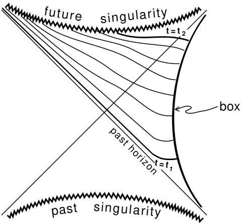
FIG. 4.:

REFERENCES

- [1] S. W. Hawking, Commun. Math. Phys. 43, 199 (1975).
- [2] J. M. Bardeen, B. Carter and S. W. Hawking, Commun. Math. Phys. 31, 161 (1973).
- [3] J. D. Bekenstein, Nuovo Cimento Lett. 4, 737 (1972); Phys. Rev. D 9, 3292 (1974).
- [4] N. D. Birrell and P. C. W. Davies, Quantum Fields in Curved Space, (Cambridge University Press, Cambridge, 1982).
- [5] L. Bombelli, R. Koul, J. Lee, and R. D. Sorkin, Phys. Rev. D 34, 373 (1986).
- [6] V. Frolov and I. Novikov, Phys. Rev. D 48, 4545 (1993).
-
[7]
M. Srednicki,
Phys. Rev. Lett. 71, 666 (1993);
G. ’t Hooft, Nucl. Phys. B256, 727 (1985);
L. Susskind and J. Uglum, Phys. Rev. D 50, 2700 (1994);
M. Maggiore, Nucl. Phys. B429, 205 (1994);
C. Callan and F. Wilczek, Phys. Lett. B333, 55 (1994);
S. Carlip and C. Teitelboim, Phys. Rev. D 51, 622 (1995);
S. Carlip, Phys. Rev. D 51, 632 (1995);
Y. Peleg, “Quantum Dust Black Holes”, Brandeis University report no. BRX-TH-350, hep-th/93077057 (1993). - [8] G. W. Gibbons and S. W. Hawking, Phys. Rev. D 15, 2752 (1977).
- [9] S. W. Hawking, in General Relativity: An Einstein Centenary Survey, edited by S. W. Hawking and W. Israel (Cambridge University Press, Cambridge, 1979).
- [10] J. W. York, Phys. Rev. D 33, 2092 (1986).
- [11] B. F. Whiting and J. W. York, Phys. Rev. Lett. 61, 1336 (1988).
- [12] B. F. Whiting, Class. Quantum Grav. 7, 15 (1990).
- [13] D. N. Page, in Black Hole Physics, edited by V. D. Sabbata and Z. Zhang (Kluwer Academic Publishers, Dordrecht, 1992).
- [14] J. Louko and B. F. Whiting, Class. Quantum Grav. 9, 457 (1992).
- [15] J. D. Brown and J. W. York, Phys. Rev. D 47, 1420 (1993).
- [16] J. Melmed and B. F. Whiting, Phys. Rev. D 49, 907 (1994).
- [17] T. Thiemann and H. A. Kastrup, Nucl. Phys. B399, 211 (1993); H. A. Kastrup and T. Thiemann, Nucl. Phys. B425, 665 (1994); T. Thiemann, Int. J. Mod. Phys. D 3, 293 (1994).
- [18] K. V. Kuchař, Phys. Rev. D 50, 3961 (1994).
- [19] J. Louko and B. F. Whiting, Phys. Rev. D 51, 5583 (1995).
- [20] J. D. Brown and J. W. York, Phys. Rev. D 47, 1407 (1993).
- [21] C. Teitelboim, Ann. Phys. (NY) 79, 524 (1973).
- [22] E. Witten, Phys. Rev. D 44, 314 (1991).
- [23] S. Bose, J. Louko, L. Parker, and Y. Peleg, Phys. Rev. D 53, 7089 (1996).