Teleparallel Space-Time with Defects yields Geometrization of Electrodynamics with quantized Charges

Abstract

In the present paper a geometrization of electrodynamics is proposed, which makes use of a generalization of Riemannian geometry considered already by Einstein and Cartan in the 20ies. Cartan’s differential forms description of a teleparallel space–time with torsion is modified by introducing distortion 1-forms which correspond to the distortion tensor in dislocation theory. Under the condition of teleparallelism, the antisymmetrized part of the distorsion 1–form approximates the electromagnetic field, whereas the antisymmetrized part of torsion contributes to the electromagnetic current. Cartan’s structure equations, the Bianchi identities, Maxwell’s equations and the continuity equation are thus linked in a most simple way. After these purely geometric considerations a physical interpretation, using analogies to the theory of defects in ordered media, is given. A simple defect, which is neither a dislocation nor disclination proper, appears as source of the electromagnetic field. Since this defect is rotational rather than translational, there seems to be no contradiction to Noether’s theorem as in other theories relating electromagnetism to torsion. Then, congruences of defect properties and quantum behaviour that arise are discussed, supporting the hypothesis that elementary particles are topological defects of space–time. In agreement with the differential geometry results, a dimensional analysis indicates that the physical unit $(lenght)^{2}$ rather than $As$ is the appropriate unit of the electric charge.

1 Introduction

Two independent developments led to the following considerations. In the early 50ies, Kondo [1] and independently Bilby et al. [2] discovered that topological defects in crystalline bodies, namely dislocations, have to be described in terms of differential geometry. Cartan’s torsion tensor was shown to be equivalent to the dislocation density. It was Kondo himself, who stressed in a series of papers [1] [3] that this discovery may have some impact beyond material science. Kröner completed the theory in an outstandingly clear way [4] [5] and obtained many results that remind us from electrodynamics. I the meantime, many researchers felt particulary attracted by the beauty of this theory which includes the mathematics of general relativity (GR) as a special case. With Kröner’s words: ” We have seen that Riemannian geometry was to narrow to describe dislocations in crystals. Is there a reason why space–time has to be described by a connection that is less general than the general metric–compatible affine connection ?”
The second reason for dealing with this topic is Einstein’s so–called teleparallelism attempt towards a unified field theory, grown out of the correspondence with Elie Cartan [6] and cumulating in an article in the Annalen der Mathematik in 1930 [7]. Even if this attempt did not succeed, the fact that Einstein, trying to create a unified theory of electrodynamics and gravitation, considered the same extension of Riemannian geometry that has shown to describe defect theory, remains a remarkable coincidence. Unfortunately, most physicits have associated Einstein’s belief in the existence of a unified theory in this context to his continuous objections to quantum mechanics. It is one of the main purposes of this paper to show that there is no contradiction between quantum mechanics and a differential geometry approach towards a unified theory. Other interesting congruences between quantum behaviour and facts emerging from geometry have been detected by Vargas [8] [9].

In section 2, the differential geometry of a 4–dimensional manifold is revisited in differential forms language using Cartan’s moving frame method that focusses on integrability conditions. By introducing distorsion 1-forms Maxwell’s equations appear as purely geometric identities. Thereby it is assumed that on a large scale, the Levi-Civita connection describes as usual GR, whereas a teleparallel connection governs physics on a microscopic level, generating two kinds of geodesics: extremals (depending on the metric only) and autoparallels. In section 2.7, some of Einstein’s tensor quantities are translated into modern forms language. Contrarily to Einstein’s conviction, this proposal allows singularities in space–time (topological defects). In section 3, a visualization of the obtained results by means of dislocation theory is given. The starting point is the Lorentz–invariance of the motion of dislocations, whereby the velocity of shear waves is analogous to the velocity of light. A generalization of dislocation theory with finite–size defects, which are described by homotopy theory, is needed for a physical interpretation of the quantity representing the current. Therefore, the proposed geometrization of electrodynamics seems to require a quantization of the electric charge. Further similarities of defect physics to quantum mechanis are discussed in section 4, at the present stage necessarily in a qualitative manner. In section 5, some dimensional analysis remarks about physical units and the calculability of masses are given. Although these remarks may not be considered sufficiently convincing for founding a physical theory by themselves, their implications fit to the previously developed results.
As more recent papers I took inspiration from I should mention Vargas’ papers on geometrization [10] [11] [12], Vercin [13], who discussed dislocations under the perspective of gauge theories, and Hehl [14], who gave a review of the use of torsion in general relativity relating the torsion tensor to spin. At the end of section 3, I will discuss the general objections formulated by Hehl[15] against relating electromagnetism to torsion and a possible solution.

2 Differential geometry of a 4–dimensional manifold with curvature and torsion

A scalar–valued $p$–form $\eta$ is called closed, if $d\eta=0$ ($d$ is the exterior derivative), and called exact, if a $(p-1)$–form $\zeta$ exists with $d\zeta=\eta$. The rule $dd=0$ implies exact $\Rightarrow$ closed. In other words, if $d\eta$ is a nonvanishing $(p+1)$–form, a $\zeta$ with the above property cannot be defined globally.

Regarding the vector– and tensor–valued forms occurring in the differential geometry of a 4–dimensional manifold the situation is not that simple. To get an overview, one may list the quantities which are the most important ones in the following sense (see in Tab. I):
If the $(p-1)$–forms can be defined globally, the respective $(p+1)$–forms have to vanish identically. These integrability conditions cannot be expressed by applying a differential operator as when dealing with scalar-valued forms. Furthermore, the integrability conditions link the vector–valued with the tensor–valued forms.

p-form	symbols	quantity	satisfies
0-form	$A^{\ \nu}_{\mu},A^{\nu}$	Lie group
1-form	$\omega_{\mu}^{\ \nu},\omega^{\nu}$	connection	structure equation
2-form	$R_{\mu}^{\ \nu},T^{\nu}$	field	Bianchi identity
3-form	$J_{\mu}^{\ \nu},J^{\mu}$	current	continuity equation
4-form		invariant	d=0

Table I.

2.1 Integrability conditions

Cartan [16] [17] developed the theory of affine connections starting from integrability conditions. He introduced the vector equation for a point ${\bf P}$ in an arbitrary fixed basis ${\bf a_{\mu}}$ as

$${\bf P}={\bf P}_{0}+A^{\mu}{\bf a_{\mu}},$$ (1)

whereas a frame is given by

$${\bf e_{\mu}}=A_{\mu}^{\ \nu}{\bf a_{\nu}}.$$ (2)

By differentiating the affine group with elements $(A^{\mu},A^{\ \nu}_{\mu})$ one obtains the pair $(\omega^{\mu},\omega_{\nu}^{\ \mu})$, the usual exterior derivative operator $d$ is here applied also to the basis ${\bf e_{\mu}}$ :

$$d{\bf P}=d({\bf P}_{0}+A^{\mu}{\bf a_{\mu}})=\omega^{\mu}{\bf e}_{\mu}$$ (3)

and

$$d{\bf e_{\nu}}=d(A_{\mu}^{\ \nu}{\bf a_{\nu}})=\omega_{\nu}^{\ \mu}{\bf e_{\mu}}.$$ (4)

$\omega_{\nu}^{\ \mu}$ stands for $B_{\kappa}^{\ \mu}dA_{\nu}^{\ \kappa}$ and $\omega^{\mu}$ for $B_{\kappa}^{\ \mu}dA^{\kappa}$, the matrix $B$ is the inverse of $A$. If we ask ourselves, whether the system (3-4) is integrable, the rule $dd=0$ yields the neccessary conditions, the Maurer-Cartan structure equations of a Lie group:

$$d\omega^{\lambda}-\omega^{\nu}\wedge\omega^{\ \lambda}_{\nu}=0,$$ (5)

and

$$d\ \omega_{\lambda}^{\ \kappa}-\omega_{\lambda}^{\ \nu}\wedge\omega^{\ \kappa}_{\nu}=0.$$ (6)

These are the integrability conditions for the system (3-4), the neccessary conditions for manifold to be locally affine space, thus the neccessary conditions for defining $A_{\mu}^{\ \nu}$ and $A^{\nu}$ globally. On the other hand, eqns. (5) and (6) will be used as definitions for torsion and curvature if the terms on the r.h.s. do not vanish. Torsion and curvature stand for the failure of integrability of the system (3) and (4).

2.2 Equations of structure and Bianchi identities

Going one level down in Tab. I, analougous arguments apply: rather than integrating the connections and obtaining the Lie group, the connections are now considered as the basic quantities. For example, in GR, the Riemannian curvature tensor is defined by

$$R_{\nu\mu\lambda}^{.\ .\ .\ \kappa}=\partial_{\nu}\Gamma_{\mu\lambda}^{\kappa}-\partial_{\mu}\Gamma_{\nu\lambda}^{\kappa}+\Gamma^{\kappa}_{\nu\rho}\Gamma^{\rho}_{\mu\lambda}-\Gamma^{\kappa}_{\mu\rho}\Gamma^{\rho}_{\nu\lambda},$$ (7)

where $\Gamma_{\mu\lambda}^{\kappa}$ is the Levi-Civita-connection. However, eqn. (7) holds as well for a more general affine connection which is not neccessarily symmetric in the lower two indices and not completely determined by the metric. In differential forms language, eqn. (7) is called the second structure equation and takes the form

$$R_{\lambda}^{\ \kappa}=d\omega_{\lambda}^{\ \kappa}-\omega_{\lambda}^{\ \rho}\wedge\omega^{\ \kappa}_{\rho},$$ (8)

using the antisymmetric properties of the exterior algebra and omitting the form indices in eqn. (7). Using differential forms language of Cartan puts in evidence the fundamental difference between the value indices $\lambda$ and $\kappa$ and the form indices $\mu$ and $\nu$ (eqn. 7). The latter define the surface on which a 2–form ‘lives’. $R_{\lambda}^{\ \kappa}$ is the curvature 2-form and $\omega_{\lambda}^{\ \kappa}$ is the connection 1-form, both of them take values in the Lie algebra of the affine group. To obtain the integrability conditions for the connections, one has to differentiate (8):

$$d\ R_{\lambda}^{\ \kappa}-\omega^{\ \kappa}_{\nu}\wedge R_{\lambda}^{\ \nu}-\omega^{\ \nu}_{\lambda}\wedge R^{\ \kappa}_{\nu}=0,$$ (9)

This is called the Second Bianchi identity. Analogously to (5) with nonvanishing r.h.s., one differentiatiates the vector-valued basis 1-forms $\omega^{\lambda}$, and obtains the torsion tensor:

$$T^{\lambda}=d\omega^{\lambda}-\omega^{\nu}\wedge\omega^{\ \lambda}_{\nu},$$ (10)

which is called first structure equation. The integrability conditions for the basis 1–forms are obtained by differentiation of the vector-valued 2-form torsion:

$$d\ T^{\kappa}+T^{\nu}\wedge\omega^{\ \kappa}_{\nu}-\omega^{\nu}\wedge R^{\ \kappa}_{\nu}=0,$$ (11)

which is called First Bianchi identity. The Bianchi identities are the integrability conditions the fields have to satisfy in order to yield well–defined connections. If torsion and curvature are chosen independently without satisfying the Bianchi identities, the pair of connections $(\omega^{\mu},\omega_{\nu}^{\ \mu})$ cannot be defined any more. In the following, we will investigate the interplay of the two branches that led to the 1st and second Bianchi identity. In a situation with vanishing curvature, i.e. breaking only the integrability conditions for the vector equation, one can still integrate eqn. 6 and obtain a globally defined frame ${\bf e}_{\mu}$, whereas the opposite constraint, curvature with zero torsion like in GR, does not even allow the integration of eqn. 5, because the nonintegrable frame ${\bf e}_{\mu}$ ‘spoils’ also eqn. 5.
In conclusion, one may, discarding the connections, descend further in Tab. I and consider the integrability conditions for the fields: the currents $J_{\mu}^{\ \nu}$ and $J^{\nu}$ , now defined as the nonvanishing r.h.s. of (9) and (11) still have to satisfy their continuity equations (vanishing 4-forms in Tab. I) in order to yield well–defined fields. Since this extension is not neccessary for the following, I will not go into details here.

2.3 Teleparallel description of General Relativity

In the following we restrict to a metric-compatibile connection ($\omega_{\mu\nu}+\omega_{\nu\mu}=0$). Then, I will consider a teleparallel geometry, that means the curvature 2–form $R_{\lambda}^{\ \mu}$ vanishes everywhere. This does not inhibit a geometric description of the energy-momentum tensor, rather it can be seen as a formal replacement of the Levi–Civita connection by a teleparallel connetion. Since there is a freedom in choosing the connection this can always be done by adding to $\Gamma_{\mu\nu}^{\kappa}$ the so–called contorsion tensor [19] [20]

$$S_{\mu\nu}^{\ \ \kappa}:=T_{\mu\nu}^{\ \ \kappa}-T_{\nu\ \mu}^{\ \kappa}+T_{\ \mu\nu}^{\kappa},$$ (12)

where $T_{\mu\nu}^{\ \ \kappa}$ are the components of torsion. In this case the Riemannian curvature tensor of GR (which is obtained from the Levi–Civita connection) can be expressed in terms of torsion and its derivatives (cfr. [19], 4.22). In this case, the usual geodesics (extremals determined by the metric only) have to be distinguished from autoparallels.

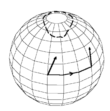
Figure 1: If autoparallels on the unit sphere are defined according to the Mercator projection, one obtains a teleparallel structure with vanishing curvature. The parallel transported vector changes direction in the imbedding 3-dimensional space, whereas the angle to the meridians is kept fixed.

To illucidate the interplay curvature–torsion, the simple example Fig. 1 (cfr.[21], sec.7.3) is given. The ususal geodesics (extremals) on a sphere are great circles, but one may alternatively define parallel transport by keeping the angle between the vector and the straight line in Mercator’s projection fixed. The geometry becomes teleparallel, but has nonzero torsion. The meridians are in this case autoparallels rather than geodesics determined by the metric (extremals). Transporting a vector along a closed path around one of the poles (see dotted line in Fig. 1), however, yields a whole turn of $2\pi$. We may regard the two poles as having Dirac-valued curvature. In this case, integrating the curvature over the whole sphere still yields $4\pi$, as required by the Gauss-Bonnet theorem.
These topological issues were addressed first by Cartan in his letter to Einstein from Jan 3, 1930 [6]: ‘Every solution of the system (6) creates, from the topological point of view, the continuum in which it exists’ .

2.4 The distortion 1–forms $\theta^{\mu}$

In conventional tensor analysis, traces are important because they are invariant under coordinate transformations. The same holds for the antisymmetric part of a tensor. In differential forms language, the latter corresponds to exterior multiplication with the basis 1-forms $\omega^{\mu}$, whereby the sum over the doubled index $\mu$ is taken. This antisymmetry operator ${\cal A}$ that raises the degree of a form, but lowers the degree of the value indices, whereas the exterior derivative $d$ raises the degree of a form, without changing the type of the form (tensor-, vector-valuedness).
If we investigate the equations of 2.2, we may visualize the respective contributions of these operators to the quantities in Tab. I in the following sketch:

Figure 2: From top to bottom, the degree of the respective differential forms increase; from left to right, the number of value indices decreases. The $p$-forms exist only, if the respective $(p+2)$-form vanishes.

By the action of ${\cal A}$ the connection 1–form is transformed into a vector valued 2–form (which is, in the holonomic case, torsion); the tensor–valued Riemannian curvature 2–form is transformed into a vector–valued 3–form $\omega^{\nu}\wedge R^{\ \kappa}_{\nu}$ which contributes to the ‘current’ of torsion $J^{\mu}$. We may formally extend this action of the antisymmetry operator to the ‘top level’ of the left column in Fig. 2, the 0–form $A_{\mu}^{\ \nu}$ which takes values in the linear group, and consider besides $\omega^{\nu}$ the term

$$\theta^{\nu}:=\omega^{\nu}-\omega^{\mu}\wedge A_{\mu}^{\ \nu}$$ (13)

or briefly $\omega^{\nu}-dA^{\nu}$, which I shall call distortion 1–form, referring already to the physical interpretation given in section 3. In Euclidean space, one could write

$$\theta^{\nu}=B_{\kappa}^{\ \nu}dA^{\kappa}-A_{\mu}^{\ \nu}\wedge B_{\kappa}^{\ \mu}dA^{\kappa}=(B_{\kappa}^{\ \nu}-\delta_{\kappa}^{\ \nu})dA^{\kappa},$$ (14)

where $\delta_{\mu}^{\ \nu}$ is the Kronecker delta (0–form). It follows easily that $d\theta^{\nu}=d\omega^{\nu}$. Therefore, the first Bianchi identity is not affected if in the first structure equation $d\omega^{\lambda}$ is replaced by $d\theta^{\lambda}$. This definition takes into account that $dA_{\mu}^{\ \nu}$ and $dA^{\mu}$ are different quantities that should consequently be ‘transformed back’ also by different quantities $B_{\nu}^{\ \mu}$ and $(B_{\mu}^{\ \nu}-\delta_{\mu}^{\ \nu})$. Cartan frequently called $(\omega^{\mu},\omega_{\nu}^{\ \mu})$ the pair of connections. In a certain sense it is more justified to call $(\theta^{\mu},\omega_{\nu}^{\ \mu})$ the pair of connections since both $\theta^{\mu}$ and $\omega_{\nu}^{\ \mu}$ can be brought to zero locally by an appropriate Lorentz transformation.

Figure 3: The basis 1-forms $\omega^{\mu}$ in Fig. 2 are replaced by the deformation 1-forms $\theta^{\mu}$. The extension of the relations in Fig. 2 leads to Maxwell’s 2nd pair of equations as Bianchi identity in the ‘0th’ column to the right.

2.5 Maxwell’s equations

In the most general situation outlined in Fig. 3, I consider again a teleparallel geometry with a vanishing curvature 2–form $R_{\lambda}^{\ \mu}$, that means the connection $\omega_{\mu}^{\ \nu}$ is integrable and the 0-forms $A_{\mu}^{\ \nu}$ can be defined in every point of the manifold.
A straightforward extension of the relations in Fig. 2 is applying the antisymmetry operator to the distortion 1-forms $\theta^{\mu}$ (Since $\omega^{\mu}\wedge\omega_{\mu}$ is zero, this would have been senseless without introducing $\theta^{\nu}$), which is equivalent to applying the antisymmetry operator with respect to both indices of $A_{\mu}^{\ \nu}$:

$$F^{*}:=-\omega_{\nu}\wedge\theta^{\nu}=A_{\mu}^{\ \nu}\wedge\omega_{\nu}\wedge\omega^{\mu}.$$ (15)

For reasons that will become clear soon I call the resulting 2-form $F^{*}$, the tensor dual to the electromagnetic field. Exterior differentiation yields

$$J^{*}:=dF^{*}=d\theta^{\mu}\wedge\omega_{\mu}-\theta^{\mu}\wedge d\omega_{\mu}.$$ (16)

with the 3-form $J^{*}$. Analogous to the other relations in Fig. 3, the antisymmetrized torsion $T^{\mu}\wedge\omega_{\mu}$ contributes to $J^{*}$ .
As the reader may have noted, one can now obtain Maxwell’s 2nd pair of equations $\delta F:=*d*F=J$ by identifying the 2-form $F^{*}$ with the dual of the electromagnetic field 2-form $F$ and by identifying $J^{*}$ with the 3–form dual to the current $J$. Poincare’s lemma $dd=0$, applied to $F^{*}$, yields the continuity equation. Both equations appear in the ‘0th column’ to the right of Fig. 3 as Bianchi identity and continuity equation .
Eqn. 16, written as $\delta F=J$ does not determine completely the 2–form $F^{*}$. The remaining degree of freedom can be used to satisfy Maxwell’s 1st pair of equations, $dF=0$, or equivalently, by introducing the vector potential $A$ with $dA=F$. One should not forget, however, that due to deRham’s theorem, there is still a degree of freedom left for $F$, since every harmonic form $H$ satisfies $dH=\delta H=0$. Therefore, $F$ is only determined up to a harmonic form.

2.6 Nonlinearity

The $A_{\mu}^{\ \nu}$ are elements of $GL(4)$. If we consider the subgroup $GL(3)$, antisymmetrizing the elements of $GL(3)$ with ${A_{\mu}^{\ \nu}\wedge\omega_{\nu}\wedge\omega^{\mu}}$ corresponds (up to a double cover) to a projection on $SO(3)$ and a linearization. The $A_{\mu}^{\ \nu}$ give information about the distorsion (dilatation and shear) and orientation of a volume element with respect to a given coordinate system, the ${A_{\mu}^{\ \nu}\wedge\omega_{\nu}\wedge\omega^{\mu}}$ about the orientation only.
$SO(3)$ is a deformation retract of the nonsingular elements of $GL(3)$. Applying the antisymmetry operator with respect to both indices means projecting from $GL(3)$ to $SO(3)$, with the restriction that the resulting term appears in the vesture of a 2-form which can be written as an antisymmetric matrix. Thus in first approximation, multiplication of $SO(3)$-matrices can be done by adding their antisymmetric parts, that means, in first approximation, one may describe the electromagnetic field as a 2-form, and in first approximation, the superposition principle holds.

2.7 Relations to the Einstein-Cartan TP attempt

The above considerations on $A_{\mu}^{\ \nu}\wedge\omega_{\nu}\wedge\omega^{\mu}$ were inspired by Einstein’s 1930 paper. I will explain which of Einstein’s tensor quantities correspond to forms in the above sections, referring to equation numbers there [7].

Einsteins vierbeins $h_{s}^{\nu}$ (section 2) correspond to $A_{\mu}^{\ \nu}$. Eqn.(12), though in tensor language, is equivalent to the definition of the $\omega_{\mu}^{\ \nu}$ I repeated in section 2.1 (he writes both $h$ for the Matrix and its inverse). I should say here that I do not propose Einsteins (29) and (30), together with their definitions (27) and (28), as field equations. (27) may be seen as interior covariant derivative of torsion (cfr. [26]) but (28) does not define a reasonable quantity from the differential forms perspective.

In his section ‘first approximation’, Einstein considers the quantities $\bar{h}_{s}^{\nu}$ defined in (37). To translate this into forms language, I introduced the $\theta^{\nu}$’s in section 2.4. The $\theta^{\nu}$’s, however, are not neccessarily small as $\bar{h}_{s}^{\nu}$ is small compared to $h_{s}^{\nu}$. If we go ahead, Einstein considers the antisymmetric part of the $\bar{h}_{a\mu}$, $\bar{a}_{a\mu}$ (eqn. 45). Since the only possible ‘translation’ of $\bar{a}_{a\mu}$ is $A_{\mu}^{\ \nu}\wedge\omega_{\nu}\wedge\omega^{\mu}$, Einstein’s ‘electromagnetic field’ $\bar{a}_{a\mu}$ coincides with the quantity $F^{*}$ I proposed as dual to the electromagnetic field.

3 An elastic continuum with defects as model for a space–time with particles

Differential geometry has shown to describe the physics of defects [1] [2] [4] [5]. Cartan’s structure equations and the Bianchi identities are the natural nonlinear generalizations of the definitions and the governing equations in defect theory [13]. For example, the first Bianchi identity expresses the fact that dislocations may not end inside a crystalline body (teleparallelism). I will now use dislocation theory for visualizing the above results. Since in a dislocated crystal directions of vectors may be compared globally, it can be described by a teleparallel geometry discussed in the previous section. It is clear that the physics of defects in a real crystal cannot be completely equivalent to the physics of space–time, but one may use the concept of the ‘continuized crystal’ [5] it as a model providing further insight. It will be helpful here to be familiar with the concept of the ‘internal observer’ in a crystal introduced by Kröner [5], see also [27]. The internal observer measures distances by counting lattice points. He is unable to detect deformations or waves of the elastic space-time-continuum, as long those do not manifest themselves in defects. The most important presupposition for a spacetime-analogy, however, is the appropriate description of Lorentz–invariance.

3.1 Lorentz-invariance in dislocation theory

The discovery of a relativistic behaviour of dislocations goes back to Frank [28] and Eshelby [29] in 1949. They showed that when a screw dislocation moves with velocity $v$ it suffers a longitudinal contraction by the factor $\sqrt{1-\frac{v^{2}}{c^{2}}}$, where $c$ is the velocity of transverse sound. The total energy of the moving dislocation is given by the formula $E=E_{0}/\sqrt{1-\frac{v^{2}}{c^{2}}}$, where $E_{0}$ is the potential energy of the dislocation at rest. These old, but exciting results were recently extended [30] [31] to a Lorentz-invariant theory of defect dynamics. In real media, two velocities for longitudinal and transversal sound exist. This was considered as an obstruction by several authors [32] [33] to a complete analogy between a continuum with defects and space-time with matter, since longitudinal sound is always faster and two different $c$’s would ‘destroy’ the relativistic description. However, space–time can be assumed to be ‘incompressible’. If one goes to the limit of infinite velocity for longitudinal sound, the formulas (12) and (13) in [29] yield only distorsions of shear type. Since every defect causes also shear distorsions, it causes shear distorions only in the limit of incompressibility. Therefore no defect defect matter may propagate faster than the velocity of transverse sound, otherwise its energy would become infinite.
Since space–time is no ordinary matter, there is no physical contradiction in the assumption of incompressibility. Therefore, following [13], defect dynamics may be described formally in a 4–dimensional space–time with torsion and Lorentzian signature of the metric.

3.2 The most simple defect – an electron ?

There are two distinct types of dislocations, screw and edge dislocations, each of them causing different distorsions of the crystal. From this follows that there is a certain separability of the physics of screw and edge dislocations. Of particular interest are here screw dislocations, because the expression obtained above by antisymmetrizing the torsion tensor gave a contribution to the current $J^{*}$. Torsion is equivalent to the dislocation density tensor $\alpha_{\kappa\mu}^{\ \ \lambda}$ and the density of screw dislocations is described by mixing the indices $\kappa\mu\lambda$, this is sometimes called H-torsion.

Before going further in relating the two types of dislocations to electromagnetism and gravitation, one has to realize that dislocations are line singularities, whereas elementary particles are expected to be point-like defects. Therefore, we are interested in finding the most simple possible defects in an elastic continuum that (at least macroscopically) appear as point-like. Since dislocations cannot end within the crystal unless there is curvature, it is an immediate guess to consider closed dislocation loops. The problem is that in crystals no closed screw dislocation loops exist. Rather closed loops of dislocations consist of two pairs of screw and edge dislocations of opposite sign each other . This defect can be visualized by cutting the continuum along a surface, displacing the two faces against each other by the amount of the Burgers vector and rejoining them again by gluing.
Similarly we can think of cutting a (circular) surface, twisting the faces, and gluing them together again (see Fig. 4). This would correspond to a closed screw dislocation loop, but a crystal lattice resembling distant parallelism cannot be defined any more.

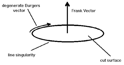
Figure 4: A screw dislocation has a Burgers vector parallel to the dislocation line. The defect depicted here is locally equivalent to a screw dislocation, if the twisting (Frank) vector is small, otherwise the Burgers vector degenerates to a curved object.

In another context, this kind of defect has been investigated by Huang and Mura [36], who called it edge disclination, referring to disclination theory. The twisting angle is called Frank vector there. If a vector is transported parallely along a path going through this ‘screw dislocation loop’, the twisting would yield a nonvanishing Riemannian curvature tensor (which indeed, describes defects in disclination theory).
In the case the ‘screw dislocation loop’ is a Dirac–valued line singularity of finite size, one can resolve, however, the problem by allowing only multiples of $2\pi$ as twisting angles, thus maintaining the teleparallel structure. Precisely this defect has been described by Rogula [37], who consideres it a ‘third’ type of defect which is neither a dislocation nor a disclination. For the following reasons I consider this defect a good candidate for describing the electron:

• On the large scale, its defect density becomes approximated by the (antisymmetrized) H-torsion, which gives a contribution to the current $J^{*}$ in section 2.5.

• The defect is a source of the deformation that corresponds to the electric field.

• Two versions of this defect exist, which according to its screwsense, could represent an electron or positron. This ‘handedness’ of the defect would explain CP-violation.

• H-torsion couples to spin $1/2$-fields [38] [39] [40].

3.3 Description by means of homotopy theory

Topological defecs are classified by homotopy groups. If we look at the static case of three dimensions, line defects are described by the fundamental group $\pi_{1}$, whereas the second homotopy group $\pi_{2}$ classifies point defects.
In terms of principal fibre bundles, during parallel transport along a path a vector undergoes a transformation, which is in the above case an element of the fibre $SO(3)$. The closed path through the ‘screw dislocation loop’ yields a whole rotation by an angle of $2\pi$, corresponding to a nontrivial element of the first homotopy group of the fiber $SO(3)$. Since $\pi_{1}(SO(3))$ is ${\sf Z\kern-4.5ptZ}_{2}$, we face the problem that two defects, each of them representing an electron, cancel out by the rule $1+1=0$. Coiled line defects, however, do influence also higher homotopy groups (for example $\pi_{2}$ is influenced by $\pi_{1}$ of the projective plane, see [21] [41]).
Since in the case of $SO(3)$ $\pi_{2}$ is $0$, no topologically stable point defects may exist. The solution to this dilemma may be a defect called Shankar’s monopole [42], representing the the nontrivial element $1$ of the third homotopy group $\pi_{3}(SO(3))$, which is ZZ.
Considering their ‘screwsense’, it is impossible that two ‘screw dislocation loops’ could merge in a way that makes the distorsion of the continuum disintegrate completely. I suppose rather that two ‘screw dislocation loops’ form a Shankar monopole. In this case, $\pi_{1}$ vanishes, but $\pi_{3}$ (rather than $\pi_{2}$) would be influenced by the fundamental group $\pi_{1}$.

3.4 Some implications and objections

Given the approximation in section 2.5, the 0th component of the 3-form H-torsion is proportional to the amount of area enclosed in the ‘screw dislocation loop’, since the length of the dislocation – assuming multiples of $2\pi$ as Frank vector – is multiplied with a ‘degenerate’ Burgers vector, whose length is again proportional to the length of the loop. Therefore, charge can be seen as the amount of ‘twisted area’ of all defects in a volume, regardless their directions of the Frank vector. To ease understanding, only the static 3-dimensional case of screw dislocations was discussed here, which corresponds to the 0th component of the 4-dimensional current (charge). One should, however, remember, that the Lorentz-invariant properties of defect dynamics allow a formal description in 4 dimensions. Therefore components involving time should behave alike.

The electromagnetic field, according to this proposal, takes values in the Lorentz group, $SO(3,1)$, a pure electric field in the subgroup $SO(3)$. This sounds very strange, since the entire electromagnetic field, not only the purely electric or magnetic part could vanish under Lorentz transformations. This does, however, hold only locally. If we consider of the ‘closed screw dislocation loop’ which, according to its screwsense, represents an electron or positron, its inside is rotated by a amount of $\pi$ relative to a point at infinite distance where the electric field vanishes. A rotation of the coordinate system could make the inside and vicinity of the electron nearly field–free but would cause a homogenous electric field of (maximum) value $\pi$ far from the defect. Therefore, such a transformation changes not only the electromagnetic field but also the nature of its test particles in a manner that leaves the physical situation unchanged. In other words, the topology of a space–time with these defects generates a preferential coordinate system, according to which we usually define the electromagnetic field.

A serious objection against theories relating torsion to electromagnetism is the following: Torsion is related to translations and translations are related to energy-momentum via Noether’s theorem, ‘and nothing else’, as Hehl [15] states. In the present proposal, the electromagnetic field is related to the quantity ${A_{\mu}^{\ \nu}\wedge\omega_{\nu}\wedge\omega^{\mu}}$ (cfr. sec. 2), which does not contain torsion. I suggested, however, that the antisymmetrized torsion ${T^{\nu}\wedge\omega_{\nu}}$ contributes to the electromagnetic current. Being a $3$-form, it is not reasonable to integrate this quantity over a surface, as one does with the torsion $2$-form which yields then a translation.

Furthermore, H-torsion is only an approximation for the defect density. The ‘closed screw dislocation’ defect proposed as elementary particle of the current, is, as Rogula [37] explains, a defect of its own type. From the arguments in section 3.2 it is obvious that it is a rotational defect rather than a translational one. Therefore, Noether’s theorem seems not to contradict this proposal. On the other hand, if torsion can serve as an approximation only, a precise differential geometric descrition of the above defect is desirable.

4 Quantum behaviour of defects

It is interesting that the restriction of teleparallelism, that led to Maxwell’s equations in section 2.6, applied to dislocation theory, led to a quantization of the term $T^{\nu}\wedge\omega_{\nu}$ which contributes to the electric charge.

Topological defects, however, share most interesting properties with the quantum behaviour of particles. Firstly, a sign change in the homotopic classification of a defect describes an ‘antidefect’, corresponding to the phenomenon of every particle having an antiparticle. This allows an obvious and intuitive understanding of the pair creation and pair annihilation processes.

Fig. 5 a) shows how the motion of a single dislocation in a crystal from Point $P$ to $Q$ is indistinguishable from a process that involves an anihilation of two dislocations of opposite sign in $A$ and a creation of two dislocations in $C$.

Figure 5: The propagation of dislocations, ‘screw disloaction loops’, or electrons is completely analogous. By measuring the events in $P$ and $Q$, there is no method to detect whether a defect propagating from $P$ to $Q$ goes a ‘direct’ path (a) or has a creation–anihilation process plugged in between (b). The ‘Feynman diagrams’ (a) and (b) are indistinguishable.

Analagously, if we interpret the defects in Fig. 5 as ‘screw dislocation loop’ and its inverse (electron and positron), it can be seen as Feynman Diagram with two an extra couplings (an additional virtual photon travels from $A$ to $C$ backwards in time).

If one measures only the ‘departure’ of an electron in $P$ and the ‘arrival’ in $Q$, it is clear that it makes no sense to speak about a trajectory of an elementary particle. Considering the double slit experiment it makes no sense to say the defect went the one way or the other. This famous consequence of the quantum mechanics does not appear mysterious any more.

Then, topological defects themselves are as indistinguishable, if their homotopic classification coincides. As elementary particles, one cannot describe them with classical statistics.

In such a space–time, only defects are detectable. I refer here again to the concept of the ‘internal observer’ in a crystal introduced by Kröner [5]. Any quantum mechanical observer is an ‘internal observer’ in this sense. He may by no means detect distorsions or waves of the elastic space-time-continuum, as long those do not manifest themselves in defects. Defects cannot be described properly as waves only, nor being classical particles. Rather a field may be seen as a ‘tendency to generate defects’.

If space–time is distortable, one may assume that under large or enduring stress, it ‘wrenches’ and builds defect pairs. The tendency to produce these topological defects should be governed by the value of Planck’s constant $h$. Regarding determinism, a ‘background temperature’ consisting of oscillations of the elastic continuum may cause non predictable random fluctuations of the equations of motion on a microscopic level (vacuum fluctuations). Thus complete determinism would be impossible as a matter of principle.

5 Dimensional analysis

Dimensional analysis,the method on which the following remarks are based, has been developed by Bridgeman [43]. Recent work in analysing unification theories by considering fundamental constants was done by [44], [45], [46] and [47].

5.1 Definitions

There is an analogy between vectors in a n-dimensional vector space and fundamental constants. $n$ vectors $v_{i}$ are linear independent if

$$\sum_{i=1}^{n}a_{i}v_{i}=0$$ (17)

implies $a_{i}=0$ for all $i$. Let’s call $dim(c)$ the SI units of an expression $c$ containing fundamental constants. The Operator $dim$ defines an equivalence relation, for example $n~{}\cong~{}1$ holds for any real number $n$.
$n$ fundamental constants $c_{i}$ are called independent, if from

$$dim(\prod_{i=0}^{n}c_{i}^{\gamma_{i}})=1,$$ (18)

$d_{i}\in{\rm R}$, follows $\gamma_{i}=0$ for all $i$. For example, the speed of light $c$, dielectricity $\epsilon$ and permeability $\mu$ are not independent because $\mu\epsilon$= $\frac{1}{c^{2}}$. A set of fundamental constants generates a space of SI units; from $h$, $G$ and $c$ we obtain by a ‘basis transformation‘ the SI units $m$, $kg$, $s$:

$$\left(\begin{array}[]{cc}m\\ s\\ kg\\ \end{array}\right)\cong\left(\begin{array}[]{c}-3/2\quad 1/2\quad 1/2\\ -5/2\quad 1/2\quad 1/2\\ \quad 1/2\quad 1/2-1/2\end{array}\right)\left(\begin{array}[]{c}c\\ h\\ G\end{array}\right).$$ (19)

where the matrix elements denote exponents. Addition in the common matrix algebra is replaced by multiplication. The thus obtained units are known as Planck’s units.

5.2 The vector space of fundamental constants

I will prove now :
$kg$ $\notin$ span($h$, $c$, $\epsilon$, $e$).
Proof:$h$, $c$, $\epsilon$, $e$ are dependent, because

$$dim(\frac{e^{2}}{h\/c\/\epsilon})\cong 1,$$ (20)

because the fine structure constant $\alpha$ is dimensionless. It follows span($h$, $c$, $\epsilon$, $e$)= span($h$, $c$, $e$), because ($h$, $c$, $e$) are independent. If

$$dim(h^{\alpha}c^{\beta}e^{\gamma}kg^{\delta})=1,$$ (21)

then $\gamma=0$, because there is no way of getting rid of the Ampères. While the ligth speed $c$ transforms $s$ into $m$ only, the $m^{2}$ in the denominator of dim(h) can never be compensated by any power $\alpha$, $\beta$ and $\delta$ . Therefore, $\alpha=\beta=\delta=0$ follows.
Given the present unit system, any formula for the electron mass involves necessarily $G$.
This gives some evidence that a unification of electromagnetism and quantum theory could only be achieved in the context of general relativity, and therefore differential geometry. For several reasons, however, I doubt that - holding up the present physical unit system - a unified theory that predicts masses could be obtained at all:

• There are basically two possibilities of obtaining mass from the set $h$, $c$, $\epsilon$, $e$ and $G$: $\sqrt{\frac{e^{2}}{\epsilon G}}$ and $\sqrt{\frac{hc}{G}}$. The first does not contain $h$ and can therefore not resemble quantum behaviour, whereas the latter has neither $e$ nor $\epsilon$, consequently no electrodynamics in it.

• Both expressions differ by 20 orders of magnitude from the electron mass. It is very unlikely that a unifying theory can give a simple formula for a factor $10^{20}$. A similar remark was given in [48].

• It would be still an open question to calculate the electromagnetic part of the electron mass (an expression, that obviously should not involve $G$).

The electromagnetic units Ampère, Volt etc. are rather arbitrary. Let us remind that at Maxwell‘s time Coulumb’s law was written $F=\frac{e^{2}}{r^{2}}$, and therefore $dim(e)=\sqrt{\frac{kgm^{3}}{s^{2}}}$ or $m\sqrt{N}$. These conventions obviously do not change physics (with the old system one can’t calculate masses either, of course). It does not matter whatever unit one chooses for the elementary charge. Therefore, without doing any harm, a ‘purely geometric’ unit like $m^{2}$ can be defined as measuring charge. The units of physical quantities would change as follows:

Quantity	present units	new units
Charge	$As$	$m^{2}$
Current	$A$	$m^{2}s^{-1}$
Potential	$V$	$Nm^{-1}$
Dielectricity($\epsilon$)	$AsV^{-1}m^{-1}$	$m^{2}N^{-1}$
Permeability($\mu$)	$VsA^{-1}m^{-1}$	$kgm^{-3}$
Electric field	$Vm^{-1}$	$Nm^{-2}$
Magnetic field	$Vsm^{-2}$	$Nsm^{-3}$
Magnetic flux	V $s$	$Nsm^{-1}$

Table 2.
As one can easily verify, all physical laws remain unchanged. Of course, the choice of $m^{2}$ is motivated by the fact that the antisymmetric part of torsion, like torsion itself, has the physical unit $m^{-1}$, or $m^{2}$ per volume. Looking at Fig. 3, all quantities on topleft – bottomright diagonals have the same physical units. By modifying the unit system in the proposed manner, one gaines the possibility of obtaining a formula of the electron self-energy, for example $\frac{hc}{\sqrt{e}}$ - without $G$. If one relates this order of magnitude to the experimental value $E_{el}=0.511MeV$, the electron can be assumed to be a topological defect (as described in section 3.2) of the order $10^{-24}m^{2}$, the square of Compton’s wavelength. This is certainly be more realistic than the Planck length of $10^{-35}m$, but can hardly be tested unless an experimental method for determining the size of the topological defect is developed. If, however, other types of defects representing neutrons and protons can be found, a prediction of mass ratios should be possible if one assumes that the sizes of the respective defects (in $m$ or $m^{2}$) have simple ratios.

6 Outlook

The Lorentz-invariance in defect dynamics has only be proven rigidly for straight screw disocations. Although the defects described here can be expected to behave in the same manner, a (much more complicated) proof has still to be given.
To derive equations of motion, Lagrange densities have to be found. Until now, a defect description has only been proposed for the electron, not for the neutron and the proton. The success or failure of the present theory will depend on the possibility of finding a model also for the latter elementary particles.
The possibility of calculating self–energies of elementary particles, however, does not seem remote, since the electromagnetic field, taking values in $SO(3,1)$, is finite everywhere. Unfortunately, the lack of experimental methods for measuring the ‘radius’ of the electron does not allow a testable prediction. Additional models for other particles should, however, lead to a prediction of the respective mass ratios. Furthermore, the violation of the superposition principle for electromagnetic fields may be tested experimentally.
The main conceptual advantage of defect theory is that many properties of elementary particles to which we are familiar from experiments, like pair creation and anihilation, quantum statistics, wave–particle dualism, antiparticles, CP violation, nonexistence of radial symmetry and others appear to have a certain logical interplay.

Acknowledgement

I am grateful to Dr. Karl Fabian for guiding my attention to Prof. Kröner’s work. I owe a lot to Prof. Josè G.Vargas for teaching me Cartan’s moving frame method and for commenting on a first version of this paper.

References

- [1] K. Kondo. RAAG Memoirs of the unifying study of the basic problems in physics and engeneering science by means of geometry, volume 1. Gakujutsu Bunken Fukyu-Kay, Tokio, 1952.
- [2] B.A. Bilby, R. Bullough, and E. Smith. Continous distributions of dislocations: a new application of the methods of non-riemannian geometry. Proc. Roy. Soc. London, Ser. A, 231:263–273, 1955.
- [3] K. Kondo. RAAG Memoirs of the unifying study of the basic problems in physics and engeneering science by means of geometry, volume 2. Gakujutsu Bunken Fukyu-Kay, Tokio, 1955.
- [4] E. Kröner. Allgemeine Kontinuumstheorie der Versetzungen und Eigenspannungen. Arch. Rat. Mech. Anal., 4:273–313, 1960.
- [5] E. Kröner. Continuum theory of defects. In R. Balian et al., editor, Les Houches, Session 35, pages 215–315. North Holland, Amsterdam, 1980.
- [6] R. Debever. Elie Cartan- Albert Einstein: Letters on Absolute Parallelism. Princeton University Press, 1979.
- [7] A. Einstein. Auf die Riemann-Metrik und den Fernparallelismus gegründete einheitliche Feldtheorie, english translation available under http://www.lrz-muenchen.de/ u7f01bf/www/einstein1930.intro.html. Mathematische Annalen, pages 685–697, 1930.
- [8] J.G. Vargas, D.G. Torr, and A. Lecompte. Geometrization of physics with teleparallelism. II. Towards a fully geometric Dirac equation. Foundations of Physics, 22(4):527–547, 1992.
- [9] J. G. Vargas and D. G. Torr. The construction of teleparallel Finsler connections and the emergence of an alternative concept of metric compatibility. Foundations of Physics, 27:825, 1997.
- [10] J.G. Vargas. Conservation of vector-valued forms and the question of existence of gravitational energy-momentum in general relativity. General Relativity and Gravitation, 23(6):713–732, 1991.
- [11] J.G. Vargas. Geometrization of physics with teleparallelism. I. The classical interactions. Foundations of Physics, 22(4):507–526, 1992.
- [12] J.G. Vargas and D.G. Torr. Finslerian structures: The Cartan-Clifton method of the moving frame. Journal of Mathematical Physics, 34(10):4898–4913, 1993.
- [13] A. Vercin. Metric–torsion gauge theory of continuum line defects. International Journal of Theoretical Physics, 29(1):7–21, 1990.
- [14] F.W. Hehl, G.D.Kerlick, P.v.d.Heyde, and J.M. Nester. General relativity with spin and torsion: foundations and prospects. Review of Modern Physics, 48:393–416, 1976.
- [15] F. W. Hehl and F. Gronwald. On the gauge aspects of gravity. e-Print Archive, http://xxx.lanl.gov/abs/gr-qc/9602013, 1985.
- [16] E. Cartan. C.R. Akad. Sci., 174:593, 1922.
- [17] E. Cartan. C.R. Akad. Sci., 174:734, 1922.
- [18] F.W. Hehl, W.Kopczynski, J.D.McCrea, and E.W.Mielke. Chern–Simons terms in metric affine space–time: Bianchi identities as Euler–Lagrange equations. Journal of Mathematical Physics, 32:2169–2180, 1991.
- [19] J.A. Schouten. Ricci-Calculus. Springer, New York, 1954.
- [20] F.W. Hehl and B.K. Datta. Nonlinear spinor equation and asymmetric connections in general relativity. Journal of Mathematical Physics, 12:1334–1339, 1971.
- [21] M. Nakahara. Geometry, Topology and Physics. IOP Publishing, 1995.
- [22] J. G. Vargas and D. G. Torr. The emergence of a Kaluza-Klein microgeometry from the invariants of optimally Euclidean Lorentzian spaces. Foundations of Physics, 27:533, 1997.
- [23] A. Einstein. Theorie unitaire du champ physique. Annales de l’institut Henri Poincare, 1:1–24, 1930.
- [24] E.W. Mielke. Ashtekar’s new variables in general relativity and its teleparallelism equivalent. Foundations of Physics, 219:78–108, 1992.
- [25] O. Candia and J. Zanelli. Torsional topological invariants. http://xxx.lanl.gov/abs/hep-th/9708138, 1997.
- [26] J. G. Vargas. Preprint, 1997.
- [27] L. Mistura. Cartan connection and defects in Bravais lattices. Int. Journal of Theoretical Physics, 29:1207–1218, 1990.
- [28] C.F. Frank. On the equations of motion of crystal dislocations. Proceedings of the Physical Society London, A 62:131–134, 1949.
- [29] J. Eshelby. Uniformly moving dislocations. Proc. Roy. Soc., Ser. A, 62:307–314, 1949.
- [30] H. Günther. On Lorentz symmetries in solids. physica status solidi (b), 149:104–109, 1988.
- [31] H. Günther. The crystalline structure as a basis for a reversed access to the special theory of relativity. Preprint, FH Bielefeld, Ger, 1994.
- [32] F. W. Hehl. personal communication, 1994.
- [33] H. Günther. Grenzgeschwindigkeiten und ihre Paradoxa. Teubner, 1996.
- [34] Mac Cullagh. In Sir E. Whittaker, editor, A History of the Theories of Aether and Electricity, volume 1, page 142. Dover reprint 1951, 1839.
- [35] F. Kroupa. Circular edge dislocation loop. Cechoslovakian Journal of Physics, B 10:285–193, 1960.
- [36] W. Huang and T. Mura. Elastic field and energies of a circular edge disclination and a straight screw disclination. Journal of Applied Physics, 41(13):5175–5179, 1970.
- [37] D. Rogula. Large deformations of crystals, homotopy and defects. In G. Fichera, editor, Trends in applications of pure mathematics to mechanics, pages 311–331. Pitman, London, 1976.
- [38] Y. Obukhov. Spectral geometry of the Riemann-Cartan space-time and the axial anomaly. Physics letters, B 108:308, 1982.
- [39] Y. Obukhov. Spectral geometry of the Riemann-Cartan space-time. Nucl. Phys., B 212:237, 1983.
- [40] Y. Obukhov. Arbitrary spin field equations and anomalies in the Riemann-Cartan space-time. Jounal of Physics, A 16:3795, 1983.
- [41] V.P. Mineev. Topologically stable defects and solitons in ordered media. Sov. Sci. Rev., A 2:173, 1980.
- [42] R. Shankar. Journal de Physique, 38:1405, 1977.
- [43] P. W. Bridgeman. Dimensional Analysis. New Haven, 2 edition, 1931.
- [44] H.-J. Treder. Continuum and discretum-unified field theory and elementary constants. Foundations of Physics, 22(3):395, 1992.
- [45] D.K. Ross. Planck’s constant, torsion and space-time defects. International Journal of Theoretical Physics, 28(11):1333–1339, 1989.
- [46] E. Hantzsche. Elementary constants of nature. Annalen der Physik, 47(5):401, 1990.
- [47] S. Biswas and L. Das. Regge relation and geometrization of fundamental constant. Pramana, 37(3):261, 1991.
- [48] D. Bleeker. Gauge Theories and Variational Principles. Addison-Wesley, 1981.