The tale of two centres

Abstract

We study motion in the field of two fixed centres described by a family of Einstein-dilaton-Maxwell theories. Transitions between regular and chaotic motion are observed as the dilaton coupling is varied.

The classical two centre problem describes the motion of a small mass in the field of two fixed centres. The solution for motion restricted to a plane was given by Euler in 1760, and the general solution was found by Jacobi[1] in 1842. In the Newtonian case the centres may be kept fixed by balancing gravitational attraction against electrostatic repulsion. The relativistic analog of the two centre geometry was found independently by Majumdar[2] and Papapetrou[3], and was later shown[4] to describe two or more extremal Reissner-Nordstrom black holes. The general relativistic two (or $N$) centre spacetime has now been extended to form a one-parameter family of solutions[5]. These solutions contain a dilaton field $\phi$ in addition to the gravitational field $g$ and Maxwell field $F=dA$ and are described by the action

$$S=\int d^{4}x\,\sqrt{-g}\,\left(R-2(\partial\phi)^{2}-e^{-2a\phi}F^{2}\right)\,.$$ (1)

The static $N$-centre solution solution takes the form

$$g=-H^{-2/(1+a^{2})}dt^{2}+H^{2/(1+a^{2})}d{\bf x}\cdot d{\bf x}\,,$$ (2)

$$A={1\over\sqrt{1+a^{2}}H}\,dt\,,$$ (3)

$$e^{-\phi}=H^{a/(1+a^{2})}\,,$$ (4)

where $H$ is a harmonic function describing the positions ${\bf x}_{i}$ of the masses $M_{i}$:

$$H=1+\sum_{i}{(1+a^{2})M_{i}\over|{\bf x}-{\bf x}_{i}|}\,.$$ (5)

Each black hole has mass $M_{i}$, electric charge $Q_{i}$ and dilaton charge $\Sigma_{i}$. These charges satisfy the extremality condition $Q^{2}=M^{2}+\Sigma^{2}$. The parameter $a$ labels the family of solutions, and is related to various reductions of $N=8$ supergravity. Some interesting special cases are: $a=0$ Einstein-Maxwell; $a=1/\sqrt{3}$ Einstein-Maxwell reduced from $5\rightarrow 4$ dimensions; $a=1$ string theory; $a=\sqrt{3}$ Einstein gravity reduced from $5\rightarrow 4$ dimensions . Solutions with $a=0,1/\sqrt{3},1,\sqrt{3}$ arise in type II string theory as marginally bound states of elementary solutions with $a=\sqrt{3}$. Much of the recent interest in these solutions has focused on the duality between extremal black holes and intersecting D-branes[6]. This broader context is not the focus of our current study. Rather, we are interested in using (2) to study the relativistic two centre problem.

The Newtonian two centre problem leads to equations of motion that are separable and hence integrable[1]. Chandrasekhar[7] considered the Einstein-Maxwell two centre problem but was unable to integrate the equations of motion. Methods borrowed from dynamical systems theory were then used to prove that null and timelike geodesics of the Majumdar-Papapetrou spacetime were chaotic[8, 9]. Here we extend these results to include null and timelike geodesics of the general Einstein-Maxwell-dilaton two centre spacetimes. Most of the paper is devoted to null geodesics as the chaotic dynamics admit a complete, analytic description. The null geodesics can be thought of as describing ultra-relativistic chaotic scattering. Timelike geodesics and the motion of extremally charged test particles are discussed at the end of the paper. Extremal test particles have charges that satisfy $q^{2}=m^{2}+\sigma^{2}$, where $m$ is the mass, $q$ is the electric charge and $\sigma$ is the dilaton charge. The motion of an extremally charged test particle in the field of two massive fixed centres provides a first approximation to motion in moduli space - the space of all static solutions.

It is well known that null geodesics in static spacetimes correspond to ordinary geodesics of a three dimensional optical metric which, in our case, is given by

$$ds^{2}_{o}=H^{4/(1+a^{2})}d{\bf x}^{2}$$ (6)

The optical metric is defined on ${\mathbb{R}}^{3}/\{{\bf x}_{i}\}$ and it is complete if $a^{2}\leq 1$. If $a^{2}<1$ we have an outer asymptotically flat region connected to a number of asymptotically flat ($a=0$) or asymptotically conical ($0<a<1)$ regions surrounding the centres. The asymptotic regions are separated by Einstein-Rosen type ‘throats’. If $a^{2}=1$ these throats become infinitely long tubes. If $a^{2}>1$ then the optical metric is incomplete and the centres are singularities of the optical metric at finite optical distance.

Rather remarkably, we find that null geodesics in the Kaluza-Klein limit $a=\sqrt{3}$ are non-chaotic, and can be integrated using methods familiar to Jacobi[1]. For intermediate values of $a$ we find that the chaotic bands in phase space grow as $a$ increases from $a=0$, reaching a peak at the string value $a=1$, and then shrinking to zero as $a\rightarrow\sqrt{3}$.

The story for uncharged $(q=\sigma=0)$ timelike geodesics is not so rich as chaos reigns for all values of $a$. In contrast, the character of the dynamics for extremal test particles varies strongly with $a$. Extremal test particles behave very much like photons. A moving extremal particle never comes to rest. When moving, extremal particles interact via purely velocity dependent forces – there is no static component to the attraction. The transition pattern between regular and chaotic motion mirrors that of null geodesics. In particular, we find that the motion of a small extremal black hole in the field of two larger black holes is integrable in the Kaluza-Klein limit.

II Regular and chaotic motion

A Time and chaos

It was the best of times, it was the worst of times.
                     Dickens, The tale of two cities

When studying the dynamics of generally covariant theories, one no longer has the rigid Newtonian concepts of absolute space and universal time. Time and space become relative concepts, and standard measures of chaos that rely on the metrical properties of phase space become observer dependent. In our “tale of two centres” there is no choice of time coordinate that is any better or any worse than any other.

For this reason, we abandon gauge dependent measures such as Lyapunov exponents and metric entropy in favour of invariant measures such as fractal dimensions and topological entropies.

B Fractal methods

The geodesics will be chaotic if there exists a chaotic invariant set of orbits. This set is usually referred to as a strange repellor or strange saddle. The terminology “strange” refers to the set having some non-integer multi-fractal dimensions. The term “repellor” or “saddle” indicates that the orbits are unstable in some directions and stable in others. Uncovering these fractal structures in phase space provides a gauge invariant way of showing that the motion is chaotic[9, 10]

Of particular interest is the future invariant set. For unbound motion, the future invariant set correspond to those trajectories that approach the two centres from infinity with an impact parameter that allows them to take up everlasting periodic orbits. Since these orbits never exit the scattering region, they cannot be assigned to a particular asymptotic outcome. Thus, the future invariant set forms the boundary between the various outcomes. In a numerical experiment the future invariant set can be uncovered by studying the nature of the boundaries between the outcome basins.

The experimental setup is shown schematically in Fig. 1. The two centres, both with mass $M=1$, are placed at ${\bf x}=(0,\pm 1,0)$. Since angular momentum is conserved about the $y$-axis, it is enough to consider motion restricted to the plane $z=0$. Null geodesics are fired into the scattering region from the point $(x_{0},y_{0})$ at an angle $\theta_{0}$ from the $x$-axis. The initial velocities are given by

$$u^{x}={\cos\theta_{0}\over H(x_{0},y_{0})^{2(1+a^{2})}}\,\quad u^{y}={\sin\theta_{0}\over H(x_{0},y_{0})^{2(1+a^{2})}}\,.$$ (7)

The trajectories are evolved numerically until an outcome is reached. We assign four different outcomes on the basis of where the trajectory ends up in the $(x,y)$ plane:

$${\rm I}\;(0,1),\;\;{\rm II}\;(0,-1),\;\;{\rm III}\;(\pm\infty,\infty),\;\;{\rm IV}\;(\pm\infty,-\infty)\,.$$ (8)

The first two of these outcomes will not occur for all values of $a$, since the capture cross section of each centre goes to zero for $a>1$. Initial conditions were chosen by setting $x_{0}=10$ and selecting $(y_{0},\theta_{0})$ from a $500^{2}$ grid. Points in this grid are colour coded according to their final outcome using the colour scheme: I dark grey; II light grey; III black; IV white. The results of the numerical experiment are displayed in Fig. 2 for three values of $a$. The first two graphs show evidence of “chaotic gravitational lensing”[11].

The boundaries between the outcomes appear to be fractal for $a=0,1$ and smooth for $a=\sqrt{3}$. To confirm these impressions, portions of each image are enlarged in Fig. 3. Again, the boundaries for $a=0,1$ are clearly fractal, while the boundaries for $a=\sqrt{3}$ look quite smooth.

As a further check, the capacity or box counting dimension of the images is computed using the method described in Ref. [9]. We find

$$D(a=0)=1.36\pm 0.02\,,$$ (9)

$$D(a=1)=1.50\pm 0.02\,,$$ (10)

$$D(a=\sqrt{3})=1.01\pm 0.02\;.$$ (11)

Within numerical tolerances, these dimensions support the contention that null geodesics in geometries with $a=0,1$ are chaotic, while the $a=\sqrt{3}$ geometry has regular null geodesics. Repeating this analysis for several values of $a$ we find that geometries with $a<\sqrt{3}$ display chaotic scattering, while those with $a\geq\sqrt{3}$ do not. The chaotic behaviour is most pronounced at the string value $a=1$.

C Curvature methods

As an alternative to our fractal methods, several groups [12, 13, 14, 15] have advocated curvature as a coordinate independent tool for forecasting chaos. The idea is to extend Hadamard’s [16] classic result that the geodesic flow on a compact manifold with all sectional curvatures negative at every point is chaotic. So far, these attempts have failed to yield any reliable method to forecast chaos. The various criteria proposed are neither necessary nor sufficient for predicting chaos.

Despite these shortcomings, the idea of using curvature methods is not entirely without merit. With a little care it is possible to arrive at a necessary, but not sufficient, criteria for chaos. The reasoning is as follows: For chaos to occur the phase space must contain a chaotic invariant set. Since the elements of this set are unstable periodic orbits, the dynamics must admit such trajectories. If there are no unstable periodic orbits, then the dynamics will not be chaotic. Applying this test to geodesic motion requires us to show (1) the manifold admits periodic geodesics, and (2), most of these orbits are unstable. A sufficient criteria for condition (2) to hold can be given in terms of orbit-averaged sectional curvatures. Chaotic behaviour is ruled out if either (1) or (2) is not satisfied.

To improve our test so that it is both a necessary and sufficient for chaos would require some notion of mixing. For Hadamard, the mixing comes about because the hyperbolic manifold is compact. In general, the geodesic flow will not be restricted to a compact region, so we have to look for other mixing mechanisms. For near-integrable systems the mixing can be caused by a homoclinic or hetroclinic tangle, the existence of which can be probed using the Melnikov method[17].

Condition (1), i.e. the existence of periodic null geodesics, is equivalent in a static spacetime to the existence of closed geodesics in the optical metric. Some partial information is provided by the Benci-Giannoni theorem[18]. The Benci-Giannoni theorem guarantees the existence of at least one non-constant closed geodesic of a complete (but not necessarily compact) riemannian manifold provided a condition on the fall-off of the sectional curvatures and a topological condition hold. The optical metric is complete if $a\leq 1$ and the topological condition holds in that case. The sectional curvature condition for the optical metric is easily seen to hold if $a<1$. Thus, perhaps surprizingly, the Benci-Giannoni theorem guarantees the existence of at least one, and probably very many, exactly periodic null geodesics no matter how many centres one has and no matter how one positions them.

Condition (2) can be checked using the geodesic deviation equation. Returning to the usual spacetime metric, the geodesic deviation equation describes how nearby geodesics separate:

$${D^{2}n^{\mu}\over Ds^{2}}=-R^{\mu}_{\;\,\nu\rho\sigma}u^{\nu}n^{\rho}u^{\sigma}\,.$$ (12)

We demand that the deviation $n^{\mu}$ is a spacelike four vector orthogonal to the four velocity $u^{\mu}$, ie.

$$n^{\mu}u_{\mu}=0\quad u^{\mu}u_{\mu}=0,\,-1\quad n^{\mu}n_{\mu}>0.$$ (13)

It is convenient to introduce a set of non-rotating orthonormal basis vectors, $E^{\alpha}_{a}$ $(a=0..3)$, with $E^{\alpha}_{0}$ set equal to $u^{\alpha}$[20]. The remaining three basis vectors can then be used to describe the spacelike deviation vector $n^{\mu}=n^{i}E_{i}^{\mu}$ where $i=1..3$. Only two basis vectors are required to describe the deviation when the four velocity is null[20]. The advantage of this approach is that it separates the rotation of the geodesic congruence from its spreading. This allows us to write the deviation equation (12) in terms of ordinary, rather than covariant derivatives:

$${d^{2}n^{i}\over ds^{2}}=-R^{i}_{\;\,0j0}n^{j}\,.$$ (14)

Contracting (14) with $n_{i}$ and averaging over an orbit we find

$${\triangle(dn^{2}/ds)\over<\!n^{2}\!>}=-<\!K({\bf u},{\bf n})\!>+{<\!(dn^{i}/ds)^{2}\!>\over<\!n^{2}\!>},$$ (15)

where $n=(n^{\mu}n_{\mu})^{1/2}$,

$$<\!K({\bf u},{\bf n})\!>\,\equiv{<\!R_{\mu\nu\kappa\lambda}n^{\mu}u^{\nu}n^{\kappa}u^{\lambda}\!>\over<\!n^{\mu}n_{\mu}\!>}\,,$$ (16)

and

$$<\!f\!>=\oint f\,ds=\int_{0}^{0^{\prime}}\!f\,ds\,,\quad\triangle f=f\Big{|}_{0}^{0^{\prime}}\,.$$ (17)

The quantity $<\!K({\bf u},{\bf n})\!>$ is essentially the sectional curvature in the plane spanned by $u^{\mu}$ and $n^{\mu}$, averaged over one orbit. If $<\!K({\bf u},{\bf n})\!>$ is negative we have

$$\triangle(dn^{2}/ds)>0\,.$$ (18)

That is, the rate of deviation increases with each orbit:

A periodic orbit is unstable if any of its three (two for null geodesics) average sectional curvatures is negative.

To see that conditions (1) and (2) only provide a necessary condition, we can apply the test to a single black hole spacetime with $a=0$. In this case there is a circular photon orbit at $r=2M$ (in areal rather than isotropic coordinates) with four velocity

$$u^{\mu}=(1,0,0,{{\scriptstyle 1}\over{\scriptstyle 4M}})\,.$$ (19)

A suitable pseudo-orthonormal set of basis vectors are

$$E_{0}^{\mu}=u^{\mu},\quad E_{3}^{\mu}=(4,0,\frac{{\scriptstyle 1}}{{\scriptstyle M}},0)$$ (20)

$$E_{1}^{\mu}=(0,{{\scriptstyle 1}\over{\scriptstyle 2}},0,0),\quad E_{2}^{\mu}=(0,0,{{\scriptstyle 1}\over{\scriptstyle 2M}},0)\,.$$ (21)

Both ${\bf E}_{0}$ and ${\bf E}_{3}$ are null and satisfy $g_{\mu\nu}E_{0}^{\mu}E_{3}^{\nu}=-1$. Since we are dealing with null geodesics, we need only consider deviations in the plane spanned by ${\bf E}_{1}$ and ${\bf E}_{2}$. Writing the deviation vectors as ${\bf l}=l{\bf E}_{1}$ and ${\bf q}=q{\bf E}_{2}$ we find

$$<\!K({\bf u},{\bf l})\!>=-{1\over 32M^{2}}\,,\quad<\!K({\bf u},{\bf q})\!>={1\over 16M^{2}}\,.$$ (22)

The rate of contraction in the ${\bf l}$ direction exceeds the rate of expansion in the ${\bf q}$ direction due to Ricci focusing. This focusing is due to the term

$$R_{\mu\nu}u^{\mu}u^{\nu}={1\over 32M^{2}}\,,$$ (23)

in the Raychaudhuri equation for the expansion, $\theta=u^{\mu}_{;\mu}$. Despite the focusing term, the circular photon orbit is unstable against radial perturbations. Thus, a single extremal Reissner-Nordstrom black hole spacetime satisfies the necessary conditions for chaos to occur. However, geodesics are integrable in this spacetime, so our curvature condition is not a sufficient condition for chaos.

Returning to the geodesic equation for $l^{\mu}$, we have

$${d^{2}l\over dt^{2}}={1\over 32M^{2}}\,l\,.$$ (24)

Here we have chosen the affine parameter for the null geodesic to coincide with the coordinate time $t$. Solving for $l(t)$ we find

$$l=l_{0}\exp\left({t\over\sqrt{32}\,M}\right)\,.$$ (25)

One might be tempted to say that the radial direction has a positive Lyapunov exponent $\lambda=1/(\sqrt{32}\,M)$, but this statement is highly coordinate dependent. For example, an observer free falling into the black hole sees the trajectories diverge at a rate $l(\tau)\sim\tau^{2\sqrt{2}}$, so she would conclude that $\lambda=0$. To avoid this type of ambiguity, we define unstable to mean there is at least one negative orbit-averaged sectional curvature.

III Symbolic Dynamics

Taken on their own, the numerical results provide a solid, but rather unenlightening description of the dynamics. A far more satisfying description can be found using symbolic dynamics. Symbolic dynamics describes the topology of trajectories in phase space. Because the detailed local dynamics does not enter into this description, the symbolic dynamics can be studied analytically, even when the trajectories are not integrable.

Since we are considering chaotic scattering, the unstable periodic orbits that form the strange repellor are of particular importance. Typical scattering trajectories experience chaotic transients as they pass through the scattering region. The dynamics of these transients is completely encoded by the strange repellor. Thus, by uncovering the symbolic coding of the repellor, we learn a great deal about the dynamics.

To find the coding we place windows in phase space, positioned in such a way that topologically distinct periodic orbits pass through the windows in a distinct order. Each time an orbit passes through a window, the symbol for that window is recorded. The resulting string of symbols is the symbolic coding of the orbit. A unique symbolic coding can be found by demanding that each distinct physical orbit has a distinct symbolic coding, and that every symbolic coding describes a physical orbit.

Once the coding has been found, the symbolic complexity of the repellor can be measured. If the dynamics is chaotic, then the number of periodic orbits will grow exponentially as the symbolic length of the orbits is increased.

A Allowed Orbits

The primary closed null geodesics of the two centre spacetime are shown in Fig. 4. Orbits of type a) and b) require that each centre is capable of bending a trajectory through at least $\Delta_{b}=2\pi$. Similarly, type c) requires $\Delta_{b}\geq\pi$, and type d) requires $\Delta_{b}>\pi$.

Since large angle scattering occurs for trajectories with small impact parameter $b$, ie. close to one of the two centres, the maximum scattering angle produced by each centre can be approximated by ignoring the distant centre and considering a one-centre spacetime. The spherical symmetry of the one-centre spacetime reduces the dynamics to one dimensional motion in an effective potential $V(r)$:

$$\left({dr\over dt}\right)^{2}={1\over b^{2}}-V^{2}(r)\,,$$ (26)

where $b$ is the impact parameter and

$$V(r)=\left(1+{(1+a^{2})M\over r}\right)^{-2/(1+a^{2})}r^{-1}\,.$$ (27)

The scattering angles can be calculated from the equation

$$\left({dr\over d\theta}\right)^{2}=r^{2}\left({1\over b^{2}V^{2}}-1\right)\,.$$ (28)

The result is

$$\Delta^{a}_{b}=\int_{0}^{u_{{\rm max}}}{2b\,du\over\sqrt{(1+(1+a^{2})Mu)^{a/(1+a^{2})}-u^{2}b^{2}}}\;-\pi\,.$$ (29)

Here $u=1/r$ and $u_{{\rm max}}$ denotes the point of closest approach. The integral (29) will be finite unless the denominator admits a double root. A double root occurs when

$$2M(1+(1+a^{2})Mu)^{(1-a^{2})/(1+a^{2})}=b\,,$$ (30)

and

$$(1+(1+a^{2})Mu)^{2/(1+a^{2})}=ub\,.$$ (31)

Solving for $u$ and $b$ we find

$$u_{{\rm crit}}={1\over M}\left({1\over 1-a^{2}}\right)\,,$$ (32)

and

$$b_{{\rm crit}}=2M\left({2\over 1-a^{2}}\right)^{(1-a^{2})/(1+a^{2})}\,.$$ (33)

It is no coincidence that these are the same values of $u$ and $b$ for which give rise to unstable photon orbits. We see that unstable photon orbits are only possible if $a<1$. Thus, the scattering angle $\Delta^{a}_{b}$ is finite for all $a>1$. The limiting case $a=1$ has to be handled separately. A direct evaluation yields

$$\Delta^{1}_{b}=\pi\left[{b\over\sqrt{b^{2}-4M^{2}}}-1\right]+{2b\over\sqrt{b^{2}-4M^{2}}}\sin^{-1}\left({2M\over b}\right)\,.$$ (34)

Here the critical impact parameter separating capture from scattering is $b_{{\rm crit}}=2M$. If we write $b=2M(1+\epsilon^{2})$ where $\epsilon\ll 1$, then we find

$$\Delta^{1}_{b}\simeq{2\pi\over\epsilon}-\pi-4\,.$$ (35)

Hence the scattering angle can be infinite when $a=1$. This means a glory is possible even though the effective potential does not have a turning point.

For all $a>1$ the scattering angle will be finite. For $a$ just a little larger than 1 the scattering angle can still be large enough to allow several temporary photon orbits. This partial glory adds to the complexity of the allowed periodic orbits, but not to the same degree as a full glory.

Unstable photon orbits will still be possible in the two centre spacetimes so long as $\Delta_{b}>\pi$. Note that the largest scattering angles occurs for orbits that pass very close to one of the centres. For these orbits our approximation is especially good. We find that the critical value of $\Delta_{b}$ is reached when $a=\sqrt{3}$. For small $b$ the scattering angle reaches

$$\Delta^{\sqrt{3}}_{b}=\pi-{b\over M}+{b^{3}\over 12M^{3}}-\dots\,.$$ (36)

In this case there are can be just one unstable periodic orbit in the two centre spacetime, and thus no chaos. Later we will show that the Kaluza-Klein limit $a=\sqrt{3}$ is actually integrable for null geodesics.

The existence of periodic null geodesics and the associated glories in these black hole spacetimes should be constrasted with their complete absence in cosmic string spacetimes [19]. The reason for this difference is that for cosmic strings the sectional curvatures are non-negative [19]. This fact again points to the importance of the sectional curvatures in general relativity as a possible diagnostic tool for chaos or its absence.

B The symbolic coding

Using the primary unstable orbits as a guide, we see that it is natural to place three windows along the axis connecting the two centres. The placement and labelling of the windows is shown on the left of Fig. 5. Using these windows, all orbits can be represented by strings of 0’s and $\pm 1$’s, with the restriction that no symbol follows itself. The allowed transitions are shown schematically on the right of Fig. 5.

Since a complete orbit must contain an even number of symbols, the counting of orbits is made easier if we shift to the new symbolic alphabet $A=\{(1,-1),(-1,1)\}$, $B=\{(0,-1),(-1,0)\}$, $C=\{(0,1),(1,0)\}$. We define the length of a symbolic sequence to be the sum of the number of incontractible loops around each centre. This number is a topological invariant as motion is restricted to the $(x,y)$ plane. The labelling of the windows was chosen so that the length of an orbit is given by the sum of the absolute values of the symbols used to describe the orbit. For example, the primary orbit d) has the symbolic coding $\overline{1,0,-1,0}=\overline{CB}$, and is thus of length $k=2$. Here overline denotes a sequence to be repeated.

The counting of orbits as a function of their length is a simple exercise in combinatorics. An orbit of length $k=2p+n$ will be made up of $n+p$ symbols {$A,B,C$}, where $p$ is the number of $A$’s, $i$ the number of $B$’s and $n-i$ the number of $C$’s. Thus, the number of orbits at order $k$ is given by

$$N(k)=\sum_{p=0}^{[k/2]}\;\sum_{i=0}^{n=k-2p}{(n+p)!\over p!\,i!\,(n-i)!}$$ (37)

$$\quad={1\over 2^{3/2}}\left((\sqrt{2}+1)^{k+1}+(-1)^{k}{1\over(\sqrt{2}+1)^{k+1}}\right)\,.$$ (38)

Here the notation $[x]$ denotes the integer part and the double sum is over a trinomial combinatoric factor. Readers familiar with number theory will recognise $\sqrt{2}+1$ as the silver mean $2+1/(2+1/(2+\dots$. The expression for $N(k)$ looks more natural when derived from a recurrence relation. Longer orbits can be generated from shorter orbits by inserting $A$’s, $B$’s and $C$’s, so that

$$N(k+2)=N(k)+2N(k+1)\,.$$ (39)

The first term comes from inserting an $A$, and the second from inserting a $B$ or a $C$. A direct counting of orbits reveals $N(1)=2$ and $N(2)=5$. Using these initial values, one immediately arrives at (37) as the solution to the recurrence relation (39).

C Topological entropy

Since the symbolic coding is based on an uneven three symbol coding (the $A$’s are twice as long as the $B$’s and $C$’s), we expect the topological entropy to lie between that of a straight two symbol coding and a straight three symbol coding, ie., $\ln 2<H_{T}<\ln 3$. This is indeed the case:

$$H_{T}=\lim_{k\rightarrow\infty}\frac{1}{k}\ln N(k)=\ln(\sqrt{2}+1)\,.$$ (40)

Unlike the metric or Kolmogorov-Sinai entropy, the topological entropy provides a coordinate independent measure of chaos in general relativity[10, 21].

For $a>1$ the symbolic coding starts to get pruned as there can only be a finite number of orbits around each centre between excursion to the second centre. This limits the number of $B$’s or $C$’s that can be strung together. If the maximum scattering angle about one centre is $\Delta_{{\rm max}}$, then the longest string of the form $B^{n}$ or $C^{n}$ is given by $n=[\Delta_{{\rm max}}/\pi]$. Once $\Delta_{{\rm max}}$ drops below $2\pi$, no orbits of type a) or b) can be inserted between orbits of type c) or d). The symbolic coding can then be reduced to a binary alphabet and the topological entropy drops to $H_{T}=\ln 2$. The topological entropy then remains unchanged until $a=\sqrt{3}$, at which point $\Delta_{{\rm max}}\leq\pi$ and orbits of type d) are no longer possible. The symbolic coding collapses to a single letter and the topological entropy drops to zero. When the topological entropy of the strange repellor vanishes, the dynamical system is non-chaotic. This analysis is in complete agreement with the numerical results of the previous section.

D The integrable limit $a=\sqrt{3}$

We have shown that the scattering of massless particles in the Kaluza-Klein two centre geometry is not chaotic. The repellor has integer capacity dimension and zero topological entropy. Now we will show that the Kaluza-Klein two centre problem is integrable for null geodesics.

Null geodesics are best studied in the optical metric

$$d\sigma^{2}=-dt^{2}+H^{4/(1+a^{2})}(dx^{2}+dy^{2}+dz^{2})\,.$$ (41)

Following Jacobi[1] we adopt prolate spheroidal coordinates

$$x=\sinh\psi\sin\theta\cos\phi,\quad y=\sinh\psi\sin\theta\sin\phi,$$ (42)

$$\hskip 50.58878ptz=\cosh\psi\cos\theta\,.$$ (43)

In these coordinates, the harmonic function $H$ is given by

$$H=1+W/Q,\quad Q=\sinh^{2}\psi+\sin^{2}\theta,$$ (44)

$$W=(M_{1}+M_{2})\cosh\psi+(M_{1}-M_{2})\cos\theta\,.$$ (45)

The Hamilton-Jacobi equation,

$$g^{\alpha\beta}{\partial{\cal S}\over\partial x^{\alpha}}{\partial{\cal S}\over\partial x^{\beta}}=0\,,$$ (46)

takes the form

$$\left({\partial{\cal S}\over\partial t}\right)^{2}-{1\over H^{4/(1+a^{2})}\sinh^{2}\psi\sin^{2}\theta}\left({\partial{\cal S}\over\partial\phi}\right)^{2}-{1\over H^{4/(1+a^{2})}Q}\left(\left({\partial{\cal S}\over\partial\psi}\right)^{2}+\left({\partial{\cal S}\over\partial\theta}\right)^{2}\right)=0\,.$$ (47)

Since $t$ and $\phi$ are cyclic coordinates, their canonically conjugate momenta, $E$ and $L$, are constants of the motion. The Hamilton-Jacobi equation will be separable, and hence integrable if

$${\cal S}=-Et+L\phi+S_{\psi}(\psi)+S_{\theta}(\theta)\,.$$ (48)

Substituting this anzatz into (47) we find the system only separates if $a=\sqrt{3}$. The integrable limit $a=\sqrt{3}$ is characterised by an addition constant of the motion $\alpha$:

$$\left({\partial S_{\psi}\over\partial\psi}\right)^{2}=\alpha-{L^{2}\over\sinh^{2}\psi}+E^{2}(\sinh^{2}\psi+(M_{1}+M_{2})\cosh\psi)\,,$$ (49)

and

$$\left({\partial S_{\theta}\over\partial\theta}\right)^{2}=-\alpha-{L^{2}\over\sin^{2}\theta}+E^{2}(\sin^{2}\theta+(M_{1}-M_{2})\cosh\theta)\,.$$ (50)

IV Timelike trajectories

Test particle with mass $m$, electric charge $q$ and dilaton charge $\sigma$ obey the equation of motion

$${du^{\alpha}\over d\lambda}+\Gamma^{\alpha}_{\beta\gamma}u^{\beta}u^{\gamma}={q\over m}e^{-a\phi}F^{\alpha}_{\;\beta}u^{\beta}-{\sigma\over m}(u^{\alpha}u^{\gamma}\nabla_{\gamma}+\nabla^{\alpha})\phi\,.$$ (51)

A curious situation occurs for extremal test particles initially at rest. They are characterised by

$$q=\sqrt{1+a^{2}}\,m,\quad\sigma=a\,m\,,\quad u^{t}=H^{1/(1+a^{2})}\,,$$ (52)

and

$${du^{i}\over d\lambda}=-H^{2/(1+a^{2})}\Gamma^{i}_{tt}+\sqrt{1+a^{2}}HF^{i}_{t}-a\nabla^{i}\phi\,.$$ (53)

Inserting the background solution (2) into (53) yields

$${du^{i}\over d\lambda}=\left({1\over 1+a^{2}}-1+{a^{2}\over 1+a^{2}}\right){\nabla^{i}H\over H}=0\,.$$ (54)

Initially static extremal test particles remain at rest. On reflection this is not so surprising. An extremal test particle can be thought of as a small extremal black hole moving in the field of other, larger black holes. When at rest, the small black hole acts like another centre in the static multi-black hole solution.

A Uncharged test particles

The simplest timelike trajectories are the timelike geodesics followed by uncharged ($q=\sigma=0$) test particles. Depending on their energy, uncharged test particles may be confined to the region of space near the two centres. Those that are not confined will eventually be captured by a black hole or scattered to infinity. Using the same techniques we applied to null geodesics, it is easy to show that unconfined timelike geodesics are chaotic for all values of $a$ in the range $0\leq a\leq\sqrt{3}$.

For a single centre the motion is described by

$$\left({dr\over d\tau}\right)^{2}=E^{2}-V(r)^{2}\,,$$ (55)

where the effective potential has the form

$$V={1\over H^{4/(1+a^{2})}}\left(H^{2/(1+a^{2})}+{L^{2}\over r^{2}}\right)\,.$$ (56)

Here $E$ and $L$ are the test particle’s conserved energy and angular momentum per unit rest mass. Trajectories with $E>1$ are able to escape to infinity. As we found for the null geodesics, massive particles with non-zero angular momentum can only be captured if $a<1$. Moreover, there are no unstable periodic orbits if $a>1$, but there are stable orbits for all $a$.

For two centres, separability of the Hamilton-Jacobi equation,

$$g^{\alpha\beta}{\partial{\cal S}\over\partial x^{\alpha}}{\partial{\cal S}\over\partial x^{\beta}}=-m^{2}\,,$$ (57)

is broken in the Kaluza-Klein case ($a=\sqrt{3}$) by the term

$$m^{2}H^{1/2}\,.$$ (58)

As the energy of the test particle is increased, the non-integrable term (58) can be neglected so that ultra-relativistic test particles have non-chaotic geodesics.

An interesting new ingredient enters into the motion of confined test particles. There will be a locus of points surrounding the two centres where confined geodesics will momentarily come to rest before falling back toward the centres. This locus of points is called the zero velocity curve. In a two centre spacetime the zero velocity curve makes possible a whole new range of unstable periodic orbits not possible for scattering trajectories. The new class of unstable orbits comprises all possible traverses between points on the zero velocity curve. As a result, confined geodesics are very much more chaotic than unconfined geodesics.

The highly chaotic nature of confined geodesics is dramatically illustrated in Fig. 6. The basin structure results from treating timelike geodesics in a Kaluza-Klein two centre spacetime as a Hamiltonian exit system[10, 22]. Since $a>1$ and $E<1$, the geodesics can neither escape to infinity nor fall into a black hole. In other words, there are no asymptotic outcomes. To remedy this problem, we introduce exits around both centres. A small circle was drawn around each centre. When a trajectory exits the system an outcome is assigned according to which centre the exit enclosed – black for $(0,1)$, white for $(0,-1)$. Test particles were released from rest with initial positions in the $(x,y)$ plane taken from a $500^{2}$ grid. The initial grid point was colour coded according to its outcome.

It might appear that we are forcing a square peg into a round hole by using fractal basin boundaries in a situation where there are no natural asymptotic outcomes. It is certainly true that a system with bound trajectories is well suited to study by standard techniques such as Poincaré surfaces of section. A Poincaré section would also provide coordinate independent, fractal information about the dynamics, but without the need for exits to be introduced. What we wanted to show was that fractal basin boundaries work for both bound and unbound systems. On the other hand, Poincaré sections can only be used for bound orbits and this means they are of very limited use in general relativity[10].

B Extremal test particles

Earlier we showed that static extremal test particles remain at rest. The converse is also true: If an extremal test particle is in motion, it will never come to rest. (We are neglecting retardation effects due to the emission of gravitational, scalar or electromagnetic radiation). In loose terms, extremal test particles only feel velocity dependent forces.

In many ways, an extremal test particle in motion behaves like a photon. In fact, it can be shown[23] that extremal test particles moving in the metric (2) follow null geodesics of the five dimensional metric

$$g_{5}=H^{4a^{2}/3(1+a^{2})}(dx^{5}+\sqrt{1+a^{2}}A_{t}dt)^{2}$$ (59)

$$\quad+H^{-8a^{2}/3(1+a^{2})}\left(dt^{2}+H^{4/(1+a^{2})}d{\bf x}\cdot d{\bf x}\right)\,.$$ (60)

The five dimensional Hamilton-Jacobi equation can be reduced to the four dimensional form[23]

$$\left({\partial{\cal S}\over\partial x^{\alpha}}-m\sqrt{1+a^{2}}\,A_{\alpha}\right)^{2}=-m^{2}H^{-2a^{2}/(1+a^{2})}\,.$$ (61)

The dynamics of extremal test particles in the various two centre geometries can be charted using the same techniques we applied to null geodesics. A numerical survey indicated that the pattern of dynamical behaviour exhibited by extremal test particles is essentially identical to what we found for null geodesics. This correspondence appeared to be independent of velocity, so long as the particles were moving. For example, the outcomes basins of Fig. 7 should be compared to those displayed in Fig. 2. The morphology of the basins is identical.

Once again we see that the Kaluza-Klein geometry appears to admit regular trajectories. Adopting prolate spheroidal coordinates, it is a simple exercise to show that the Hamilton-Jacobi equation (61) is separable when $a=\sqrt{3}$. The only extra terms in the separation equations (49) and (50) are $2mE\sinh^{2}\psi$ and $2mE\sin^{2}\theta$ respectively.

V Conclusions

Using a combination of fractal and topological techniques, we have given a complete description of the Einstein-dilaton-Maxwell family of two centre problems. Unlike their Newtonian counterpart, most relativistic two centre problems are not integrable. There are arguments indicating that for more than two centres the Newtonian problem is not Liouville integrable [24] and it therefore seems likely that in our case as well the motion will not be integrable for more than two centres.

We did find one exceptional case where our tale of two centres came full circle to its Euler-Jacobi antecedent: the motion of massless particles and small extremal black holes is integrable in the field of two fixed centres residing in a Kaluza-Klein compactified five dimensional spacetime. Thus, we can add the Kaluza-Klein two centre problem to our meagre collection of integrable three body problems.

FIG. 1.: Initial conditions for the null geodesics.

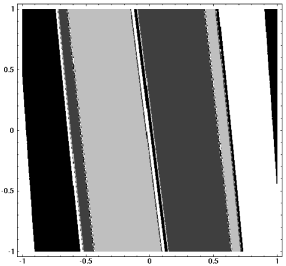
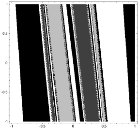
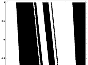
FIG. 2.: Outcomes for null geodesics in two centre geometries with $a=0,\;1$ and $\sqrt{3}$ (arranged from top to bottom).

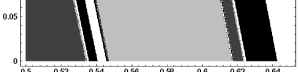
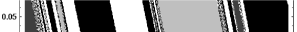
FIG. 3.: Details of Fig. 2

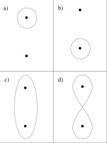
FIG. 4.: Primary unstable orbits.

FIG. 5.: The symbolic dynamics.

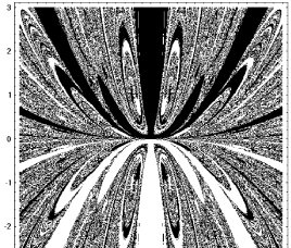
FIG. 6.: Outcomes for massive, uncharged test particles released from rest in the $(a=\sqrt{3})$ two centre geometry.

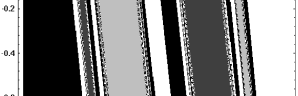
FIG. 7.: Outcome basins for extremal test particles in geometries with $a=0$ and $a=\sqrt{3}$ (arrange top to bottom).

REFERENCES

- [1] C. G. J. Jacobi, 1842 lecture in Vorlesungen uber Dynamik, pp. 189-198, ed. A. Clebsh (1866).
- [2] S. D. Majumdar, Phys. Rev. 72, 390 (1947).
- [3] A. Papapetrou, Proc. R. Irish Acad. A51, 191 (1947).
- [4] J. B. Hartle & S. W. Hawking, Commun. Math. Phys. 26, 87 (1972).
- [5] G. W. Gibbons, Nucl. Phys. B207, 337 (1982); G. W. Gibbons & K. Maeda, Nucl. Phys. B298, 741 (1988); D. Garfinkle, G. Horowitz & Strominger, Phys. Rev. D43, 3140 (1991).
- [6] A. Strominger & C. Vafa, hep-th/9601029 (1996); S. R. Das & S. D. Mathur, hep-th/9601152 (1996).
- [7] S. Chandarasekhar, Proc. R. Soc. London A421, 227 (1989).
- [8] G. Contopoulos, Proc. R. Soc. London A431, 183 (1990); A435, 551 (1991).
- [9] C. P. Dettmann, N. E. Frankel & N. J. Cornish, Phys. Rev. D50, R618 (1994); Fractals, 3, 161 (1995).
- [10] N. J. Cornish & J. J. Levin, The mixmaster universe is chaotic, preprint UM-P-96/33, CfPA-96-TH-10, gr-qc/9605029 (1996).
- [11] A phenomena first suggested by Janna Levin.
- [12] M. Szydlowski, J. Szczȩsny and M. Biesiada, Chaos, Solitons and Fractals 1, 233 (1991); M. Szydlowski and A. Krawiec, Phys. Rev. D47, 5323 (1993); M. Szydlowski, Phys. Lett. A176, 22 (1993); M. Szylowski and J. Szczȩsny, Phys. Rev. D50, 819 (1994); M. Szydlowski J. Math. Phys. 35 (1994); M. Szydlowski Phys. Lett. A201, 19 (1995); M. Szydlowski, M. Heller and W. Sasin, J. Math. Phys. 37, 346 (1996).
- [13] U. Yurtsever, Phys. Rev. D52, 3176 (1995).
- [14] M. Biesiada and S. Rugh, preprint gr-qc/9408030 (1994).
- [15] Y. Sota, S. Suzuki and K. Maeda, Class. Quantum Grav. 13, 1241 (1996); preprint gr-qc/9610065 (1996).
- [16] J. Hadamard J. Math. Pures Appl. 4, 27 (1898).
- [17] C. Robinson, Ergodic Theory Dyn. Syst. 8, 395 (1988).
- [18] V. Benci & F. Giannoni, Duke Math. J. 68, 195 (1992).
- [19] G. W. Gibbons, Phys. Lett. B 308 (1993) 237-239.
- [20] S. W. Hawking & G. F. R. Ellis, The large scale structure of spacetime, (Cambridge University Press, Cambridge, 1973).
- [21] N. J. Cornish, preprint gr-qc/9602054; D. Witt & K. Schleich, preprint gr-qc/9612017 (1996).
- [22] E. Ott, Chaos in dynamical systems, (Cambridge University Press, Cambridge, 1993).
- [23] G. W. Gibbons & C. G. Wells, DAMTP preprint, gr-qc/9310002, (1993).
- [24] A. T. Fomenko Symplectic Geometry, Advanced Studies in Contemporary Mathematics 5, (Gordon and Breach, 1988).