Tachyon field in Loop Quantum Cosmology: inflation and evolution picture

Abstract

Loop quantum cosmology (LQC) predicts a nonsingular evolution of the universe through a bounce in the high energy region. We show that this is always true in tachyon matter LQC. Different from the classical Friedman-Robertson-Walker (FRW) cosmology, the super inflation can appear in the tachyon matter LQC; furthermore, the inflation can be extended to the region where classical inflation stops. Using numerical method, we give an evolution picture of the tachyon field with an exponential potential in the context of LQC. It indicates that the quantum dynamical solutions have the attractive behavior as the classical solutions do. The whole evolution of the tachyon field is that in the distant past, the tachyon field–being in the contracting cosmology–is accelerates to climb up the potential hill with a negative velocity; then at the boundary the tachyon field is bounced into an expanding universe with positive velocity rolling down to the bottom of the potential. In the slow roll limit, we compare the quantum inflation with the classical case in both an analytic and numerical way.

I Introduction

Quantum gravity is expected to rectify the classical general relativity in the regime of high curvature where the classical theory breaks down. Cosmology provides a stage to test this rectification, especially in the region near the big bang singularity. Loop quantum gravity (LQG) is a nonpertubative and background independent approach to quantize gravity lqg . The underlying geometry in LQG is discrete in Planck scale. Loop quantum cosmology (LQC) uses the framework developed in LQG to analyze the universe lqc ; mathematical-structure . In LQC, the spatial geometry is also discrete, and when approaching the Planck scale the universe is described by the difference equation which can go through the big bang point nonsingularly. Above the Planck scale the discreteness of the spatial geometry becomes weak, and the spacetime recovers continuum. However the dynamical equation (effective Hamiltonian constraint) gets modification from LQC both in the gravity and matter secter. This region is known as the semiclassical region in LQC semiclassical . In the semiclassical region, based on the modification from the inverse scale factor operator, many phenomena have been investigated, such as a natural inflation from quantum geometry inflation-geometry , avoidance of a big crunch in closed cosmology avoidance-big-crunch , appearance of a cyclic universe cyclic-universe , and a mass threshold of black hole mass-threshold , etc.

Recent investigation shows that the big bang is replaced by a big bounce by evolving the semiclassical states backwards. And the effective dynamics predicted by the effective Hamiltonian is shown to match very well with the evolution of the semiclassical state bigbang ; effective-theory . In the effective Hamiltonian constraint, the Friedmann equation gets a quadratic density modification for the Hubble rate $H=\dot{a}/a$, $H^{2}\propto\rho\left(1-\rho/\rho_{c}\right)$, which is relevant in the high energy regime bounce . However, this kind of modification is independent of the inverse volume modification. Based on the modified Friedman equation, some interesting results are obtained. For example, it leads to generic bounces when the energy density approaches a critical value $\rho_{c}$ ($\rho_{c}$ is about $0.82$ times the Planck density) bounce ; the scaling solutions of the modified Friedmann equation have a dual relationship with those in Randall-Sundrum cosmology dual ; the future singularity can be avoided with the modified Friedmann equation future .

In cosmology, the tachyon field might be responsible for the cosmological inflation at early epochs and could contribute to some new form of cosmological dark matter at late times Sen1 . In the framework of LQC, based on the inverse volume modification in the matter part, the author of Ref. AAAsen has discussed the properties of the tachyon matter field. It is shown that there exists a super accelerated phase in the semiclassical region, and the solution of the modified Friedmann equation corresponds to the power law solution of the classical equation of the tachyon matter in the classical FRW cosmology. However, as shown in Ref. dual , the quadratic density modification dominates over the inverse volume modification, and the latter can be suitably neglected when the value of the half-integer parameter $j$ (which marked the inverse volume modification) is small. In Ref. Preprration , we discuss the role of $j$ for the effective dynamics, and it is shown that neglecting the inverse volume modification does not affect the behavior of the modified Friedmann equation qualitatively. Therefore, in this paper we shall investigate the behavior of the tachyon matter field in the context of LQC based on the $\rho^{2}$ modification and neglect the inverse volume modification. It is expected that LQC will greatly change the behavior of the tachyon field in the high energy region, especially when the critical density $\rho_{c}$ is approached. We find that, for the tachyon matter cosmology, there exists the superaccelerated phase in the region $\frac{1}{2}\rho_{c}<\rho<\rho_{c}$ as the usual scalar field in LQC dual , and the inflationary e-folding can be increased due to the LQC modification. It is difficult to obtain the exact solutions for the modified Friedman equation and the Hamiltonian equations for the tachyon matter, therefore we analyze the evolution of the tachyon field in LQC by the numerical method. The numerical results show that the evolution of the tachyon matter LQC behaves very differently than in FRW cosmology.

In this paper we only treat the tachyon field as a scalar field with a nonstandard kinetic term, without claiming any identification of the tachyon field with the string tachyon field.

This paper is organized as follows. In Sec. II, we will introduce the tachyon field into the effective theory of LQC and present the state parameter equation in the modified Friedmann equation. Then in Sec. III, we use the numerical method to study the evolution of the tachyon field with an exponential potential in LQC, and the slow roll inflation is also investigated. Finally, Sec. IV is the conclusion.

II Tachyon matter in loop quantum cosmology

In this section, we will first introduce the tachyon field in the FRW cosmology, then the Hamiltonian formulation of the tachyon field can be put in the context of LQC where the dynamics is described by the effective Hamiltonian.

According to Sen Sen1 , in a spatially flat FRW cosmology the Hamiltonian for the tachyon field can be written as

$$H_{\phi}\left(\phi,\Pi_{\phi}\right)=a^{3}\sqrt{V^{2}\left(\phi\right)+a^{-6}\Pi_{\phi}^{2}},$$ (1)

where $\Pi_{\phi}$ is the conjugate momentum for the tachyon field $\phi$, $V\left(\phi\right)$ is the potential term for the tachyon field, and $a$ is the FRW scale factor. Here, we start with the Hamiltonian formulation but not the Lagrangian form, because LQC takes the canonical quantization procedure where the dynamical law is described by the Hamiltonian constraint.

Now the Hamiltonian equations are given by

$$\dot{\phi}=\frac{\partial H_{\phi}}{\partial\Pi_{\phi}}=\frac{a^{-3}\Pi_{\phi}}{\sqrt{V^{2}+a^{-6}\Pi_{\phi}^{2}}},$$ (2)

$$\dot{\Pi}_{\phi}=-\frac{\partial H_{\phi}}{\partial\phi}=-\frac{a^{3}VV^{{}^{\prime}}}{\sqrt{V^{2}+a^{-6}\Pi_{\phi}^{2}}},$$ (3)

where the prime denotes $dV\left(\phi\right)/d\phi$. From Eq. (2), one can also obtain the conjugate momentum as

$$\Pi_{\phi}=\frac{a^{3}V\dot{\phi}}{\sqrt{1-\dot{\phi}^{2}}}$$ (4)

which is just the definition of the conjugate momentum for the tachyon field in the Lagrangian formulation.

Using the Hamiltonian equations, one can get the evolution equation of the tachyon field as

$$\ddot{\phi}=-\left(1-\dot{\phi}^{2}\right)\left(3H\dot{\phi}+\frac{V^{{}^{\prime}}}{V}\right)$$ (5)

where $H=\dot{a}/a$ is the Hubble parameter.

In the Hamiltonian formulation, one cannot identify the matter density and pressure for the tachyon field in the usual way by varying the action of the tachyon field with respect to the spacetime metric. However, one can define the energy density and the pressure as pressure

$$\rho_{\phi}=a^{-3}H_{\phi},\ P_{\phi}=-\frac{1}{3}a^{-2}\frac{\partial H_{\phi}}{\partial a}.$$ (6)

Using Eq. (4), one can find that the expressions of the matter density and pressure obtained from the above definition are the same as those in the Lagrangian formulation:

$$\rho_{\phi}=\frac{V}{\sqrt{1-\stackrel{{\scriptstyle.}}{{\phi}}^{2}}},P_{\phi}=-V\sqrt{1-\stackrel{{\scriptstyle.}}{{\phi}}^{2}}.$$ (7)

Next, we will introduce the tachyon field in the context of LQC, we will focus on the semiclassical region of LQC where the evolution of the universe is described by the effective Hamiltonian constraint and the spacetime recovers the continuum.

LQG is a canonical quantization of gravity. In LQG, the phase space of the classical general relativity is expressed in terms of SU(2) connection $A_{a}^{i}$ and densitized triads $E_{i}^{a}$. In the homogeneous and isotropic cosmology, the symmetry of spacetime reduces the phase space of infinite freedom degrees to finite ones. Thus, in LQC the classical phase space consists of the conjugate variables of the connection $c$ and triad $p$, which satisfy Poisson bracket $\left\{c,p\right\}=\frac{1}{3}\gamma\kappa$, where $\kappa=8\pi G$ ($G$ is the gravitational constant) and $\gamma$ is the Barbero-Immirzi parameter which is fixed to be $\gamma\approx 0.2375$ by the black hole thermodynamics. For the flat model, the new variables have the relations with the metric components of the FRW cosmology as

$$c=\gamma\dot{a},\quad p=a^{2}$$ (8)

where $a$ is the FRW scale factor. In terms of the connection and triad, the classical Hamiltonian constraint is given by mathematical-structure

$$H_{cl}=-\frac{3}{\kappa\gamma^{2}}\sqrt{p}c^{2}+H_{M}.$$ (9)

For quantization in LQC, the elementary variables are the triads and holonomies of connection along an edge which is defined as $h_{i}\left(\mu\right)=\cos\left(\mu c/2\right)+2\sin\left(\mu c/2\right)\tau_{i}$, where $\mu$ is the length of the $i$th edge with respect to the fiducial metric, and $\tau_{i}$ is related to Pauli matrices as $\tau_{i}=-\frac{i}{2}\sigma_{i}$. There is no quantum operator corresponding to the connection $c$, but the holonomies and the triads have well defined quantum operators such that for quantization the Hamiltonian constraint must be reformulated as the elementary variables, i.e., the holonomies and triad. So, the Hamiltonian constraint operator can be obtained by promoting the holonomies and triad to the corresponding operators. The underlying geometry in LQC is discrete, and the quantum Hamiltonian constraint incorporating this discreteness can evolve through the big bang point nonsingularly.

Some long standing questions remain to be systematically answered, such as whether the cosmology can evolve through the classical singular point, etc. The semiclassical state is constructed in bigbang , and evolving the semiclassical state backward in the expanding universe reveals that near the singularity the universe bounces into a contracting branch. It also shows that the quantum feature of the universe can be well described by the effective theory which predicted a quadratic matter density correction for the modified Friedmann equation. For the effective theory, the region is above the Planck scale where the spacetime recovers the continuum, and the dynamical equation takes the usual differential form.

The effective Hamiltonian constraint is given by bigbang ; effective-theory

$$H_{eff}=-\frac{3}{\kappa\gamma^{2}\bar{\mu}^{2}}\sqrt{p}\sin^{2}\left(\bar{\mu}c\right)+H_{M},$$ (10)

where $\bar{\mu}$ is related to the physical area of the square loop over which the holonomies are computed, and the area is $\bar{\mu}^{2}p=\alpha\ell_{Pl}^{2}$ ($\alpha$ is order one and $\ell_{Pl}=\sqrt{G\hbar}$, where $\hbar$ is the reduced Planck constant) fixed by the minimal area in LQG. Here, the matter Hamiltonian $H_{M}$ is expressed by the tachyon field $H_{\phi}$ given by the equation (1). Using the Hamiltonian constraint (10) one can get the Hamiltonian equation

$$\dot{p}=\left\{p,H_{eff}\right\}=-\frac{\gamma\kappa}{3}\frac{\partial H_{eff}}{\partial c}.$$ (11)

Squaring the above equation and substitution of the vanishing Hamiltonian constraint $H_{eff}\approx 0$, the modified Friedmann equation can be obtained as

$$H^{2}=\frac{\kappa}{3}\rho_{\phi}\left(1-\frac{\rho_{\phi}}{\rho_{c}}\right),$$ (12)

where $\rho_{c}=\frac{3}{\kappa\gamma^{2}\bar{\mu}^{2}a^{2}}=\frac{3}{\kappa\gamma^{2}\alpha\ell_{Pl}^{2}}$. Here, the matter density follows the definition in the Eq. (7). As analyzed in bounce , the modified Friedmann equation predicts a nonsingular bounce when the matter density approaches the critical value $\rho_{c}$.

In the context of the effective Hamiltonian, the Hamiltonian equations of the tachyon field behave as its classical ones, so the energy conservative equation is still satisfied as

$$\dot{\rho}_{\phi}+3H\left(\rho_{\phi}+P_{\phi}\right)=0.$$ (13)

Differentiating the modified Friedmann equation with respect to time, then using Eq. (13) above, we get

$$2\dot{H} = -\kappa\left(\rho_{\phi}+P_{\phi}\right)\left(1-\frac{2\rho_{\phi}}{\rho_{c}}\right)$$ (14)

$$= -\kappa\frac{V}{\sqrt{1-\dot{\phi}^{2}}}\left(1-\frac{1}{\rho_{c}}\frac{2V}{\sqrt{1-\dot{\phi}^{2}}}\right).$$

From the above equation we know that when the energy density is in the range: $\frac{1}{2}\rho_{c}<\rho_{\phi}<\rho_{c}$, $\dot{H}$ is always greater than zero. This implies that there exists a superinflation phase for the tachyon matter cosmology. Here, the quantum geometry modification is incorporated, which is different from the inverse volume modification where the superinflation depends on the quantization ambiguity parameter $j$ AAAsen .

As in Ref. bounce , we can analyze the bounce behavior of the tachyon matter cosmology. Whether a bounce or recollapse happens depends on the sign of $\ddot{p}\left|{}_{\dot{p}=0}\right.$. Differentiating the Eq. (11) with respect to the time and using the Hamiltonian equation about $\dot{c}$ given by the Hamiltonian constraint (10), one can get

$$\ddot{a}\left|{}_{\dot{a}=0}\right.=\frac{\kappa}{2}a\left(\rho_{c}-\frac{1}{3}a^{-2}\frac{\partial H_{\phi}}{\partial a}\right)=\frac{\kappa}{2}a\left(\rho_{c}+P_{\phi}\right)$$ (15)

where the second line uses the definition of the pressure. For the tachyon field the state parameter equation is $\omega=\frac{P_{\phi}}{\rho_{\phi}}=-\left(1-\dot{\phi}^{2}\right)$, so the above equation can be rewritten as

$$\ddot{a}\left|{}_{\dot{a}=0}\right.=\frac{\kappa}{2}a\rho_{c}\left(1+\omega\right)=\frac{\kappa}{2}a\rho_{c}\dot{\phi}^{2}\geqslant 0.$$ (16)

Therefore, in the context of LQC for the tachyon matter cosmology, a bounce always exists by which a singularity can be avoided.

Now, we can obtain the modified Raychaudhuri equation as

$$\frac{\ddot{a}}{a} = \dot{H}+H^{2}=-\frac{\kappa}{6}\left\{\rho_{\phi}\left(1-\frac{\rho_{\phi}}{\rho_{c}}\right)\right.$$ (17)

$$\left.+3\left[P_{\phi}\left(1-\frac{\rho_{\phi}}{\rho_{c}}\right)-\frac{\rho_{\phi}^{2}}{\rho_{c}}\right]\right\}.$$

Comparing with the classical Friedmann and Raychaudhuri equation, the effective matter density and pressure can be identified as

$$\rho_{eff}=\rho_{\phi}\left(1-\frac{\rho_{\phi}}{\rho_{c}}\right),$$ (18)

$$P_{eff}=P_{\phi}\left(1-\frac{\rho_{\phi}}{\rho_{c}}\right)-\frac{\rho_{\phi}^{2}}{\rho_{c}},$$ (19)

then the modified Raychaudhuri equation can be rewritten as

$$\frac{\ddot{a}}{a}=-\frac{\kappa}{6}\left(\rho_{eff}+3P_{eff}\right).$$ (20)

One can easily checked that the effective matter density and the pressure still satisfies the conservative equation

$$\dot{\rho}_{eff}+3H\left(\rho_{eff}+P_{eff}\right)=0.$$ (21)

For $\rho_{\phi}\ll\rho_{c}$, one can get $\rho_{eff}\sim\rho_{\phi}$ and $P_{eff}\sim P_{\phi}$, then

$$\frac{\ddot{a}}{a}=-\frac{\kappa}{6}\left(\rho_{\phi}+3P_{\phi}\right).$$

It means that in the case of $\rho_{\phi}\ll\rho_{c}$ the Raychaudhuri equation behave as classically as the modified Friedmann equation and the quantum effect can be neglected.

For $\rho_{\phi}\rightarrow\rho_{c}$ (high energy density region, the critical density $\rho_{c}$ is on the order of Planck density) the modification from the quantum geometry dominates, such that the classical singularity is replace by a bounce. At at the bounce point $\rho_{eff}\sim 0$ and $P_{eff}\sim-\rho_{c}$, so a superinflation happens after the bounce. In the superinflation period, the effective matter density increase with the expansion of the universe until the effective matter density attains the maximum value $\frac{1}{2}\rho_{c}$, then the superinflation phase ends. In the classical tachyon matter cosmology the evolution of the tachyon field can not cross the $\omega=-1$, so the superinflation of tachyon matter in LQC purely comes from the effect of the quantum geometry.

Furthermore, for the modified Raychaudhuri equation, the inflation stops when the right hand side of the Eq. (20) satisfies $\rho_{eff}+3P_{eff}=0$. So at the inflection point, the matter density is

$$\rho_{\phi}=\frac{3\omega+1}{3\omega+4}\rho_{c}.$$ (22)

For the tachyon matter field, $\omega\in\left[-1,0\right]$. If the state parameter $\omega=-\frac{1}{3}$ at the inflection point, then $\rho_{\phi}=0$. This means that for the case of $\omega=-\frac{1}{3}$ the end of the inflation needs matter density $\rho_{\phi}=0$. However, really for tachyon matter field, $\omega=-\frac{1}{3}\Rightarrow$ $\rho_{\phi}=-3P_{\phi}>0$. So, for the tachyon matter field , classically the inflation ends when the state parameter $\omega=-\frac{1}{3}$; however, in the context of LQC, the inflation phase can extend to the region where the classical inflation stops. The effect of the extended inflation phase is only notable when the inflation ends at the high energy region. If the inflation happens at the low energy region (i.e., $\rho_{\phi}\ll\rho_{c}$) where the quantum effect can be neglected, the quantum and classical inflation approaches the same trajectory.

III Evolution of tachyon field with an exponential potential in LQC

III.1 Evolution picture

In this subsection, we will investigate the evolution of the tachyon field in the context of LQC. It is difficult to obtain the analytic solution for the modified Friedmann equation, so we will use numerical method to tackle this issue. In the space of solutions for the tachyon field with an exponential potential, the inflation attractor has been discussed attractor . From the above analysis we know that the inflation of the tachyon field is independent of any initial condition, and it is purely coming from the quantum geometry effect. It is expected that the inflation attractor still can be kept for the effective dynamics. Using the numerical analysis of the evolution of the tachyon field, we find that it is true and different from the classical FRW cosmology. The inflationary attractor appears both in the expanding and contracting cosmology in the context of LQC. In the following, we will discuss these results.

Because of the Hamiltonian constraint, the four dimensional dynamical phase space ($c\left(t\right),p\left(t\right),\phi\left(t\right),\dot{\phi}\left(t\right)$) reduces to three dimensional one. Here, we will show the two dimensional phase portrait consisting of $\phi$ and $\dot{\phi}$. As shown in Ref. bounce , for the evolution of the tachyon matter cosmology the bounce is a critical point which connects the expanding and contracting branches. The cosmology evolving forward at the bounce instant enters the expanding branch. Conversely it is in the contracting branch.

Now, substituting the modified Friedmann Eq. (12) into the conservative Eq. (13), and using the expressions of the energy density and the pressure (7), one can obtain the dynamical equation of the tachyon matter field $\phi$

$$\ddot{\phi} = -\left(1-\dot{\phi}^{2}\right)\frac{V^{{}^{\prime}}}{V}\mp 3\dot{\phi}\left(1-\dot{\phi}^{2}\right)$$ (23)

$$\times\left[\frac{\kappa}{3}\frac{V}{\sqrt{1-\dot{\phi}^{2}}}\left(1-\frac{V}{\rho_{c}\sqrt{1-\dot{\phi}^{2}}}\right)\right]^{1/2},$$

where prime denotes $\frac{d}{d\phi}$. Here, the “$-$” sign describes the expanding branch of the tachyon field, the “$+$” sign expresses the contracting branch. Here the potential for the tachyon field is taken asSen2

$$V\left(\phi\right)=V_{0}\exp\left(-\alpha\phi\right),$$

where $V_{0}$ is positive constant and $\alpha$ is the tachyon mass.

For the tachyon matter cosmology the bounce occurs at the matter density $\rho_{\phi}=\rho_{c}$, i.e.,

$$\frac{V_{0}\exp\left(-\alpha\phi\right)}{\sqrt{1-\dot{\phi}^{2}}}=\rho_{c}.$$ (24)

The critical density constraints the boundary for the evolution of the tachyon field which lies in the band given by the Eq. (24). For the tachyon density, the different values of the constant $V_{0}$ and the mass $\alpha$ only give out the different locations of the boundary in the phase space. The qualitative properties of the evolution can not be changed by the different values of the parameter $V_{0}$ and $\alpha$. In our numerical calculation we take the constant $V_{0}=0.82$ and the mass $\alpha=0.5$. For the boundary $\rho_{\phi}=\rho_{c}$, $\phi$ is in the region $\left[0,\infty\right]$.

Figure 1 shows the expanding branch of the tachyon cosmology. The phase space trajectories obtained from the LQC dynamics are shown as solid lines, and the classical trajectories given by Eq. (5) are shown as dashed lines. Figure 1 indicates that for different values of $\phi$ and $\dot{\phi}$ on the boundary with the rolling of the tachyon field the quantum trajectories approach the same line. This implies that the quantum dynamics do not affect the attractor of the solutions as do the classical solutions analyzed in Ref. attractor . Figure 1 also shows the attractor behaviors of the classical solutions. With the tachyon field rolling down to larger value of $\phi$, the quantum and classical attractors close to each other and merge. Near the boundary, it is in the high energy region where the quantum effect is notable, and the classical trajectories deviate from the quantum ones. The classical trajectories can evolve out of the boundary towards a singularity. However, on the boundary the quantum trajectories are bounced into the contracting cosmology. The complete evolution of the quantum trajectories is shown in the Fig.2.

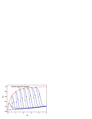
Figure 1: Phase portrait for the expanding branch of tachyonic LQC. The classical trajectories denoted by dash lines are not limmited by the boundary; here we only show the the classical evolution trajectoreis in the inner part of the boundary.

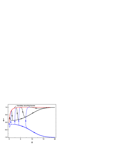
Figure 2: Sketch of the complete evolution of tachyonic LQC. Here, the solid lines and dash lines denote, respectively, the expanding branch and the contracting branch. Also, the bounce occurs on the boundary which connects the two branches.

Figure 2 shows the complete evolution of the tachyon field in LQC. In general, for an inflationary tachyon matter field with an exponential potential, only the first quadrant of the phase space is used, but not the others. In LQC, however, for the phase space of the tachyon field, the first quadrant describes an expanding cosmology with inflation in the high energy region, and the fourth quadrant gives out a contracting cosmology which also has the attractor behavior on the space of solutions. The bounce occurs on the boundary which connects the two branches. Figure 2 tells us that: for the expanding branch, with the evolution of the tachyon field, the evolution velocity $\dot{\phi}$ tends to $1$ and the filed $\phi$ increases to $\infty$; for the contracting branch, with the evolution of the tachyon field to the large value, the evolution velocity $\dot{\phi}$ approaches $-1$. With the increasing field $\phi$, the potential of the tachyon field monotonously decreases and the tachyon field rolls down toward the minimum of the potential. Thus, the whole evolution of the tachyon field can be described as the following: in the distant past, the field, being in the contracting branch, with a negative velocity $-1$ is accelerated climbing up the potential hill; and then the field is bounced into an expanding universe with positive velocity rolling down to the bottom of the potential.

The maximum of the exponential potential is determined by the minimal value of the field $\phi$ not corresponding to the bounce point. In the phase space, the maximum of the potential is at the velocity $\dot{\phi}=0$, where the field $\phi$ takes the minimum value. This can be easily understood, since a negative $\dot{\phi}$ always decreases the value of $\phi$ leading to an increasing exponential potential and conversely a positive velocity decreases the potential. So the maximum potential lies at $\dot{\phi}=0$. Figure 3 shows the rolling of the tachyon field for the potential with the parameter time $t,$ where $t=0$ is set to be the bounce point. In LQC, the tachyon field does not monotonously rolls down to the bottom of the potential as the classical tachyon field dose, but it is driven to climb up the potential hill, and it then rolls down to the minimum of the potential. The sketch of the potential for tachyon field with respect to the evolution time is shown in Fig.3. Furthermore, in LQC, we can say that a negative velocity of the field helps the tachyon field climb up the potential hill and a positive velocity makes the tachyon rolls down to the bottom of the potential.

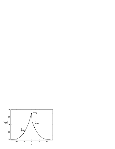
Figure 3: Sketch of the potential for tachyon field with respect to the evolution time. For different quantum trajectory the maximum of the potential is different; here we choose the quantum trajectory for which the field $\phi$ takes $\phi=1.0$ at the boundary to show the potential.

III.2 Slow roll inflation

For the tachyonic cosmology, a successful inflation can be described by the slow roll condition attractor . Figure 1 shows that for the small value of $\dot{\phi}$ the quantum trajectories approach the classical inflationary attractor. So, we can employ the same slow roll condition to analyze the inflationary e-folding for the tachyonic LQC.

In the slow roll limit,

$$\frac{\dot{a}\left(t\right)}{a\left(t\right)}\backsimeq\sqrt{\frac{\kappa}{3}V\left(\phi\right)\left(1-\frac{V\left(\phi\right)}{\rho_{c}}\right)},$$ (25)

and the Hamiltonian Eq.(5) becomes

$$3H\dot{\phi}\backsimeq-\frac{V^{{}^{\prime}}\left(\phi\right)}{V\left(\phi\right)}=\alpha.$$ (26)

On the right-hand side of Eq.(25) the term $\left(1-V\left(\phi\right)/\rho_{c}\right)$ marks the quantum geometry modification. In order to obtain the analytic behavior of tachyonic LQC, we approximately replace the term $\left(1-V\left(\phi\right)/\rho_{c}\right)$ by a constant $\lambda$. Because $0<1-V\left(\phi\right)/\rho_{c}<1$, accordingly $0<\lambda<1$, and $\lambda=1$ corresponds to the classical case without the quantum modification.

Now, Eq.(25) can be written as

$$\frac{\dot{a}\left(t\right)}{a\left(t\right)}\backsimeq\sqrt{\frac{\kappa}{3}\lambda V\left(\phi\right)}.$$ (27)

Substituting Eq.(27) to Eq.(26) and integrating it, the field $\phi$ can be expressed as

$$\phi\left(t\right)=-\frac{2}{\alpha}\ln\left(C-\frac{\alpha^{2}}{6\gamma}t\right),$$ (28)

where $C=\exp\left(-\frac{\alpha}{2}\phi_{i}\right)$ ($\phi_{i}$ denotes the value of $\phi$ at the start of inflation) and $\gamma=\sqrt{\frac{\kappa V_{0}}{3}\lambda}$. Combination of the expression $\phi\left(t\right)$ with Eq.(27) leads to the times of the inflation as attractor

$$\frac{a\left(t_{end}\right)}{a_{i}}=\exp\left[\frac{3}{\alpha^{2}}\left(\lambda\frac{\kappa V_{0}}{3}C^{2}-\frac{\alpha^{2}}{6}\right)\right],$$ (29)

where $a_{i}\left(t_{i}=0\right)$ and $a\left(t_{end}\right)$ respectively denote the values of the scale factor at the start and the end of the inflation.

The above analysis indicates that, for an exponential potential in the slow roll limit, the e-folding number of the tachyonic LQC is smaller than the classical one, i.e.,

$$\left.\frac{a\left(t_{end}\right)}{a_{i}}\right|_{quan,\ \lambda<1}<\left.\frac{a\left(t_{end}\right)}{a_{i}}\right|_{cl,\text{ }\lambda=1}.$$ (30)

Using the evolution Eq.(23) for the tachyon matter LQC, the numerical calculation for the quantum e-folding can be obtained as

$$N_{quan}\left|{}_{\phi_{i}=0.001,\ \dot{\phi}_{i}=0.0316}\right. = \ln\frac{a\left(t_{end}\right)}{a_{i}}=\int_{t_{i}}^{t_{end}}Hdt=\int_{t_{i}}^{t_{end}}\sqrt{\frac{\kappa}{3}\rho_{\phi}\left(1-\frac{\rho_{\phi}}{\rho_{c}}\right)}dt$$

$$= \int_{t_{i}}^{t_{end}}\sqrt{\frac{\kappa}{3}\frac{V_{0}\exp\left(-\alpha\phi\right)}{\sqrt{1-\dot{\phi}^{2}}}\left(1-\frac{V_{0}\exp\left(-\alpha\phi\right)}{\rho_{c}\sqrt{1-\dot{\phi}^{2}}}\right)}dt\simeq 42,$$

where the constant $V_{0}$ and the tachyon mass $\alpha$ take the values as in the above subsection, $\kappa=8\pi G$ ($G=1$ for the nature unit), $\phi_{i}$ and $\dot{\phi}_{i}$ are the initial values for the inflation bounded by the boundary condition. Here, the end time $t_{end}$ of the inflation is determined by the condition $\omega_{eff}:=P_{eff}/\rho_{eff}=-\frac{1}{3}$. Similarly, using the numerical method for the classical inflation the number of the e-folding, we find that

$$N_{cl}\left|{}_{\phi_{i}=0.001,\ \dot{\phi}_{i}=0.0316}\right.=\int_{t_{i}}^{t_{end}}Hdt=\int_{t_{i}}^{t_{end}}\sqrt{\frac{\kappa}{3}\rho_{\phi}}dt\simeq 84,$$

where $\phi_{i}$ and $\dot{\phi}_{i}$ are the initial values for the inflation and they take values on the boundary. It is clear that the numerical calculations shows the result given by the Eq.(30).

A successful inflation needs sixty e-folding. From the Eq.(29), we know that for tachyon matter LQC a sufficient inflation favors a bigger constant $V_{0}$ in the exponential potential or smaller tachyon mass $\alpha$ compared with the values of the parameters used in our numerical calculation. For a small mass $\alpha=0.4$, the numerical calculation shows the number of e-folding of the tachyonic LQC is

$$N_{quan}\left|{}_{\phi_{i}=0.001,\dot{\phi}_{i}=0.0282}\right.=\int_{t_{i}}^{t_{end}}\sqrt{\frac{\kappa}{3}\rho_{\phi}\left(1-\frac{\rho_{\phi}}{\rho_{c}}\right)}dt\simeq 65$$

where $V_{0}$ takes the value as in the above.

Furthermore, it is also interesting to analyze the slow roll inflation for other choice of the potential. For example, for an inverse square potential padman one can compare the quantum inflation with the classical case.

IV Conclusion

In this paper we discuss the tachyon field in the context of LQC. LQC essentially incorporates the discrete quantum geometry effect. So, in the high energy region (approaching the critical density $\rho_{c}$), LQC greatly modifies the classical FRW cosmology and predicts a nonsingular bounce at the critical density $\rho_{\phi}=\rho_{c}$. We show that this is always true in the tachyon matter LQC. For the tachyon matter LQC, a superinflation can appear in the region $\frac{1}{2}\rho_{c}<\rho_{\phi}<\rho_{c}$. This superinflation phase purely comes from the quantum effect. In FRW cosmology, the state parameter equation $\omega$ of the tachyon field belongs to $\left[-1,0\right]$, so the superinflation phase is lacking. In order to closely examine the modification to the classical FRW equation, it is helpful to identify the effective density $\rho_{eff\text{ }}$ and the pressure $P_{eff}$ based on the modified Friedmann equation. We find that the effective density and the pressure still satisfy the energy conservative equation. Furthermore, the modified Raychaudhuri equation described by the effective density and the pressure implies that the inflation phase can be extended to the region where the classical inflation stops. This effect is notable only when the inflation ends in a high energy region.

The next issue what we have investigated is the evolution of the tachyon field with an exponential potential. Using the numerical method, we have found that, as in FRW cosmology, the solutions of the tachyon field still keep the attractor behavior in LQC, and we have found that with the evolution of tachyon field all the quantum and classical trajectories approach each other and merge. At the high energy region (approaching the critical density), the classical trajectories deviate from the quantum ones. Evolving the tachyon field backward on the boundary, the tachyon matter cosmology is bounced into an contracting branch. In the phase space the first quadrant describes the expanding branch, and the fourth quadrant expresses the contracting branch. So, the evolution picture of the tachyon field in LQC is this: in the distant past, the field-being in the contracting branch with a negative velocity $-1$-is accelerated to climb up the potential hill; then the field is bounced into an expanding universe with positive velocity rolling down to the bottom of the potential. What is more, the maximum potential can be attained when the rolling velocity of the tachyon field is equal to zero. In the slow roll limit, the number of quantum e-folds is smaller than it is in the classical case. For tachyonic LQC a sufficient inflation favors a bigger constant $V_{0}$ in the exponential potential or small tachyon mass $\alpha$.

We analyze the evolution of tachyon field with the exponential potential in the context of LQC, and obviously, any other choice of potential can be investigated via the same way. In fact, one may also study cosmological consequences of tachyon matter field in the context of the string theory. But as Kofman and Linde emphasized in Ref. problem , we face some problems with tachyon field, such as the difficulty to obtain the inflation and the failure of reheating, etc. LQC can naturally predict an inflation phase which is independent of the choice of a particular potential and extend the physical phase space of the tachyon field to the fourth quadrant. We hope that this work can shed light on some of the problems of understanding the tachyon field.

- (1) C. Rovelli, Quantum Gravity (Cambridge University Press, Cambridge, 2004); T. Thiemann, Introduction to Modern Canonical Quantum General Relativity, gr-qc/0110034.
- (2) M. Bojowald, Living Rev. Relativity 8, 11 (2005). (See: http://relativity.livingreviews.org/Articles/lrr-2005-11/index.html)
- (3) A. Ashtekar, M. Bojowald and J. Lewandowski, Adv. Theor. Math. Phys. 7, 233-68 (2003).
- (4) P. Singh, K. Vandersloot, Phys. Rev. D 72, 084004 (2005).
- (5) M. Bojowald, Phys. Rev. Lett. 89, 261301 (2002).
- (6) P. Singh, A. Toporensky, Phys. Rev. D 69, 104008 (2004).
- (7) M. Bojowald, R. Maartens and P. Singh, Phys. Rev. D 70, 083517 (2004).
- (8) M. Bojowald, R. Goswami, R. Maartens, and P. Singh, Phys. Rev. Lett. 95, 091302 (2005).
- (9) A. Ashtekar, T. Pawlowski, and P. Singh, Phys. Rev. D 73, 124038 (2006); A. Ashtekar, T. Pawlowski, and P. Singh, Phys. Rev. D 74, 084003 (2006).
- (10) V. Taveras, IGPG report, 2006.
- (11) P. Singh, K. Vandersloot, G. V. Vereshchagin, Phys. Rev. D 74, 043510 (2006).
- (12) P. Singh, Phys. Rev. D. 73, 063508 (2006).
- (13) M. Sami, P. Singh and S. Tsujikawa, Phys. Rev. D 74, 043514 (2006).
- (14) A. Sen, J. High Energy Phys. 04, 048(2002); 07, 065(2002).
- (15) A. A. Sen, Phys. Rev. D. 74, 043501(2006).
- (16) Hua-Hui Xiong and Jian-Yang Zhu, gr-qc/0702002.
- (17) G.M. Hossain, Classical Quantum Gravity 22, 2653 (2005).
- (18) M. Sami, P. Chingangbam and T. Qureshi, Phys. Rev. D. 66, 043530 (2002); Z. K. Guo, Y. S. Piao and R. G. Cai, Phys. Rev. D. 68, 043508(2003).
- (19) A. Sen, Mod. Phys. Lett. A 17, 1797 (2002).
- (20) T. Padmanabhan, Phys. Rev. D 66, 021301 (2002).
- (21) L. Kofman, A. Linde, J. High Energy Phys. 07, 004 (2002).