Effect of the Inverse Volume Modification in Loop Quantum Cosmology

Abstract

It is known that in loop quantum cosmology (LQC) the universe avoids the singularity by a bounce when the matter density approaches the critical density $\rho_{c}$ (the order of Planck density). After incorporating the inverse volume modifications both in the gravitational and matter part in the improved framework of LQC, we find that the inverse volume modification can decrease the bouncing energy scale, and the presence of nonsingular bounce is generic. For the backward evolution in the expanding branch, in terms of different initial states the evolution trajectories classify into two classes. One class with larger initial energy density leads to the occurrence of bounce in the region $a>a_{ch}$ where $a_{ch}$ marks the different inverse volume modification region. The other class with smaller initial energy density evolves back into the region $a<a_{ch}$. In this region, both the energy density for the scalar field and the bouncing energy scale decrease with the backward evolution. However, in the deep modification region, because of the inverse volume modification the scalar field is frozen, such that the bounce is present when the bouncing energy scale decreases to be equal to the energy density of the scalar field. Using numerical method, we show the evolution picture for the second class bounce.

I Introduction

In cosmology, an outstanding problem is the big bang singularity which is expected to be solved by quantum gravity. Loop quantum cosmology (LQC) uses the framework developed from loop quantum gravity (LQG) LQG to deal with the issues in cosmology lqc ; mathematical-structure . As a ramification of LQG, LQC inherits the nonperturbative and background independent feature of LQG. In LQC, the underlying geometry is discrete as in LQG, and the universe evolution is described by the difference equation which can go through the singularity nonsingularly singularity-free .

The central technical issue in LQC is to quantize the Hamiltonian constraint which generates the dynamical law. The classical Hamiltonian constraint consists of the basic variables, i.e., the SU(2) valued holonomies and the densitized triads. Conventionally, on quantization of the Hamiltonian constraint, the SU(2) valued holonomies in the gravitational part traces over the $J=1/2$ fundamental representation, while in the matter part the SU(2) representation can be freely specified to define the inverse volume resulting in the quantization ambiguity known as inverse scale factor modification. Based on such quantum Hamiltonian constraint, the effective dynamics can be obtained by some approximation. By use of the effective dynamics one can investigate some phenomena in the semiclassical region, where the spacetime recovers the continuum and the difference equation is replaced by a differential equation Date ; semiclassical-state . A number of results, such as a natural inflation from quantum geometry inflation-geometry ; Xiong-Zhu , avoidance of a big crunch in closed cosmology avoidance-bigcrunch , an oscillating universe with suitable initial condition for inflation oscillating-universe , appearance of a cyclic universe cyclic-universe and a mass threshold of black hole mass-threshold , etc, are interesting and remarkable.

As shown in Ref. inverse-volume , the quantization ambiguity also can appear in the gravitational part. Using arbitrary $J$ representation for the holonomies, the Hamiltonian constraint operator is constructed in Ref. inverse-volume . It shows that in the semiclassical region the gravitational Hamiltonian gets modification similar to the inverse volume modification in the matter part. This is because that, in the classical Hamiltonian constraint, both the gravitational part and matter part contain inverse volume terms, and, for quantization, promoting the inverse volume into Poisson bracket between the volume and the holonomies leads to the same quantization ambiguity quantization-ambiguity . Therefore, as a phenomenal investigation, in the semiclassical region the inverse volume modification appearing in the gravitational part should also be included.

Recently, the semiclassical state is constructed in Refs. bigbang ; improved-dynamics , and the most important result is that, by evolving the semiclassical state backwards in the high energy density regime, the expanding universe bounces into a contracting branch, so that the singularity can be avoided. An effective Hamiltonian constraint incorporating the discrete quantum geometry can well describe the evolution of the semiclassical state improved-dynamics ; preprint . This constraint predicts a quadratic density correction in the modified Friedmann equation for the Hubble rate $H=\dot{a}/a$, $H^{2}\varpropto\rho(1-\rho/\rho_{c})$. The modified Friedmann equation implies a bounce when the matter density approaches the critical density $\rho_{c}$ ($\rho_{c}$ is about $0.82$ times the Planck density). Using the modified Friedmann equation, some interesting results are obtained: a bounce can happen avoiding of the singularity when the energy density approaches the critical value $\rho_{c}$ nonsingular-bounce ; the scaling solutions of the modified Friedmann equation have dual relationship with those in Randall-Sundrum cosmology dual ; the future singularity can be avoided by the modified Friedmann equation future-singularity . However, in these works the inverse volume modification is neglected both in the gravitational part and the matter part, and for the gravitational part the holonomies are valued only on the $J=1/2$ fundamental representation. Furthermore, from the viewpoint of lattice model, a large spin $J$ means a longer range interaction between lattices which appear as background structures lattice , and the inverse volume modification also could contribute to the seed of structure formation structure . The effect of the inverse volume modifications to the effective dynamics is still unclear for the improved framework. Some further questions still need to be answered: What is the effect of the inverse volume modification in the gravitational part of the effective dynamics? What is its effect on the matter part? We shall look into these questions in the framework of the effective Hamiltonian.

In Ref. improved-dynamics , the improved Hamiltonian constraint operator is introduced. The minimal area gap can be better exploited by the improved Hamiltonian to realize the physical idea, i.e., in the flat model a bouncing universe is present purely because of the discrete quantum geometry. In this paper, we work in the improved framework to analyze the effect of the inverse volume modification both in the gravitational part and matter part of the effective dynamics. We find that the inverse volume modification in the gravity sector raised by a bigger quantization ambiguity parameter $J$ could decrease the energy scale at the bounce point. And, whether a bounce really happens or not depends on whether the matter density at the high energy region attains the bouncing energy scale. The inverse volume modification greatly changes the matter density below the scale $a_{*}$. With the backward evolution in an expanding universe, in the region $a<a_{ch}$ the scalar field is frozen such that a nonsingular bounce is present. Our numerical results show the genericness of bounce in LQC.

This article is organized as follows. In Sec. II, we give a brief review over the Hamiltonian constraint and the modified Friedmann equation. Then in Sec. III, the effect of the inverse volume modification in universe evolution is analyzed in detail. Section IV contains our numerical results, displaying the evolution picture of the nonsingular bouncing universe. Finally, the concluding remarks are made in Sec. V.

II Hamiltonian constraint and modified Friedmann equation

II.1 Classical and quantum Hamiltonian constraint

LQC is a canonical quantization of cosmology model mimicing the quantizing procedures as in the full theory. Imposing on the homogeneous and isotropic symmetry in LQC, the classical phase space is reduced to two degrees of freedom consisting of the conjugate connection $c$ and triad $p$. The Poisson bracket between the conjugate variables satisfies $\left\{c,p\right\}=\frac{1}{3}\gamma\kappa$, where $\kappa=8\pi G$ ($G$ is the gravitational constant), and $\gamma$ is the dimensionless Barbero-Immirzi parameter whose value, $\gamma\approx 0.2375$, set by the black hole entropy calculation. For the flat model, the usual Friedman-Robertson-Walker (FRW) metric expression can be identified with the relation given by

$$c=\gamma\dot{a},\ \left|p\right|=a^{2},$$ (1)

where $a$ is the FRW scale factor, and the absolute value of $p$ denotes the two orientations of the triad. Here, we only take the positive orientation. In terms of the connection and triad, the classical Hamiltonian constraint is given by mathematical-structure

$$H=H_{G}+H_{M},\ H_{G}=-\frac{3}{\kappa\gamma^{2}}\text{sgn}(p)\sqrt{\left|p\right|}c^{2}.$$ (2)

On quantization in LQC, there is no operator directly corresponding to the connection $c$. Instead, the elementary variables are the triad $p$ and the holonomies $h_{i}(\mu)$ defined as the connection $c$ along an edge, i.e., $h_{i}(\mu)=e^{\mu c\tau_{i}}$, where $\mu$ is the length of the $i$th edge, and $\tau_{i}$ is a basis in the Lie algebra su(2) satisfying $\left[\tau_{i},\tau_{j}\right]=\varepsilon_{ijk}\tau^{k}$. As in LQG, the holonomies and triads have well-defined operators. So, the Hamiltonian constraint given by Eq. (2) must be reformulated in terms of the holonomies and the triads. The gravitational part of the Hamiltonian constraint $H_{G}$ in the full theory can be written as mathematical-structure

$$H_{G}=-\frac{1}{\kappa\gamma^{2}}\int d^{3}x\varepsilon_{k}^{ij}\frac{E_{i}^{a}E_{j}^{b}}{\sqrt{\left|\det E\right|}}F_{ab}^{k},$$ (3)

where $F_{ab}^{k}$ is the curvature component of the connection.

The strategies for quantization are: first, to reformulate the Hamiltonian constraint by the holonomies and triads, and then, to promote these elementary variables to the corresponding operators. The term $E_{i}^{a}E_{j}^{b}/\sqrt{\left|\det E\right|}$ contains the inverse volume, and on quantization the inverse volume is promoted to the commutator of the holonomy and volume, resulting in the quantization ambiguity labeled by the spin representation $J$. For the $J=1/2$ fundamental representation, the quantum operator for the gravitational part is given by

$$\widehat{H}_{G} = \frac{i}{4\pi\kappa\ell_{p}^{2}\gamma^{3}\overline{\mu}^{3}}\sum_{ijk}\varepsilon^{ijk}Tr\left(\hat{h}_{i}\hat{h}_{j}\hat{h}_{i}^{-1}\hat{h}_{j}^{-1}\hat{h}_{k}\left[\hat{h}_{k}^{-1},\hat{V}\right]\right)$$ (4)

$$= \frac{6i}{\pi\kappa\ell_{p}^{2}\gamma^{3}\bar{\mu}^{3}}\sin^{2}\left(\frac{\bar{\mu}c}{2}\right)\cos^{2}\left(\frac{\bar{\mu}c}{2}\right)$$

$$\times\left(\sin\left(\frac{\bar{\mu}c}{2}\right)\hat{V}\cos\left(\frac{\bar{\mu}c}{2}\right)-\cos\left(\frac{\bar{\mu}c}{2}\right)\hat{V}\sin\left(\frac{\bar{\mu}c}{2}\right)\right),$$

where $\ell_{p}^{2}=G\hbar$ ($\hbar$ is the reduced Planck constant) and the volume operator $\hat{V}=\hat{p}^{3/2}$. In Eq. (4) the holonomies are valued along the edges of the square loop whose area is fixed by the minimal eigenvalue of area operator in LQG. The physical area of the square loop is $\bar{\mu}^{2}p=\alpha\ell_{p}^{2}$, where $\alpha$ is order one. The area of the loop fixed by the minimal area of LQG shows the discrete feature of quantum geometry. We shall see that this point essentially captures the effect of quantum geometry making the effective dynamics very different from the classical case in the high energy regime. As for the arbitrary $J$ representation, the gravitational Hamiltonian operator can be constructed as done in Ref. inverse-volume . One only replaces the fixed parameter $\mu_{0}$ with $\bar{\mu}$. As shown in Ref. improved-dynamics , replacing $\mu_{0}$ with $\bar{\mu}$ is a key step to realize the improved Hamiltonian constraint. After obtaining the gravitational Hamiltonian constraint operator for arbitrary $J$ representation, it is useful to extract the effective theory which is expected to capture the key feature of the Hamiltonian constraint operator in the semiclassical region. Next, we will show the inverse volume modification raised by the quantization ambiguity parameter $J$ in the effective theory.

II.2 Effective Hamiltonian constraint

It is shown in Ref. improved-dynamics that the quantum evolution determined by the quantum Hamiltonian constraint is nonsingular in big bang point. By evolving the semiclassical states backwards, the universe evolution indicates that the big bang is replaced by a bounce when the matter density approaches the critical value $\rho_{c}$. This feature can be well described by the effective Hamiltonian constraint in the region which is above the Planck scale and where spacetime recovers the continuum. The effective Hamiltonian can be obtained by the WKB approximation Date ; semiclassical-state or by a systematic way low-energy . Here, the effective Hamiltonian for the arbitrary $J$ representation is given by dual ; low-energy ; vandersloot

$$H_{eff}=-\frac{3}{\kappa\gamma^{2}\bar{\mu}^{2}}S_{J}\left(p\right)\sin^{2}\left(\bar{\mu}c\right)+H_{M},$$ (5)

where $S_{J}\left(p\right)$ encodes the inverse volume modification for the gravitational part and is given by

$$S_{J}\left(p\right)=\sqrt{p}S\left(\frac{p}{p_{J}}\right),$$ (6)

and

$$S\left(q\right) = \frac{4}{\sqrt{q}}\left\{\frac{1}{10}\left[\left(q+1\right)^{\frac{5}{2}}+sgn\left(q-1\right)\left|q-1\right|^{\frac{5}{2}}\right]\right.$$

$$\left.-\frac{1}{35}\left[\left(q+1\right)^{\frac{7}{2}}-\left|q-1\right|^{\frac{7}{2}}\right]\right\},$$

where $p_{J}=\frac{8\pi\gamma J\bar{\mu}}{3}\ell_{P}^{2}$ mark the modification region, below which (i.e., $q<1$) the modification is dramatic, and above which the effect of the inverse volume modification can be neglected with $S\left(q\right)\approx 1$.

II.3 Modified Friedmann equation

II.3.1 Small $J$ modification

One can assume that $J$ is small, then $S_{J}\left(p\right)\approx\sqrt{p}$ and the effective Hamiltonian becomes

$$H_{eff}=-\frac{3}{\kappa\gamma^{2}\bar{\mu}^{2}}\sqrt{p}\sin^{2}\left(\bar{\mu}c\right)+H_{M}.$$ (8)

Such an effective Hamiltonian presents a singularity-free bouncing universe with the modified Friedmann equation improved-dynamics ; nonsingular-bounce

$$H^{2}=\frac{\kappa}{3}\rho\left(1-\frac{\rho}{\rho_{c}}\right),$$ (9)

where $H$ is the Hubble parameter, the critical density $\rho_{c}=3/\kappa\gamma^{2}\bar{\mu}^{2}a^{2}=3/\kappa\gamma^{2}\alpha\ell_{p}^{2}$ and the matter density $\rho=H_{M}/p^{3/2}$. Based on the effective equation (9) some interesting issues have been discussed nonsingular-bounce ; dual ; future-singularity .

II.3.2 Large $J$ modification

Now, we discuss the large $J$ modification to the effective dynamics. By the effective Hamiltonian constraint given by Eq. (5), the Hamiltonian equation can be obtained as

$$\dot{p}=\left\{p,H_{eff}\right\}=-\frac{\gamma\kappa}{3}\frac{\partial H_{eff}}{\partial c}.$$ (10)

The Hamiltonian equation (10) gives out

$$a\dot{a}=\frac{1}{\gamma\bar{\mu}}S_{J}\left(a^{2}\right)\sin\left(\bar{\mu}c\right)\cos\left(\bar{\mu}c\right).$$ (11)

Squaring the above equation and then making use of the Hamiltonian constraint $H_{eff}\approx 0$, the modified Friedmann equation incorporating the inverse volume modification can be obtained as

$$H^{2}=\frac{\kappa}{3}\rho\left(S\left(q\right)-\frac{\rho}{\rho_{c}}\right),$$ (12)

where $q\equiv p/p_{J}=\left(a/a_{g*}\right)^{2}$.

III Effect of the inverse volume modification in universe evolution

III.1 Modification in the gravitational sector

The modified Friedmann Eq. (12) gives out the evolution of the universe. In the early time of the universe, if the matter density $\rho=S\left(q\right)\rho_{c}$, then there exists a turn-around. At the turn-around, a bounce or a collapse happens depending on the sign of the second derivative of the triad with time. For the effective theory one can analyze the bounce behavior of the universe as discussed in Ref. nonsingular-bounce . From the Hamiltonian Eq. (10) and $\dot{c}=\left\{c,H_{eff}\right\}$, one can get

$$\ddot{p}\left|{}_{\dot{p}=0}\right. = \kappa S_{J}^{2}(p)\left[\frac{2}{3}\left(1+\frac{d\ln S_{J}\left(p\right)}{d\ln p}\right)\rho_{c}-\frac{1}{S\left(q\right)}\left(\frac{2}{3}\frac{1}{\sqrt{p}}\frac{\partial H_{M}}{\partial p}\right)\right]$$ (13)

$$= \kappa S_{J}^{2}(p)\left[\frac{2}{3}\left(1+\frac{d\ln S_{J}\left(p\right)}{d\ln p}\right)\rho_{c}+\frac{1}{S\left(q\right)}P\right],$$

where the second line uses the definition of the pressure $P\equiv\frac{2}{3}\frac{1}{\sqrt{p}}\frac{\partial H_{M}}{\partial p}$ as in Ref. pressure-definition . For a constant state parameter equation, i.e., $P=\omega\rho$, the Eq. (13) can be written as

$$\ddot{p}\left|{}_{\dot{p}=0}\right.=\kappa S_{J}^{2}(p)\rho_{c}\left[\frac{2}{3}\left(1+\frac{d\ln S_{J}\left(p\right)}{d\ln p}\right)+\omega\right].$$ (14)

For $p<p_{J}$, the function $d\ln S_{J}\left(p\right)/d\ln p$ monotonically decreases, and when $a\ll a_{*}=\sqrt{p_{J}}$, $\ddot{p}\left|{}_{\dot{p}=0}\right.\rightarrow\kappa S_{J}^{2}(p)\rho_{c}\left(\frac{4}{3}+\omega\right)$; $a\rightarrow a_{*}$, $\ddot{p}\left|{}_{\dot{p}=0}\right.\rightarrow\kappa p_{J}\rho_{c}\left(1.05+\omega\right)$. Therefore, one can obtain that the recollapse requires $\omega<-1$, which classically violates the null energy condition and implies an expanding universe with increasing energy density. This exotic matter behaves like phantom field. In the next section, we shall explicitly give out the expression of the effective state parameter equation $\omega_{eff}$; it will show that the presence of a turn-around always leads to a bouncing universe. So, for the universe with quantum modification, the state parameter equation satisfies $\omega>-1$.

In order to better understand the effect of the inverse volume modification on the modified Friedmann, we shall distinguish the two basic scales: One is the bounce scale $a_{bounce}$, which is determined by the condition $\rho\left(a\right)=S\left(q\right)\rho_{c}$, and whose explicit value is related with the mater content (in the next section we will deal with the related issue). The other one is the inverse volume modification scale $a_{*}=\sqrt{p_{J}}=\sqrt{8\pi\gamma J\bar{\mu}/3}\ell_{P}=\left(8\pi\alpha^{1/2}\gamma/3\right)^{1/3}J^{1/3}\ell_{P}$ ($\bar{\mu}$ is replaced by the fixed area relation $\bar{\mu}^{2}a^{2}=\alpha\ell_{P}^{2}$), whose magnitude depends on the parameter $J$. We know that $a_{bounce}$ is the minimal scale for the evolution of the universe. If the inverse volume modification scale $a_{*}<a_{bounce}$, the effect of the inverse volume modification should be neglected because in this range the inverse volume modification tends to its classical form $S_{J}\left(p\right)=\sqrt{p}$. However, for a large enough $J$, such that $a_{bounce}<a<a_{*}$, then the inverse volume modification becomes notable in LQC.

From the above analysis, we know that for the bouncing universe the matter density at the bouncing energy scale is $\rho_{bounce}=S\left(q\right)\rho_{c}$. In the region $a_{bounce}<a<a_{*}$, the function $S\left(q\right)$ monotonically increases and $S\left(q\right)<1$. For $a_{bounce}\ll a_{*}$, $S\left(q\right)\approx\frac{6}{5}\frac{a}{a_{*}}\ll 1$. Therefore, we can conclude that for LQC the inverse volume modification in the gravitational part reduce the matter density at the bounce point.

In this subsection, we have analyzed the effect of the inverse volume modification to the bouncing universe. However, for LQC, whether a bounce happens or not depends on the content of the matter field. In the next section, we will show the effect of the inverse volume modification in the matter sector on the evolution of LQC.

III.2 Modification in the matter sector

In this section, we focus on the inverse volume modification in the matter sector for the modified Friedmann equation. In earlier literatures, the SU(2) representation for the matter part is labeled by a half integer which can be freely specified independent of the $J$ representation in the gravitational part. As argued in Ref. inverse-volume , it is more natural to take the same representation for them. Therefore, for a massive scalar field with self-interaction potential $V\left(\phi\right)$, the Hamiltonian $H_{M}$ is given by inflation-geometry

$$H_{M}=\frac{1}{2}d_{J}\left(a\right)p_{\phi}^{2}+a^{3}V\left(\phi\right),$$ (15)

where $p_{\phi}$ is the conjugate momentum for the scalar field $\phi$, and $d_{J}\left(a\right)$ is the eigenvalue of the inverse volume operator $\hat{a}^{-3}$ which can be approximately described as

$$d_{J}\left(a\right)=D\left(\frac{a^{2}}{a_{*}^{2}}\right)a^{-3}.$$ (16)

In which, the modification region is still marked by the scale $a_{*}=\left(8\pi\alpha^{1/2}\gamma/3\right)^{1/3}J^{1/3}\ell_{P}$, and the function $D\left(a^{2}/a_{*}^{2}\right)$ respects the inverse volume modification and has the form

$$D\left(q\right) = \left(\frac{8}{77}\right)^{6}q^{\frac{3}{2}}\left\{7\left[\left(q+1\right)^{\frac{11}{4}}-\left|q-1\right|^{\frac{11}{4}}\right]\right.$$ (17)

$$-\left.11q\left[\left(q+1\right)^{\frac{7}{4}}-sgn\left(q-1\right)\left|q-1\right|^{\frac{7}{4}}\right]\right\}^{6}.$$

Above the scale $a_{*}$, $D\left(q\right)\simeq 1$, so the inverse volume modification can be neglected. While at $q\ll 1$, $D\left(a^{2}/a_{*}^{2}\right)\approx\left(12/7\right)^{6}\left(a/a_{*}\right)^{15}$.

Now, the modified Friedmann equation becomes

$$H^{2}=\frac{\kappa}{3}\rho\left[S\left(a^{2}/a_{*}^{2}\right)-\frac{\rho}{\rho_{c}}\right]$$ (18)

where the matter density $\rho=H_{M}/p^{3/2}$ which receives the inverse volume modification.

From the Hamiltonian equation $\dot{\phi}=\left\{\phi,H_{M}\right\}$, one can get

$$p_{\phi}=d_{J}^{-1}\left(a\right)\dot{\phi}.$$ (19)

It leads to the matter density

$$\rho=\frac{1}{2}D^{-1}\dot{\phi}^{2}+V\left(\phi\right).$$ (20)

Differentiating Eq.(19) and substituting it into another Hamiltonian equation $\dot{p}_{\phi}=\left\{p_{\phi},H_{M}\right\}$, the modified Klein-Gordon equation can be obtained as

$$\ddot{\phi}=-3H\left(1-\frac{1}{3}\frac{d\ln D}{d\ln a}\right)\dot{\phi}-DV^{{}^{\prime}}\left(\phi\right),$$ (21)

where prime denotes $\frac{d}{d\phi}$. Then the time derivative of the matter density is

$$\dot{\rho}=-3HD^{-1}\dot{\phi}^{2}\left(1-\frac{1}{6}\frac{d\ln D}{d\ln a}\right),$$ (22)

where $d\ln D/d\ln a$ is a monotonically decreasing function in the region $a<a_{*}$. So, there exists a characteristic scale $a_{ch}\approx 0.91a_{*}$ determined by $d\ln D/d\ln a=6$, and the mater density attains the maximal value. Classically, with the expansion of the universe, the matter density decreases. However, in the region of $a<a_{ch}$, the matter density increases; above this region the matter density starts to decrease and enters the regime where the quadratic density modification dominates and the effect of the inverse volume modification can be neglected. In the following, we will discuss the possible evolution of LQC in different regions.

First, it is useful to identify the effective matter density and pressure. From Eq. (18), the modified Raychoudhuri equation is written as

$$\frac{\ddot{a}}{a} = \dot{H}+H^{2}$$ (23)

$$= -\frac{\kappa}{6}\left\{-2\rho\left(S-\frac{\rho}{\rho_{c}}\right)-\frac{1}{H}\left(\dot{\rho}S+\rho\dot{S}-\frac{2\rho\dot{\rho}}{\rho_{c}}\right)\right\}.$$

Then the effective energy density and pressure can be defined as

$$\rho_{eff}=\rho\left(S-\frac{\rho}{\rho_{c}}\right),$$ (24)

$$P_{eff}=-\rho\left(S-\frac{\rho}{\rho_{c}}\right)+\frac{1}{3H}\left(\dot{\rho}S+\rho\dot{S}-\frac{2\rho\dot{\rho}}{\rho_{c}}\right).$$ (25)

They satisfy the conservative equation

$$\dot{\rho}_{eff}+3H\left(\rho_{eff}+P_{eff}\right)=0.$$ (26)

Substituting Eq. (22) into the expression of $P_{eff}$, the effective state parameter equation is

$$\omega_{eff}=\frac{P_{eff}}{\rho_{eff}}=-1+\frac{2\dot{\phi}^{2}\left(1-\frac{1}{6}\frac{d\ln D}{d\ln a}\right)}{\dot{\phi}^{2}+2DV\left(\phi\right)}\frac{S-\frac{2\rho}{\rho_{c}}}{S-\frac{\rho}{\rho_{c}}}-\frac{2}{3}q\frac{\frac{dS}{dq}}{S-\frac{\rho}{\rho_{c}}},$$ (27)

where the function $dS/dq$ monotonically decreases in the region $a<a_{*}$, and asymptotically vanishes beyond this region. From the effective parameter equation we know that both the inverse volume modification and the quadratic density correction can contribute to the inflation of the universe.

In LQC, the evolution trajectory is determined by the dynamical initial condition dynamical-condition . So, we evolve the universe at large scale $a\gg$ $a_{*}$ backwards in the expanding universe where the matter density $\rho\ll\rho_{c}$ and the quantum modifications can be neglected. With the backward evolution, the matter density increases in the region $a>a_{ch}$. If the matter density satisfies $\rho\geqslant S\left(a_{ch}^{2}/a_{*}^{2}\right)\rho_{c}$, then $\rho_{eff}=0$ leads to a bouncing universe which is caused purely by the quadratic density modification. This situation is similar to the case of $a_{bounce}\geqslant a_{*}$, where the inverse volume modification can be neglected. If the mater density $\rho<S\left(a_{ch}^{2}/a_{*}^{2}\right)\rho_{c}$, the universe evolves back to the deep inverse volume modification region $a<a_{ch}$. In the region $a<a_{ch}$, from Eqs. (II.2) and (22) we know that both the matter density $\rho$ and the bouncing energy scale $S(q)\rho_{c}$ decrease with the backward evolution. If the bouncing energy scale $S(q)\rho_{c}$ decreases faster than the matter density, then there is no bounce; the universe will evolve towards the big bang point where the effective theory is invalid and the quantum difference equation takes over the evolution of the universe. Another possible way is that the mater density decreases more slowly than the bouncing energy scale, until $\rho=S(q)\rho_{c}$, where a bounce happens and the universe is bounced into a contracting branch. We would like to point out that the actual evolution way favors the latter. It is because that, with the backward evolution, the density decrease. However, for the density $\rho=\frac{1}{2}D^{-1}\dot{\phi}^{2}+V\left(\phi\right)$, in the small volume, the term $D^{-1}\varpropto\left(a/a_{*}\right)^{15}$ is far larger than one. This needs the velocity $\dot{\phi}$ to be extremely small, such that the field is frozen. So, the kinetic term can be neglected, and the potential dominates. With the decreasing scale $a$, the field is frozen, until the bouncing energy scale $S\left(a^{2}/a_{*}^{2}\right)\rho_{c}$ decreases to be equal to the potential $V\left(\phi\right)$. At that point, a bounce happens. In what follows, using the numerical way, we will show the evolution of the universe.

IV Genericness of bounce shown in numerical results

In the inverse volume modification region, a negative scalar potential can lead to a bouncing universe only when the condition $\rho=0$ is satisfiedcyclic-universe ; early-universe . This is also true for the modified Friedmann equation presented in this paper. From the modified Raychoudhuri Eq. (23), it is easily seen that in the region $a<a_{ch}$ the vanishing density implies a bounce. Such bounce purely comes from the inverse volume modification. The reason is that the inverse volume modification in this region makes

$$\frac{\ddot{a}}{a}\left|{}_{\dot{a}=0}\right.=-\frac{\kappa}{2}D^{-1}\dot{\phi}^{2}\left(1-\frac{1}{6}\frac{d\ln D}{d\ln a}\right)S\left(q\right)>0,$$

which implies a bounce. In the following, we will show the evolution trajectory of LQC with a positive potential.

Using the modified Friedmann Eq. (18) and the Klein-Gordon Eq. (21), we can obtain the dynamical law for the universe with a massive scalar field with the potential $V\left(\phi\right)=m^{2}\phi^{2}/2$. Here, for the numerical calculation we take the mass $m=0.2$. From the above discussion we know that these trajectories can be divided into two classes: the ones with higher energy density can be bounced into an contracting branch in the region $a>a_{ch}$, and the others with lower energy density $\rho<S\left(a_{ch}^{2}/a_{*}^{2}\right)\rho_{c}\approx 0.94\rho_{c}$ evolve back to the deep modification region $a<a_{ch}$. In this paper, we are only concerned about the latter. For the backward evolution, we take the initial state marked by the energy density $\rho_{in}$ at the scale $a_{ch}$. Our numerical results show that the presence of a bounce is generic for theses trajectories with the initial state $\rho_{in}$ in the region $\left(0.001\sim 1\right)S\left(a_{ch}^{2}/a_{*}^{2}\right)\rho_{c}$. Below this region, we think that it is not suitable to take the energy density far below the Planck density as the initial state in the quantum modification region. The initial state can be written as

$$\rho_{in}\left(a_{ch}\right) = \frac{1}{2}D^{-1}\left(a_{ch}^{2}/a_{*}^{2}\right)\dot{\phi}^{2}+\frac{1}{2}m^{2}\phi^{2}$$ (28)

$$= \lambda S\left(a_{ch}^{2}/a_{*}^{2}\right)\rho_{c},$$

where $\lambda$ denotes the initial state with different initial energy. From Eqs. (18) and (21) we know that under the rescaled transformation $a\rightarrow a/a_{*}$ the dynamical equations do not change and do not depend on the scale $a$ explicitly. So, under this rescaling we can take an arbitrary value of $J$ to show the evolution trajectories. For other choices of $J$, the evolution trajectories are the same as the chosen one. Here, we take $J=1000$ to show the evolution picture.

Figure 1 shows the presence of bounce for $\lambda=0.5$. For different initial values of $\phi$, the bouncing scale is different. With larger value of $\left|\phi\right|$, the bouncing scale is larger. The contrary is that with larger value of $\left|\dot{\phi}\right|$, the bounce happens at deeper region. This can be regarded as that, for the backward evolution, a larger kinetic term takes longer distance to be frozen. At the bouncing point, the field is frozen at some fixed value of $\phi$. Figure 2 shows that with the backward evolution the scalar field is frozen and then bounced into a contracting branch. For other choices of $\lambda$, the bouncing behavior is similar as presented in Figs. 1 and 2. The difference is that with smaller value of $\lambda$ the bounce happens at deeper region.

Furthermore, in the inverse volume modification region the scalar field can be pushed to climb up the potential hill. As a result, this can set the initial condition for a classical inflation CMB-spectrum . To achieve 60 e-folds of inflation for a quadratic potential $V=m^{2}\phi^{2}/2$ , the field must be displaced by at least $3M_{Pl}$ from the minimum of its potential at the onset of inflation. For the case of $\lambda=0.5$ presented in the above, this means that for a successful inflation the bounce should happen at bigger scale for larger value of $\left|\phi_{in}\right|$ shown in Fig. 1.

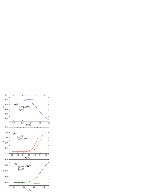
Figure 1: The evolution of the scale factor is shown for a scalar field with potential $V\left(\phi\right)=m^{2}\phi^{2}/2$ for different initial states distinguished by different initial values of $\phi_{in}$(these initial states are constrained by the fixed initial energy density $\rho_{in}=0.5S\left(a_{ch}^{2}/a_{*}^{2}\right)\rho_{c}\approx 0.74\rho_{c}$ at the scale $a_{ch}$, and $\dot{\phi}_{in}$ is determined by Eq.28). The solid lines denote the expanding branch, and the dashed lines show the contracting branch. In the region $a<a_{ch}\approx 0.91a_{*}$, the backward evolution shows that for bigger initial value of $\left|\phi_{in}\right|$ the bounce happens at bigger scale.

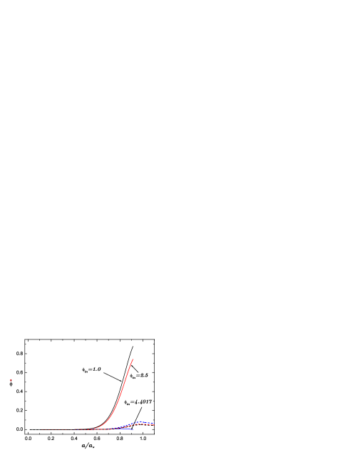
Figure 2: The sketch shows that near the bouncing scale the scalar field is frozen such that the kinetic term vanishes and the potential dominates. Here, the solid lines and the dashed lines denote, respectively, the expanding branch and the contracting branch. The initial states take values as in Fig. 1 constrained by the fixed initial energy density $\rho_{in}=0.5S\left(a_{ch}^{2}/a_{*}^{2}\right)\rho_{c}\approx 0.74\rho_{c}$.

V Conclusion

In this paper, we mainly discuss the effect of the inverse volume modifications on the effective dynamics, which implies a nonsingular bounce for the evolution of the universe when the matter density approaches the high energy region. This is a nontrivial result compared with the bouncing mechanism in the fundamental $J=1/2$ representation improved-dynamics ; nonsingular-bounce . Because until now there is still lack of a complete quantization for large $J$ representation in the improved framework, we expect that the evolution picture presented in this paper will be given by a complete quantum theory as in improved-dynamics . Furthermore, we argue that the genericness of bounce in the high spin representation is not accidental: the presence of bounce is a consequence of the fact that LQC essentially incorporates two quantum effects, i.e., the inverse volume modifications and the quadratic density modification raised by the minimal area gap, and the two quantum effects jointly induce the occurrence of bounce. For the inverse volume modification, the modification region is marked by the scale $a_{*}$, below which the modifications are notable and above which the modifications become weak. The inverse volume modification in the gravity sector decreases the bouncing energy scale in the region $a_{bounce}<a<a_{g*}$ (neglecting the inverse volume modification the bouncing energy scale is equal to the critical density $\rho_{c}$ ). And, the inverse volume modification in the matter sector changes the classical behavior of density. Below the scale $a_{ch}\approx 0.91a_{*}$ the time derivative of the matter density is positive, implying that, with the backward evolution of an expanding universe, the matter density decreases. So, in the region $a<a_{ch}$ the presence of bounce depends on the relative decreasing rate between the matter density and the bouncing energy scale. However, in the deep quantum modification region the scalar field is frozen. So the kinetic term can be neglected, and the matter density is dominated by the potential. Therefore, the matter density is almost frozen at a fixed value. With the backward evolution, a bounce happens until the bouncing energy scale decreases to be equal to the potential. Our numerical results shown in Figs. 1 and 2 provide a illustration of the evolution pictures. For different initial values of the matter density the bouncing scale is different.

In earlier literatures, the SU(2) representation for the gravitational Hamiltonian is taken to be the fundamental representation, but for the matter Hamiltonian the representation is freely specified. If one does so, then in this paper the modified Friedmann equation becomes $H^{2}=\kappa\rho\left(1-\rho/\rho_{c}\right)/3$, where $\rho=\frac{1}{2}D^{-1}\dot{\phi}^{2}+V\left(\phi\right)$ receives the inverse volume modification. For the backward evolution in the expanding branch, if the matter density increases to be equal to the critical density $\rho_{c}$ in the region $a>a_{ch}$, a bounce happens. If the universe evolves back through the scale $a_{ch}$, the matter density starts to decrease, so a bounce will never be present for the universe with a positive potential. This is a distinct difference between the two views of the inverse volume modification. Moreover, the inverse volume modification can leave indirect imprint on the CMB spectrumCMB-spectrum . We expect the further research could put constraint for the value of $J$ based on the prediction for observations.

In this paper we analyze the effect of the inverse volume modifications on the improved LQC, and we show that the presence of nonsingular bounce is generic.

- (1) C. Rovelli, Quantum Gravity (Cambridge University Press, Cambridge, 2004); T. Thiemann, “Introduction to Modern Canonical Quantum General Relativity”, (CUP, Cambridge, to be published).
- (2) M. Bojowald, Liv. Rev. Rel. 8, 11(2005).
- (3) A. Ashtekar, M. Bojowald and Lewandowski, Adv. Theor. Math. Phys. 7, 233-68 (2003).
- (4) M. Bojowald, Phys. Rev. Lett. 86, 5227 (2001).
- (5) K. Banerjee, G. Date, Classical Quantum Gravity 22, 2017 (2005).
- (6) P. Singh, K. Vandersloot, Phys. Rev. D 72, 084004 (2005).
- (7) M. Bojowald, Phys. Rev. Lett. 89, 261301 (2002).
- (8) Hua-Hui Xiong and Jian-Yang Zhu, Phys. Rev. D 75, 084023 (2007)
- (9) P. Singh, A. Toporensky, Phys. Rev. D 69, 104008 (2004).
- (10) J. E. Lidsey, D. J. Mulryne, N. J. Nunes, and R. Tavakol, Phys. Rev. D 70, 063521 (2004); D. J. Mulryne, N. J. Nunes, R. Tavakol, and J. E. Lidsey, Int. J. Mod. Phys. A 20, 2347 (2005).
- (11) M. Bojowald, R. Maartens and P. Singh, Phys. Rev. D 70, 083517 (2004).
- (12) M. Bojowald, R. Goswami, R. Maartens, and P. Singh, Phys. Rev. Lett. 95, 091302 (2005).
- (13) K. Vandersloot, Phys. Rev. D 71, 103506 (2005).
- (14) M. Bojowald, Classical Quantum Gravity 19, 5113 (2002).
- (15) A. Ashtekar, T. Pawlowski, and P. Singh, Phys. Rev. D 73, 124038 (2006).
- (16) A. Ashtekar, T. Pawlowski, and P. Singh, Phys. Rev. D 74, 084003 (2006).
- (17) V. Taveras, IGPG preprint (2006).
- (18) P. Singh, K. Vandersloot and G.V. Vereshchagin, Phys. Rev. D 74, 043510 (2006).
- (19) P. Singh, Phys. Rev. D. 73, 063508 (2006).
- (20) M. Bojowald, Gen. Relativ. Gravit. 38, 1771 (2006).
- (21) M. Bojowald, Phys. Rev. Lett. 98, 031301 (2007).
- (22) J. Willis, Ph.D. thesis, The Pennsylvania State University, (2004).
- (23) K. Vandersloot, Ph.D. thesis, The Pennsylvania State University, (2006).
- (24) M. Sami, P. Singh and S. Tsujikawa, Phys. Rev. D 74, 043514 (2006).
- (25) G.M. Hossain, Classical Quantum Gravity 22, 2653 (2005).
- (26) M. Bojowald, Phys. Rev. Lett. 87, 121301 (2001).
- (27) J. E. Lidsey, J. Cosmol. Astropart. Phys. 12, 007 (2004).
- (28) S. Tsujikawa, P. Singh and R. Maartens, Classical Quantum Gravity 21, 5767 (2004).