Statefinder diagnosis in a non-flat universe and the holographic model of dark energy

Abstract:

In this paper, we study the holographic dark energy model in non-flat universe from the statefinder viewpoint. We plot the evolutionary trajectories of the holographic dark energy model for different values of the parameter $c$ as well as for different contributions of spatial curvature, in the statefinder parameter-planes. The statefinder diagrams characterize the properties of the holographic dark energy and show the discrimination between this scenario and other dark energy models. As we show, the contributions of the spatial curvature in the model can be diagnosed out explicitly by the statefinder diagrams. Furthermore, we also investigate the holographic dark energy model in the $w-w^{\prime}$ plane, which can provide us with a useful dynamical diagnosis complement to the statefinder geometrical diagnosis.

Nowadays it is strongly believed that the universe is experiencing an accelerated expansion. Recent observations from type Ia supernovae (SNIa) [1] in associated with large scale structure (LSS) [2] and cosmic microwave background (CMB) anisotropies [3] have provided main evidence for this cosmic acceleration. In order to explain why the cosmic acceleration happens, many theories have been proposed. Although theories of trying to modify Einstein equations constitute a big part of these attempts, the mainstream explanation for this problem, however, is known as theories of dark energy. It is the most accepted idea that a mysterious dominant component, dark energy, with negative pressure, leads to this cosmic acceleration, though its nature and cosmological origin still remain enigmatic at present.

The combined analysis of cosmological observations suggests that the universe consists of about $70\%$ dark energy, $30\%$ dust matter (cold dark matter plus baryons), and negligible radiation. Although the nature and origin of dark energy are unknown, we still can propose some candidates to describe it. The most obvious theoretical candidate of dark energy is the cosmological constant $\lambda$ (or vacuum energy) [4, 5] which has the equation of state $w=-1$. However, as is well known, there are two difficulties arise from the cosmological constant scenario, namely the two famous cosmological constant problems — the “fine-tuning” problem and the “cosmic coincidence” problem [6]. The fine-tuning problem asks why the vacuum energy density today is so small compared to typical particle scales. The vacuum energy density is of order $10^{-47}{\rm GeV}^{4}$, which appears to require the introduction of a new mass scale 14 or so orders of magnitude smaller than the electroweak scale. The second difficulty, the cosmic coincidence problem, says: Since the energy densities of vacuum energy and dark matter scale so differently during the expansion history of the universe, why are they nearly equal today? To get this coincidence, it appears that their ratio must be set to a specific, infinitesimal value in the very early universe.

Theorists have made lots of efforts to try to resolve the cosmological constant problem, but all these efforts were turned out to be unsuccessful. However, there remain other candidates to explaining dark energy. An alternative proposal for dark energy is the dynamical dark energy scenario. The cosmological constant puzzles may be better interpreted by assuming that the vacuum energy is canceled to exactly zero by some unknown mechanism and introducing a dark energy component with a dynamically variable equation of state. The dynamical dark energy proposal is often realized by some scalar field mechanism which suggests that the energy form with negative pressure is provided by a scalar field evolving down a proper potential. So far, a large class of scalar-field dark energy models have been studied, including quintessence [7], $K$-essence [8], tachyon [9], phantom [10], ghost condensate [11, 12] and quintom [13], and so forth. But we should note that the mainstream viewpoint regards the scalar field dark energy models as an effective description of an underlying theory of dark energy. In addition, other proposals on dark energy include interacting dark energy models [14], braneworld models [15], and Chaplygin gas models [16], etc.. One should realize, nevertheless, that almost these models are settled at the phenomenological level, lacking theoretical root.

In recent years, many string theorists have devoted to understand and shed light on the cosmological constant or dark energy within the string framework. The famous Kachru-Kallosh-Linde-Trivedi (KKLT) model [17] is a typical example, which tries to construct metastable de Sitter vacua in the light of type IIB string theory. Furthermore, string landscape idea [18] has been proposed for shedding light on the cosmological constant problem based upon the anthropic principle and multiverse speculation. Another way of endeavoring to probe the nature of dark energy within the fundamental theory framework originates from some considerations of the features of the quantum gravity theory. It is generally believed by theorists that we can not entirely understand the nature of dark energy before a complete theory of quantum gravity is established [19]. However, although we are lacking a quantum gravity theory today, we still can make some attempts to probe the nature of dark energy according to some principles of quantum gravity. The holographic dark energy model is just an appropriate example, which is constructed in the light of the holographic principle of quantum gravity theory. That is to say, the holographic dark energy model possesses some significant features of an underlying theory of dark energy.

The distinctive feature of the cosmological constant or vacuum energy is that its equation of state is always exactly equal to $-1$. However, when considering the requirement of the holographic principle originating from the quantum gravity speculation, the vacuum energy will acquire dynamically property. As we speculate, the dark energy problem may be in essence a problem belongs to quantum gravity [19]. In the classical gravity theory, one can always introduce a cosmological constant to make the dark energy density be an arbitrary value. However, a complete theory of quantum gravity should be capable of making the properties of dark energy, such as the energy density and the equation of state, be determined definitely and uniquely. Currently, an interesting attempt for probing the nature of dark energy within the framework of quantum gravity is the so-called “holographic dark energy” proposal [20, 21, 22, 23]. It is well known that the holographic principle is an important result of the recent researches for exploring the quantum gravity (or string theory) [24]. This principle is enlightened by investigations of the quantum property of black holes. Roughly speaking, in a quantum gravity system, the conventional local quantum field theory will break down. The reason is rather simple: For a quantum gravity system, the conventional local quantum field theory contains too many degrees of freedom, and such many degrees of freedom will lead to the formation of black hole so as to break the effectiveness of the quantum field theory.

For an effective field theory in a box of size $L$, with UV cut-off $\Lambda$ the entropy $S$ scales extensively, $S\sim L^{3}\Lambda^{3}$. However, the peculiar thermodynamics of black hole [25] has led Bekenstein to postulate that the maximum entropy in a box of volume $L^{3}$ behaves nonextensively, growing only as the area of the box, i.e. there is a so-called Bekenstein entropy bound, $S\leq S_{BH}\equiv\pi M_{P}^{2}L^{2}$. This nonextensive scaling suggests that quantum field theory breaks down in large volume. To reconcile this breakdown with the success of local quantum field theory in describing observed particle phenomenology, Cohen et al. [20] proposed a more restrictive bound – the energy bound. They pointed out that in quantum field theory a short distance (UV) cut-off is related to a long distance (IR) cut-off due to the limit set by forming a black hole. In other words, if the quantum zero-point energy density $\rho_{\Lambda}$ is relevant to a UV cut-off $\Lambda$, the total energy of the whole system with size $L$ should not exceed the mass of a black hole of the same size, thus we have $L^{3}\rho_{\Lambda}\leq LM_{P}^{2}$. This means that the maximum entropy is in order of $S_{BH}^{3/4}$. When we take the whole universe into account, the vacuum energy related to this holographic principle [24] is viewed as dark energy, usually dubbed holographic dark energy. The largest IR cut-off $L$ is chosen by saturating the inequality so that we get the holographic dark energy density

$$\rho_{\Lambda}=3c^{2}M_{P}^{2}L^{-2}~{},$$ (1)

where $c$ is a numerical constant, and $M_{P}\equiv 1/\sqrt{8\pi G}$ is the reduced Planck mass. Many authors have devoted to developed the idea of the holographic dark energy. It has been demonstrated that it seems most likely that the IR cutoff is relevant to the future event horizon

$$R_{\rm h}(a)=a\int_{t}^{\infty}{dt^{\prime}\over a(t^{\prime})}=a\int_{a}^{\infty}{da^{\prime}\over Ha^{\prime 2}}~{}.$$ (2)

Such a holographic dark energy looks reasonable, since it may provide simultaneously natural solutions to both dark energy problems as demonstrated in Ref.[23]. The holographic dark energy model has been tested and constrained by various astronomical observations [26, 27, 28]. Furthermore, the holographic dark energy model has been extended to include the spatial curvature contribution, i.e. the holographic dark energy model in non-flat space [29]. We focus in this paper on the holographic dark energy in a non-flat universe. For other extensive studies, see e.g. [30].

On the other hand, since more and more dark energy models have been constructed for interpreting or describing the cosmic acceleration, the problem of discriminating between the various contenders is becoming emergent. In order to be capable of differentiating between those competing cosmological scenarios involving dark energy, a sensitive and robust diagnosis for dark energy models is a must. In addition, for some geometrical models arising from modifications to the gravitational sector of the theory, the equation of state no longer plays the role of a fundamental physical quantity, so it would be very useful if we could supplement it with a diagnosis which could unambiguously probe the properties of all classes of dark energy models. For this purpose a diagnostic proposal that makes use of parameter pair $\{r,s\}$, the so-called “statefinder”, was introduced by Sahni et al. [31]. The statefinder probes the expansion dynamics of the universe through higher derivatives of the expansion factor $\stackrel{{\scriptstyle...}}{{a}}$ and is a natural companion to the deceleration parameter $q$ which depends upon $\ddot{a}$. The statefinder is a “geometrical” diagnosis in the sense that it depends upon the expansion factor and hence upon the metric describing space-time.

In this paper we apply the statefinder diagnosis to the holographic dark energy model in the non-flat universe. The statefinder can also be used to diagnose different cases of the model, including various model parameters and different spatial curvature contributions. Analysis of the observational data provides constraints on the holographic dark energy model. In [26, 27], it has been shown that regarding the observational data including type Ia supernovae, cosmic microwave background, baryon acoustic oscillation, and the X-ray gas mass fraction of galaxy clusters, the holographic dark energy in flat universe behaves like a quintom-type dark energy. Moreover, in [32], it has been shown that when including the spatial curvature contribution, the closed universe and quintom-type dark energy are marginally favored, in the light of SNIa and CMB data. We use the statefinder to diagnose these different cases, and the result shows that the information of the spatial curvature can be precisely diagnosed in the statefinder planes.

Consider now the homogenous and isotropic universe described by the Friedmann-Robertson-Walker (FRW) metric

$$ds^{2}=-dt^{2}+a^{2}(t)(\frac{dr^{2}}{1-kr^{2}}+r^{2}d\Omega^{2}),$$ (3)

where $k$ denotes the curvature of the space with $k=0$, 1 and $-1$ corresponding to flat, closed and open universes, respectively. The IR cutoff of the universe in the holographic model $L$ is defined as

$$L=a(t)r,$$ (4)

where $r$ is relevant to the future event horizon of the universe. Given the fact that

$$\int_{0}^{r_{1}}{dr\over\sqrt{1-kr^{2}}} = \frac{1}{\sqrt{|k|}}{\rm sinn}^{-1}(\sqrt{|k|}\,r_{1})$$ (8)

$$= \left\{\begin{array}[]{ll}\sin^{-1}(\sqrt{|k|}\,r_{1})/\sqrt{|k|},&k=1,\\ r_{1},&k=0,\\ \sinh^{-1}(\sqrt{|k|}\,r_{1})/\sqrt{|k|},&k=-1,\end{array}\right.$$

one can easily derive

$$L=\frac{a(t){\rm sinn}[\sqrt{|k|}\,R_{h}(t)/a(t)]}{\sqrt{|k|}},$$ (9)

where $R_{\rm h}$ is the future event horizon given by (2). With normal pressureless matter and holographic dark energy as sources, the Friedmann equations take the form

$$H^{2}=\frac{8\pi G}{3}\rho-\frac{k}{a^{2}},$$ (10)

$$\frac{\ddot{a}}{a}=-\frac{4\pi G}{3}(\rho+3P),$$

where $\rho$ is the total energy density, $\rho=\rho_{\rm m}+\rho_{\Lambda}$, and $P=w\rho_{\Lambda}$ is the pressure of the dark energy component since we know that the normal dust matter is pressureless. Define the density parameters as usual

$$\Omega_{\rm m}=\frac{\rho_{\rm m}}{\rho_{\rm cr}}=\frac{\Omega_{\rm m0}H^{2}_{0}}{H^{2}a^{3}},\hskip 14.22636pt\Omega_{\Lambda}=\frac{\rho_{\Lambda}}{\rho_{\rm cr}}=\frac{c^{2}}{L^{2}H^{2}},\hskip 14.22636pt\Omega_{k}=\frac{k}{a^{2}H^{2}}=\frac{\Omega_{k0}H^{2}_{0}}{a^{2}H^{2}},$$ (11)

then we can rewrite the first Friedmann equation as

$$\Omega_{\rm m}+\Omega_{\rm\Lambda}=1+\Omega_{k}.$$ (12)

Since we have

$$\frac{\Omega_{k}}{\Omega_{\rm m}}=a\frac{\Omega_{k0}}{\Omega_{\rm m0}}=a\gamma,$$ (13)

where $\gamma=\Omega_{k0}/\Omega_{\rm m0}$, we get $\Omega_{k}=\Omega_{\rm m}a\gamma$ and

$$\Omega_{\rm m}=\frac{1-\Omega_{\Lambda}}{1-a\gamma}.$$ (14)

Hence, from the above equation, we get

$$\frac{1}{aH}=\frac{1}{H_{0}}\sqrt{\frac{a(1-\Omega_{\Lambda})}{\Omega_{\rm m0}(1-a\gamma)}}.$$ (15)

Combining Eqs. (9) and (15), and using the definition of $\Omega_{\Lambda}$, we obtain

$$\sqrt{|k|}\frac{R_{h}}{a} = {\rm sinn}^{-1}\left[c\sqrt{|\gamma|}\sqrt{\frac{a(1-\Omega_{\Lambda})}{\Omega_{\Lambda}(1-a\gamma)}}\,\right]$$ (16)

$$= {\rm sinn}^{-1}(c\sqrt{|\Omega_{k}|/\Omega_{\Lambda}}).$$

From the above relationships, the differential equation describing the evolutionary behavior of the holographic dark energy can be derived [29, 32]

$$(1+z){d\Omega_{\Lambda}\over dz}=-{2\over c}\Omega_{\Lambda}^{3/2}(1-\Omega_{\Lambda})\sqrt{1-{c^{2}\gamma(1-\Omega_{\Lambda})\over\Omega_{\Lambda}(1+z-\gamma)}}-(1+z){\Omega_{\Lambda}(1-\Omega_{\Lambda})\over 1+z-\gamma},$$ (17)

where $z=(1/a)-1$ is the red-shift parameter of the universe. This equation completely describes the dynamical evolution of the holographic dark energy, and it can be solved numerically. From the energy conservation equation of the dark energy, the equation of state of dark energy can be given [32]

$$w = -1-\frac{1}{3}\frac{d\ln\rho_{\Lambda}}{d\ln a}$$ (18)

$$= -\frac{1}{3}\left[1+\frac{2}{c}\sqrt{\Omega_{\Lambda}}{\rm cosn}(\sqrt{|k|}\,R_{h}/a)\right]$$

$$= -\frac{1}{3}\left[1+\frac{2}{c}\sqrt{\Omega_{\Lambda}-c^{2}\Omega_{k}}\right],$$

where

$$\frac{1}{\sqrt{|k|}}{\rm cosn}(\sqrt{|k|}x)=\left\{\begin{array}[]{ll}\cos(x),&k=1,\\ 1,&k=0,\\ \cosh(x),&k=-1.\end{array}\right.$$ (19)

The holographic dark energy model has been tested and constrained by various astronomical observations, in both flat and non-flat cases. These observational data include type Ia supernovae, cosmic microwave background, baryon acoustic oscillation, and the X-ray gas mass fraction of galaxy clusters. According to the analysis of the observational data for the holographic dark energy model, we find that generally $c<1$, and the holographic dark energy thus behaves like a quintom-type dark energy. When including the spatial curvature contribution, the fitting result shows that the closed universe is marginally favored. Here we summarized the main constraint results as follows:

1. For flat universe, using only the SNIa data to constrain the holographic dark energy model, we get the fit results: $c=0.21^{+0.41}_{-0.12}$, $\Omega_{\rm m0}=0.47^{+0.06}_{-0.15}$, with the minimal chi-square corresponding to the best fit $\chi^{2}_{\rm min}=173.44$ [26]. In this fitting, The SNIa data used are 157 “gold” data listed in Riess et al. [33] including 14 high redshift data from the Hubble Space Telescope (HST)/Great Observatories Origins Deep Survey (GOODS) program and previous data. Furthermore, when combining the information from SNIa [33], CMB [3] and LSS [34], the fitting for the holographic dark energy model gives the parameter constraints in 1 $\sigma$: $c=0.81^{+0.23}_{-0.16}$, $\Omega_{\rm m0}=0.28\pm 0.03$, with $\chi_{\rm min}^{2}=176.67$ [26]. In this joint analysis, the SNIa data are still the 157 “gold” data [33], the CMB information comes from the measured value of the CMB shift parameter $R$ given by [3] $R\equiv\Omega_{\rm m0}^{1/2}\int_{0}^{z_{\rm CMB}}dz^{\prime}/E(z^{\prime})=1.716\pm 0.062$, where $z_{\rm CMB}=1089$ is the redshift of recombination and $E(z)\equiv H(z)/H_{0}$, and the LSS information is provided by the baryon acoustic oscillation (BAO) measurement [34] $A\equiv\Omega_{\rm m0}^{1/2}E(z_{\rm BAO})^{-1/3}[(1/z_{\rm BAO})\int_{0}^{z_{\rm BAO}}dz^{\prime}/E(z^{\prime})]^{2/3}=0.469\pm 0.017$, where $z_{\rm BAO}=0.35$.

2. Also for the flat case, the X-ray gas mass fraction of rich clusters, as a function of redshift, has also been used to constrain the holographic dark energy model [27]. The $f_{\rm gas}$ values are provided by Chandra observational data, the X-ray gas mass fraction of 26 rich clusters, released by Allen et al. [35]. The main results, i.e. the 1 $\sigma$ fit values for $c$ and $\Omega_{\rm m0}$ are: $c=0.61^{+0.45}_{-0.21}$ and $\Omega_{\rm m0}=0.24^{+0.06}_{-0.05}$, with the best-fit chi-square $\chi_{\rm min}^{2}=25.00$ [27].

3. For the non-flat universe, the authors of [32] used the data coming from the SNIa and CMB to constrain the holographic dark energy model, and got the 1 $\sigma$ fit results: $c=0.84^{+0.16}_{-0.03}$, $\Omega_{\rm m0}=0.29^{+0.06}_{-0.08}$, and $\Omega_{k0}=0.02\pm 0.10$, with the best-fit chi-square $\chi_{\rm min}^{2}=176.12$. Also, in this analysis, the SNIa data come from the 157 “gold” data in Riess et al. [33], and the CMB information still comes from the measured value of the CMB shift parameter $R$ [3].

Now we switch to discussing the statefinder diagnosis of the holographic dark energy model. For characterizing the expansion history of the universe, one defines the geometric parameters $H=\dot{a}/a$ and $q=-\ddot{a}/aH^{2}$, namely the Hubble parameter and the deceleration parameter. It is clear that $\dot{a}>0$ means the universe is undergoing an expansion and $\ddot{a}>0$ means the universe is experiencing an accelerated expansion. From the cosmic acceleration, $q<0$, one infers that there may exist dark energy with negative equation of state, $w<-1/3$ and likely $w\sim-1$, but it is hard to deduce the information of the dynamical property of $w$ from the value of $q$. In order to extract the information of the dynamical evolution of $w$, it seems that we need the higher time derivative of the scale factor, ${\stackrel{{\scriptstyle...}}{{a}}}$. Another motivation for proposing the statefinder parameters comes from the merit that they can provide with a diagnosis which could unambiguously probe the properties of all classes of dark energy models including the cosmological models without dark energy describing the cosmic acceleration. Though at present we can not extract sufficiently accurate information of $\ddot{a}$ and ${\stackrel{{\scriptstyle...}}{{a}}}$ from the observational data, we can expect, however, the high-precision observations of next decade may be capable of doing this. The statefinder parameters can be used to diagnose the evolutionary behaviors of various cosmological models, and discriminate them from each other. In what follows, we shall exam the holographic dark energy model in non-flat universe using the statefinder diagnosis.

Generically, the statefinder pair $\{r,s\}$ is defined as follows [36]

$$r\equiv\frac{\stackrel{{\scriptstyle...}}{{a}}}{aH^{3}},~{}~{}~{}~{}~{}s\equiv\frac{r-\Omega_{\rm tot}}{3(q-\Omega_{\rm tot}/2)}.$$ (20)

Here $\Omega_{\rm tot}$ is the total energy density, $\Omega_{\rm tot}=\Omega_{\rm m}+\Omega_{\Lambda}=1+\Omega_{k}$. Note that the parameter $r$ is also called cosmic jerk. Thus the set of quantities describing the geometry is extended to include $\{H,q,r,s\}$. Trajectories in the $s-r$ plane corresponding to different cosmological models exhibit qualitatively different behaviors. The spatially flat $\Lambda$CDM (cosmological constant $\lambda$ with cold dark matter) scenario corresponds to a fixed point in the diagram

$$\{s,r\}\bigg{|}_{\rm flat-\Lambda CDM}=\{0,1\}~{}.$$ (21)

Departure of a given dark energy model from this fixed point provides a good way of establishing the “distance” of this model from spatially flat $\Lambda$CDM [31]. As demonstrated in Refs. [36, 37, 38, 39, 40, 41, 42, 43, 44, 45, 46, 47, 48] the statefinder can successfully differentiate between a wide variety of dark energy models including the cosmological constant, quintessence, phantom, quintom, the Chaplygin gas, braneworld models and interacting dark energy models. We can clearly identify the “distance” from a given dark energy model to the flat-$\Lambda$CDM scenatio by using the $r(s)$ evolution diagram. The current location of the parameters $s$ and $r$ in these diagrams can be calculated in models. The current values of $s$ and $r$ are evidently valuable since we expect that they can be extracted from data coming from SNAP (SuperNovae Acceleration Probe) type experiments. Therefore, the statefinder diagnosis combined with future SNAP observations may possibly be used to discriminate between different dark energy models. It is notable that in the non-flat universe the $\Lambda$CDM model no longer corresponds a fixed point in the statefinder plane, it exhibits an evolutionary trajectory

$$\{s,r\}\bigg{|}_{\rm nonflat-\Lambda CDM}=\{0,\Omega_{\rm tot}\}~{}.$$ (22)

The statefinder parameters $r$ and $s$ can also be expressed as

$$r=\Omega_{\rm tot}+{9\over 2}w(1+w)\Omega_{\Lambda}-{3\over 2}w^{\prime}\Omega_{\Lambda}~{},$$ (23)

$$s=1+w-{1\over 3}{w^{\prime}\over w}~{},$$ (24)

where the prime represents the derivative with respect to the logarithm of the scale factor, $\ln a$. We also give the expression of the deceleration parameter $q$,

$$q={1\over 2}\Omega_{\rm tot}+{3\over 2}w\Omega_{\Lambda}.$$ (25)

It should be mentioned that the statefinder diagnosis for holographic dark energy model in flat universe has been investigated in detail in Ref.[44], where the focus is put on the diagnosis of the different values of parameter $c$. In Ref.[44], it has been demonstrated that from the statefinder viewpoint $c$ plays a significant role in this model and it leads to the values of $\{r,s\}$ in today and future tremendously different. If the accurate information of $\{r_{0},s_{0}\}$ can be extracted from the future high-precision observational data in a model-independent manner, these different features in this model can be discriminated explicitly by experiments, one thus can use this method to test the holographic dark energy model as well as other dark energy models. Here we want to focus on the statefinder diagnosis of the spatial curvature contribution in the holographic dark energy model. The whole information of dynamics of this model can be acquired from solving the differential equation (17). Making the redshift $z$ vary in an enough large range involving far future and far past, e.g. from $-1$ to order of several hundreds, one can solve the differential equation (17) numerically and then gets the evolution trajectories in the statefinder $s-r$ and $q-r$ planes for this model. As an illustrative example, we plot the statefinder diagrams in the $s-r$ plane for the cases $c=1$, $c=0.8$ and $c=1.2$, respectively, in figure 1. Selected curves of $r(s)$ are plotted by fixing $\Omega_{\Lambda 0}=0.73$ and varying $\Omega_{\rm m0}$ as 0.27, 0.25 and 0.29 corresponding to the flat, open and closed universes, respectively. Dots locate the today’s values of the statefinder parameters $(s_{0},r_{0})$. These diagrams show that the evolution trajectories with different $c$ exhibit significantly different features in the statefinder plane, which has been discussed in detail in Ref.[44]. Now we are interested in the diagnosis to the spatial curvature contributions in the dark energy models using the statefinder parameters as a probe. It is clearly shown in figure 1 that the statefinder diagnosis has the power of testing the contributions of spatial curvature.

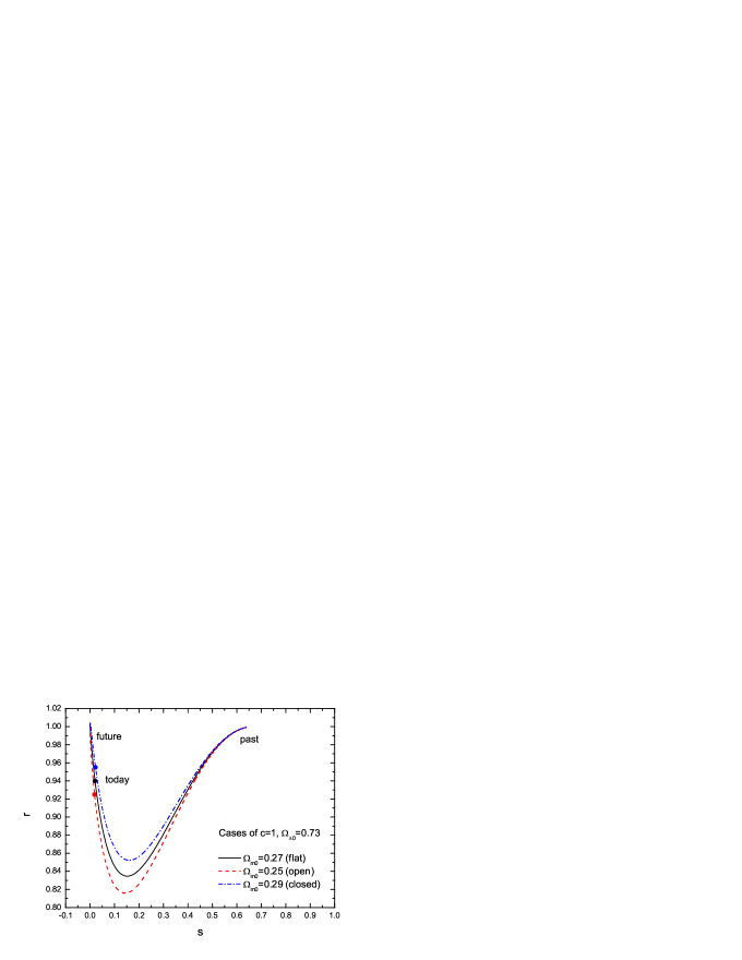
$\begin{array}[]{c@{\hspace{0.2in}}c}\lx@intercol\mbox{}\hfil\lx@intercol&\lx@intercol\mbox{}\hfil\lx@intercol\\ \includegraphics[scale={0.8}]{fig1b.eps}\hfil\hskip 14.45377pt&\includegraphics[scale={0.8}]{fig1c.eps}\\ \end{array}$

Figure 1: An illustrative example for the statefinder diagnosis of the holographic dark energy model. We plot the statefinder diagrams in the $s-r$ plane for the cases $c=1$, $c=0.8$ and $c=1.2$, respectively. Selected curves of $r(s)$ are plotted by fixing $\Omega_{\Lambda 0}=0.73$ and varying $\Omega_{\rm m0}$ as 0.27, 0.25 and 0.29 corresponding to the flat, open and closed universes, respectively. Dots locate the today’s values of the statefinder parameters $(s_{0},r_{0})$.

$\begin{array}[]{c@{\hspace{0.2in}}c}\lx@intercol\mbox{}\hfil\lx@intercol&\lx@intercol\mbox{}\hfil\lx@intercol\\ \includegraphics[scale={0.8}]{fig2a.eps}\hfil\hskip 14.45377pt&\includegraphics[scale={0.8}]{fig2b.eps}\\ \end{array}$

Figure 2: The statefinder diagrams $r(s)$ and $r(q)$ for the spatially non-flat holographic dark energy model. The diagrams are plotted in the light of the best-fit result of the SN+CMB data analysis, $c=0.84$, $\Omega_{\rm m0}=0.29$, and $\Omega_{k0}=0.02$. The coordinates of today locate at: $(s_{0},r_{0})=(-0.102,1.357)$ and $(q_{0},r_{0})=(-0.590,1.357)$. For comparison, the statefinder diagrams for $\Lambda$CDM model (in both spatially flat and non-flat cases) are also plotted in the $s-r$ and $q-r$ planes. The parameters for non-flat $\Lambda$CDM are also $\Omega_{\rm m0}=0.29$ and $\Omega_{k0}=0.02$, and the parameter for flat $\Lambda$CDM is $\Omega_{\rm m0}=0.27$.

On the other hand, associated with the current constraints for the model from the observational data one can predict the statefinder evolution trajectories $r(s)$ and $r(q)$ for the holographic dark energy model. Due to the fact that the cases of flat universe have been analyzed in detail in Ref.[44], we shall discuss the case of non-flat universe here. As has been mentioned above, the analysis of the current observational data involving the information of SNIa and CMB gives the 1-$\sigma$ fit values of the parameters: $c=0.84^{+0.16}_{-0.03}$, $\Omega_{\rm m0}=0.29^{+0.06}_{-0.08}$, and $\Omega_{k0}=0.02\pm 0.10$. We should have analyzed the cosmological evolution of the model with errors of confidence level by means of the statefinder parameters, however, it can be seen clearly that the errors for $\Omega_{k0}$ are very large ($\Omega_{k0}=0.02\pm 0.10$), so that plotting evolution diagrams for statefinder parameters with confidence level errors might not result in any useful information. Thus, we only discuss the best-fit case, which is sufficient for our analysis. Using the best-fit values, we plot in figure 2 the statefinder diagrams $r(s)$ and $r(q)$ for the spatially non-flat holographic dark energy model. The coordinates of today in the holographic dark energy model locate at: $(s_{0},r_{0})=(-0.102,1.357)$ and $(q_{0},r_{0})=(-0.590,1.357)$. For comparison, we also plot the statefinder diagrams of the $\Lambda$CDM model in both spatially flat and non-flat cases in this figure. The parameters for non-flat $\Lambda$CDM are also $\Omega_{\rm m0}=0.29$ and $\Omega_{k0}=0.02$, and the parameter for flat $\Lambda$CDM is $\Omega_{\rm m0}=0.27$. We see clearly that in the $s-r$ plane the flat $\Lambda$CDM is shown as a fixed point $(0,1)$ and the non-flat $\Lambda$CDM is exhibited as a vertical line segment (very short in this plot) with present coordinate $(0,1.02)$; in the $q-r$ plane the flat $\Lambda$CDM behaves as a horizontal line segment with present coordinate $(-0.595,1.00)$ and the non-flat $\Lambda$CDM behaves as an arc with present coordinate $(-0.585,1.02)$. Note that the true values of $(s_{0},r_{0})$ of the universe should be determined in a model-independent way, we can only pin our hope on the future experiments to achieve this. We strongly expect that the future high-precision experiments (e.g. SNAP) may provide sufficiently large amount of precise data to release the information of statefinders $\{H,q,r,s\}$ in a model-independent manner so as to supply a way of discriminating different cosmological models with or without dark energy.

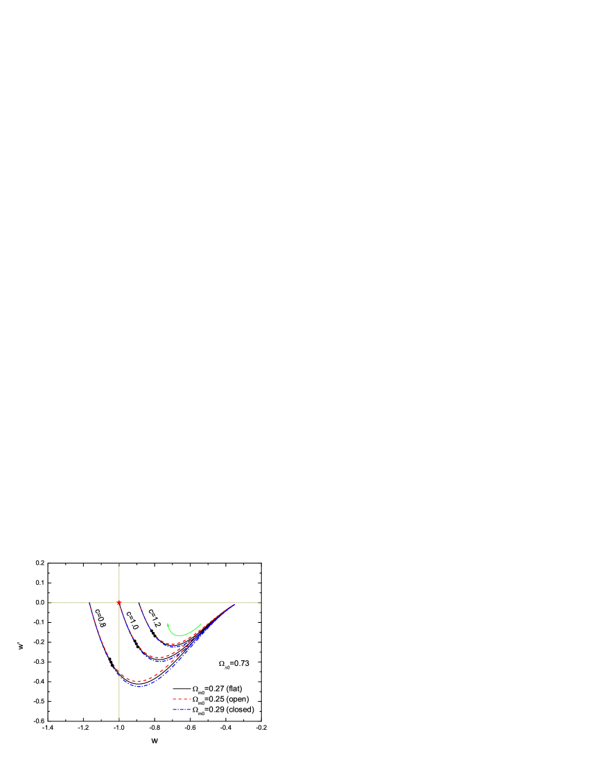
Figure 3: The dynamical evolution behavior of the holographic dark energy in the $w-w^{\prime}$ plane. This diagram shows an illustrative example in which we plot the evolution trajectories of the holographic dark energy model in $w-w^{\prime}$ plane by fixing $\Omega_{\Lambda 0}=0.73$ and varying $\Omega_{\rm m0}$ as 0.27, 0.25 and 0.29 corresponding to the flat, open and closed universes, respectively. Selected curves correspond to $c=1.2$, 1.0 and 0.8 for including various representative cases. The arrow in the diagram denotes the evolution direction. Dots denote the present values of $(w,w^{\prime})$. For comparison, the case for the cosmological constant $\lambda$ is also marked in the $w-w^{\prime}$ plane as a red star.

$\begin{array}[]{c@{\hspace{0.2in}}c}\lx@intercol\mbox{}\hfil\lx@intercol&\lx@intercol\mbox{}\hfil\lx@intercol\\ \includegraphics[scale={0.8}]{fig4a.eps}\hfil\hskip 14.45377pt&\includegraphics[scale={0.8}]{fig4b.eps}\\ \end{array}$

Figure 4: The $s-r$ diagram and the $w-w^{\prime}$ diagram in three cases of evolution of the holographic dark energy in flat and closed universes corresponding to three best-fit results, SN+CMB+BAO and X-ray gas in flat universe, and SN+CMB in non-flat universe. Dots denote the present coordinates.

Also, it is of interest to discuss the dynamical property of the holographic dark energy in the $w-w^{\prime}$ phase plane. Recently, Caldwell and Linder [49] proposed to explore the evolving behavior of quintessence dark energy models and test the limits of quintessence in the $w-w^{\prime}$ plane, where $w^{\prime}$ represents the derivative of $w$ with respect to $\ln a$, and showed that the area occupied by quintessence models in the phase plane can be divided into thawing and freezing regions. Then, it became somewhat popular for analyzing dark energy models in the $w-w^{\prime}$ plane. The method was used to analyze the dynamical property of other dark energy models including more general quintessence models [50], phantom models [51] and quintom models [52], etc.. The $w-w^{\prime}$ analysis undoubtedly provides us with an alternative way of classifying dark energy models using the quantities describing the property of dark energy. But, it is obviously that the $(w,w^{\prime})$ pair is related to statefinder pair $(s,r)$ in a definite way, see Eqs. (23) and (24). The merit of the statefinder diagnosis method roots that the statefinder parameters are constructed from the scale factor $a$ and its derivatives, and they are expected to be extracted in a model-independent way from observational data, although it seems hard to achieve this at present. Now let us investigate the holographic dark energy in the $w-w^{\prime}$ phase plane. Figure 3 shows an illustrative example in which we plot the evolution trajectories of the holographic dark energy model in $w-w^{\prime}$ plane by fixing $\Omega_{\Lambda 0}=0.73$ and varying $\Omega_{\rm m0}$ as 0.27, 0.25 and 0.29 corresponding to the flat, open and closed universes, respectively. Selected curves correspond to $c=1.2$, 1.0 and 0.8 for including various representative cases. The arrow in the diagram denote the evolution direction. We see clearly that the parameter $c$ plays a crucial role in the model: $c\geqslant 1$ makes the holographic dark energy behave as quintessence-type dark energy with $w\geqslant-1$, and $c<1$ makes the holographic dark energy behave as quintom-type dark energy with $w$ crossing $-1$ during the evolution history. As is shown in this diagram that the value of $w$ decreases monotonically while the value of $w^{\prime}$ first decreases from zero to a minimum then increases to zero again. We also notice that the effect of the spatial curvature contribution can be identified explicitly in this diagram. Furthermore, we compare predictions made by different fits of observational data in the $s-r$ plane and the $w-w^{\prime}$ plane. Figure 4 shows the $s-r$ diagram and the $w-w^{\prime}$ diagram in three cases of evolution of the holographic dark energy in flat and closed universes corresponding to three best-fit results, SN+CMB+BAO and X-ray gas in flat universe, and SN+CMB in non-flat universe, as mentioned above. So we see that the $w-w^{\prime}$ dynamical diagnosis can provide us with a useful complement to the statefinder $s-r$ geometrical diagnosis.

In summary, we have in this paper studied the holographic dark energy model in a non-flat universe from the statefinder viewpoint. Since the accelerated expansion of the universe was found by astronomical observations, many cosmological models involving dark energy component or modifying gravity have been proposed to interpret this cosmic acceleration. This leads to a problem of how to discriminate between these various contenders. The statefinder diagnosis provides a useful tool to break the possible degeneracy of different cosmological models by constructing the parameters $\{r,s\}$ using the higher derivative of the scale factor. So the method of plotting the evolution trajectories of dark energy models in the statefinder plane can be used to as a diagnostic tool to discriminate between different models. Furthermore, the values of $\{r,s\}$ of today, if can be extracted from precise observational data in a model-independent way, can be viewed as a discriminator in testing the various cosmological models. On the other hand, though we are lacking an underlying theory of the dark energy, this theory is presumed to possess some features of a quantum gravity theory, which can be explored speculatively by taking the holographic principle of quantum gravity theory into account. So the holographic dark energy model provides us with an attempt to explore the essence of dark energy within a framework of fundamental theory. We perform a statefinder diagnosis for the holographic dark energy model in a non-flat universe in this paper. The statefinder diagrams show that the contributions of the spatial curvature in the model can be diagnosed out explicitly in this method. We hope that the future high-precision observations such as the SNAP-type experiment may be capable of providing large amount of accurate data to determine the statefinder parameters precisely and consequently single out right cosmological models.

References

-
[1]
A. G. Riess et al. [Supernova Search Team Collaboration],
Astron. J. 116, 1009 (1998)
[astro-ph/9805201];
S. Perlmutter et al. [Supernova Cosmology Project Collaboration], Astrophys. J. 517, 565 (1999) [astro-ph/9812133];
P. Astier et al., Astron. Astrophys. 447, 31 (2006) [astro-ph/0510447]. -
[2]
M. Tegmark et al. [SDSS Collaboration],
Phys. Rev. D 69, 103501 (2004)
[astro-ph/0310723];
K. Abazajian et al. [SDSS Collaboration], Astron. J. 128, 502 (2004) [astro-ph/0403325];
K. Abazajian et al. [SDSS Collaboration], Astron. J. 129, 1755 (2005) [astro-ph/0410239]. -
[3]
D. N. Spergel et al. [WMAP Collaboration],
Astrophys. J. Suppl. 148, 175 (2003)
[astro-ph/0302209];
D. N. Spergel et al., astro-ph/0603449. - [4] A. Einstein, Sitzungsber. Preuss. Akad. Wiss. Berlin (Math. Phys.) 1917, 142 (1917).
-
[5]
S. Weinberg,
Rev. Mod. Phys. 61 1 (1989);
V. Sahni and A. A. Starobinsky, Int. J. Mod. Phys. D 9, 373 (2000) [astro-ph/9904398];
S. M. Carroll, Living Rev. Rel. 4 1 (2001) [astro-ph/0004075];
P. J. E. Peebles and B. Ratra, Rev. Mod. Phys. 75 559 (2003) [astro-ph/0207347];
T. Padmanabhan, Phys. Rept. 380 235 (2003) [hep-th/0212290];
E. J. Copeland, M. Sami and S. Tsujikawa, Int. J. Mod. Phys. D 15 (2006) 1753 [hep-th/0603057]. - [6] P. J. Steinhardt, in Critical Problems in Physics, edited by V. L. Fitch and D. R. Marlow (Princeton University Press, Princeton, NJ, 1997).
-
[7]
P. J. E. Peebles and B. Ratra,
Astrophys. J. 325 L17 (1988);
B. Ratra and P. J. E. Peebles, Phys. Rev. D 37 3406 (1988);
C. Wetterich, Nucl. Phys. B 302 668 (1988);
J. A. Frieman, C. T. Hill, A. Stebbins and I. Waga, Phys. Rev. Lett. 75, 2077 (1995) [astro-ph/9505060];
M. S. Turner and M. J. White, Phys. Rev. D 56, 4439 (1997) [astro-ph/9701138];
R. R. Caldwell, R. Dave and P. J. Steinhardt, Phys. Rev. Lett. 80, 1582 (1998) [astro-ph/9708069];
A. R. Liddle and R. J. Scherrer, Phys. Rev. D 59, 023509 (1999) [astro-ph/9809272];
I. Zlatev, L. M. Wang and P. J. Steinhardt, Phys. Rev. Lett. 82, 896 (1999) [astro-ph/9807002];
P. J. Steinhardt, L. M. Wang and I. Zlatev, Phys. Rev. D 59, 123504 (1999) [astro-ph/9812313]. -
[8]
C. Armendariz-Picon, V. F. Mukhanov and P. J. Steinhardt,
Phys. Rev. Lett. 85, 4438 (2000)
[astro-ph/0004134];
C. Armendariz-Picon, V. F. Mukhanov and P. J. Steinhardt, Phys. Rev. D 63, 103510 (2001) [astro-ph/0006373]. -
[9]
A. Sen,
JHEP 0207, 065 (2002)
[hep-th/0203265];
T. Padmanabhan, Phys. Rev. D 66, 021301 (2002) [hep-th/0204150]. -
[10]
R. R. Caldwell,
Phys. Lett. B 545, 23 (2002)
[astro-ph/9908168];
R. R. Caldwell, M. Kamionkowski and N. N. Weinberg, Phys. Rev. Lett. 91, 071301 (2003) [astro-ph/0302506]
S. Nojiri and S. D. Odintsov, Phys. Lett., B 562, 147, (2003);
S. Nojiri and S. D. Odintsov, Phys. Lett., B 565, 1, (2003). - [11] N. Arkani-Hamed, H. C. Cheng, M. A. Luty and S. Mukohyama, JHEP 0405, 074 (2004) [hep-th/0312099].
- [12] F. Piazza and S. Tsujikawa, JCAP 0407, 004 (2004) [hep-th/0405054].
-
[13]
B. Feng, X. L. Wang and X. M. Zhang,
Phys. Lett. B 607, 35 (2005)
[astro-ph/0404224];
Z. K. Guo, Y. S. Piao, X. M. Zhang and Y. Z. Zhang, Phys. Lett. B 608, 177 (2005) [astro-ph/0410654];
X. Zhang, Commun. Theor. Phys. 44, 762 (2005);
H. Wei, R. G. Cai and D. F. Zeng, Class. Quant. Grav. 22, 3189 (2005) [hep-th/0501160];
A. Anisimov, E. Babichev and A. Vikman, JCAP 0506, 006 (2005) [astro-ph/0504560];
M. R. Setare, Phys. Lett. B 641, 130, (2006). -
[14]
L. Amendola,
Phys. Rev. D 62, 043511 (2000)
[astro-ph/9908023];
D. Comelli, M. Pietroni and A. Riotto, Phys. Lett. B 571, 115 (2003) [hep-ph/0302080];
X. Zhang, Mod. Phys. Lett. A 20, 2575 (2005) [astro-ph/0503072];
M. Szydlowski, Phys. Lett. B 632, 1 (2006) [astro-ph/0502034];
M. Szydlowski, A. Kurek, and A. Krawiec Phys. Lett. B 642, 171 (2006) [astro-ph/0604327];
Z. G. Huang, H. Q. Lu and W. Fang, Class. Quant. Grav. 23, 6215 (2006) [hep-th/0604160]. -
[15]
C. Deffayet, G. R. Dvali and G. Gabadadze,
Phys. Rev. D 65, 044023 (2002)
[astro-ph/0105068];
V. Sahni and Y. Shtanov, JCAP 0311, 014 (2003) [astro-ph/0202346]. - [16] A. Y. Kamenshchik, U. Moschella and V. Pasquier, Phys. Lett. B 511, 265 (2001) [gr-qc/0103004].
- [17] S. Kachru, R. Kallosh, A. Linde and S. P. Trivedi, Phys. Rev. D 68, 046005 (2003) [hep-th/0301240].
- [18] L. Susskind, hep-th/0302219.
- [19] E. Witten, hep-ph/0002297.
- [20] A. G. Cohen, D. B. Kaplan and A. E. Nelson, Phys. Rev. Lett. 82, 4971 (1999) [hep-th/9803132].
-
[21]
P. Horava and D. Minic,
Phys. Rev. Lett. 85, 1610 (2000)
[hep-th/0001145];
S. D. Thomas, Phys. Rev. Lett. 89, 081301 (2002). - [22] S. D. H. Hsu, Phys. Lett. B 594, 13 (2004) [hep-th/0403052].
- [23] M. Li, Phys. Lett. B 603, 1 (2004) [hep-th/0403127].
-
[24]
G. ’t Hooft,
gr-qc/9310026;
L. Susskind, J. Math. Phys. 36, 6377 (1995) [hep-th/9409089]. -
[25]
J. D. Bekenstein, Phys. Rev. D 7 (1973) 2333;
J. D. Bekenstein, Phys. Rev. D 9 (1974) 3292; J. D. Bekenstein, Phys. Rev. D 23 (1981) 287;
J. D. Bekenstein, Phys. Rev. D 49 (1994) 1912;
S. W. Hawking, Commun. Math. Phys. 43 (1975) 199;
S. W. Hawking, Phys. Rev. D 13 (1976) 191. - [26] X. Zhang and F. Q. Wu, Phys. Rev. D 72, 043524 (2005) [astro-ph/0506310].
- [27] Z. Chang, F. Q. Wu and X. Zhang, Phys. Lett. B 633, 14 (2006) [astro-ph/0509531].
-
[28]
Q. G. Huang and Y. G. Gong,
JCAP 0408, 006 (2004)
[astro-ph/0403590];
K. Enqvist, S. Hannestad and M. S. Sloth, JCAP 0502 004 (2005) [astro-ph/0409275];
J. Shen, B. Wang, E. Abdalla and R. K. Su, Phys. Lett. B 609 200 (2005) [hep-th/0412227];
H. C. Kao, W. L. Lee and F. L. Lin, Phys. Rev. D 71 123518 (2005) [astro-ph/0501487]. - [29] Q. G. Huang and M. Li, JCAP 0408, 013 (2004) [astro-ph/0404229].
-
[30]
K. Enqvist and M. S. Sloth,
Phys. Rev. Lett. 93, 221302 (2004)
[hep-th/0406019];
K. Ke and M. Li, Phys. Lett. B 606, 173 (2005) [hep-th/0407056];
Q. G. Huang and M. Li, JCAP 0503, 001 (2005) [hep-th/0410095];
D. Pavon and W. Zimdahl, Phys. Lett. B 628, 206 (2005) [gr-qc/0505020];
B. Wang, Y. Gong and E. Abdalla, Phys. Lett. B 624, 141 (2005) [hep-th/0506069];
H. Kim, H. W. Lee and Y. S. Myung, Phys. Lett. B 632, 605 (2006) [gr-qc/0509040];
S. Nojiri and S. D. Odintsov, Gen. Rel. Grav. 38, 1285 (2006) [hep-th/0506212];
E. Elizalde, S. Nojiri, S. D. Odintsov and P. Wang, Phys. Rev. D 71, 103504 (2005) [hep-th/0502082];
B. Hu and Y. Ling, Phys. Rev. D 73, 123510 (2006) [hep-th/0601093];
H. Li, Z. K. Guo and Y. Z. Zhang, Int. J. Mod. Phys. D 15, 869 (2006) [astro-ph/0602521];
X. Zhang, astro-ph/0604484;
M. R. Setare and S. Shafei, JCAP 0609, 011 (2006) [gr-qc/0606103];
M. R. Setare, Phys. Lett. B 642, 1 (2006) [hep-th/0609069];
M. R. Setare, Phys. Lett. B 642, 421 (2006) [hep-th/0609104];
M. R. Setare, hep-th/0610190;
X. Zhang, Phys. Rev. D 74, 103505 (2006) [astro-ph/0609699]. - [31] V. Sahni, T. D. Saini, A. A. Starobinsky and U. Alam, JETP Lett. 77, 201 (2003) [astro-ph/0201498].
- [32] Y. G. Gong, B. Wang and Y. Z. Zhang, Phys. Rev. D 72, 043510 (2005) [hep-th/0412218].
- [33] A. G. Riess et al. [Supernova Search Team Collaboration], Astrophys. J. 607, 665 (2004) [astro-ph/0402512].
- [34] D. J. Eisenstein et al. [SDSS Collaboration], Astrophys. J. 633, 560 (2005) [astro-ph/0501171].
- [35] S. W. Allen, R. W. Schmidt, H. Ebeling, A. C. Fabian and L. van Speybroeck, Mon. Not. Roy. Astron. Soc. 353, 457 (2004) [arXiv:astro-ph/0405340].
- [36] A. K. D. Evans, I. K. Wehus, O. Gron and O. Elgaroy, Astron. Astrophys. 430, 399 (2005) [astro-ph/0406407].
- [37] U. Alam, V. Sahni, T. D. Saini and A. A. Starobinsky, Mon. Not. Roy. Astron. Soc. 344, 1057 (2003) [astro-ph/0303009].
- [38] V. Gorini, A. Kamenshchik and U. Moschella, Phys. Rev. D 67, 063509 (2003) [astro-ph/0209395].
- [39] W. Zimdahl and D. Pavon, Gen. Rel. Grav. 36, 1483 (2004) [gr-qc/0311067].
- [40] V. Sahni, Lect. Notes Phys. 653, 141 (2004) [astro-ph/0403324].
- [41] X. Zhang, F. Q. Wu and J. Zhang, JCAP 0601, 003 (2006) [astro-ph/0411221].
- [42] X. Zhang, Commun. Theor. Phys. 44, 573 (2005).
- [43] X. Zhang, Phys. Lett. B 611, 1 (2005) [astro-ph/0503075].
- [44] X. Zhang, Int. J. Mod. Phys. D 14, 1597 (2005) [astro-ph/0504586].
- [45] M. P. Dabrowski, Phys. Lett. B 625, 184 (2005) [gr-qc/0505069].
- [46] P. X. Wu and H. W. Yu, Int. J. Mod. Phys. D 14, 1873 (2005) [gr-qc/0509036].
- [47] M. G. Hu and X. H. Meng, Phys. Lett. B 635, 186 (2006) [astro-ph/0511615].
- [48] V. Sahni and A. Starobinsky, astro-ph/0610026.
- [49] R. R. Caldwell and E. V. Linder, Phys. Rev. Lett. 95, 141301 (2005) [astro-ph/0505494].
- [50] R. J. Scherrer, Phys. Rev. D 73, 043502 (2006) [astro-ph/0509890].
- [51] T. Chiba, Phys. Rev. D 73, 063501 (2006) [astro-ph/0510598].
- [52] Z. K. Guo, Y. S. Piao, X. Zhang and Y. Z. Zhang, astro-ph/0608165.