Gravastars supported by nonlinear electrodynamics

Abstract

Gravastar models have recently been proposed as an alternative to black holes, mainly to avoid the problematic issues associated with event horizons and singularities. In this work, a wide variety of gravastar models within the context of nonlinear electrodynamics are constructed. Using the $F$ representation, specific forms of Lagrangians are considered describing magnetic gravastars, which may be interpreted as self-gravitating magnetic monopoles with charge $g$. Using the dual $P$ formulation of nonlinear electrodynamics, electric gravastar models are constructed by considering specific structural functions, and the characteristics and physical properties of the solutions are further explored. These interior nonlinear electrodynamic geometries are matched to an exterior Schwarzschild spacetime at a junction interface.

1 Introduction

The generally well-accepted notion of a black hole is deeply rooted in the general relativist community, although a considerable number of particle and condensed matter physicists view the respective notion of event horizons with some suspicion and alarm [1, 2, 3]. In addition to this, one still encounters the existence of misconceptions and a certain ambiguity inherent to the Schwarzschild solution in the literature (see Ref. [4] for a review). Despite the fact that the evidence of the existence of black holes in the Universe is very convincing, a certain amount of scepticism regarding the observational data is still encountered [5]. This scepticism has inspired new and fascinating ideas. In particular, models replacing the interior Schwarzschild solution with compact objects, and thus, doing away with the problems of the singularity at the origin and the event horizon, have been proposed to some extent in the literature. However, we do emphasize that the interior structure of realistic black holes has not been satisfactorily determined, and is still open to considerable debate. In this line of thought, an interesting alternative to black holes has recently been proposed, namely, the “gravastar” (gravitational vacuum star) picture developed by Mazur and Mottola [2]. In this model, and in the related picture developed by Laughlin et al [1], the quantum vacuum undergoes a phase transition at or near the location where the event horizon is expected to form. The Mazur-Mottola model is constituted by an onion-like structure with five layers, including two thin-shells, with surface stresses $\sigma_{\pm}$ and ${\cal P}_{\pm}$, where $\sigma$ is the surface energy density and ${\cal P}$ is the surface tangential pressure. The interior of the solution is replaced by a segment of de Sitter space, which is then matched to a finite thickness shell of stiff matter with the equation of state $p=\rho$. The latter is then matched to an external Schwarzschild vacuum with $p=\rho=0$. Related models, analyzed in a different context have also been considered by Dymnikova [6].

Although Mazur and Mottola argued for the thermodynamic stability of their configuration, the full dynamic stability against spherically symmetric perturbations was carried out in Ref. [7], through a simplified construction of the Mazur-Mottola model. The configuration was simplified to a three-layer solution, i.e., a de Sitter interior solution was matched to a Schwarzschild exterior solution at a junction surface, comprising of a thin shell with surface stresses $\sigma$ and ${\cal P}$. It was found that many equations of state exist that imply the dynamical stability of the gravastar configurations. The latter dynamical stability was generalized to an anti-de Sitter or de Sitter interior and a Schwarzschild-(anti)-de Sitter or Reissner–Nordström exterior [8]. In Ref. [9], by disregarding the presence of thin shells, a generalized class of gravastar models was analyzed. It was found, using these models, that gravastars cannot be perfect fluid spheres, and that they necessarily exhibit anisotropic pressures. Specific stable solutions, with respect to axial perturbations, possessing continuous pressures were also further explored [10]. In this context, one may also replace the interior de Sitter spacetime with a solution governed by the dark energy equation of state, $\omega=p/\rho$, where $\omega<-1/3$ [11]. Note that the particular case of $\omega=-1$ reduces to the de Sitter solution, and for $\omega<-1$, one ends up with phantom energy, an exotic cosmic fluid which violates the null energy condition. Now, the notion of dark energy is that of a spatially homogeneous cosmic fluid, however, inhomogeneities may arise through gravitational instabilities. Thus, these inhomogeneous solutions, denoted as dark energy stars [3, 11], may possibly originate from density fluctuations in the cosmological background. Note that now the pressure in the equation of state $p=\omega\rho$ is a radial pressure, and the transverse pressure may be determined from the field equations, as emphasized in Refs. [12], in a rather different context.

In Ref. [13], motivated by low energy string theory, an alternative model was constructed by replacing the de Sitter regime with an interior solution governed by a Chaplygin gas equation of state, interpreted as a Born-Infeld phantom gravastar. In this context, the extension of the latter Born-Infeld gravastar variation to rather more general nonlinear electrodynamic models shall prove extremely interesting, and this is, in fact the analysis of the present paper. It is interesting to note that nonlinear electrodynamics has recently been revived, mainly due to the fact that these models appear as effective theories at different levels of string/M-theory, in particular, in D$p-$branes and supersymmetric extensions, and non-Abelian generalizations (we refer the reader to Ref. [14] for a review), and have enjoyed a wide variety of applicability, namely, in cosmology [15]. Traversable wormholes have also been explored in nonlinear electrodynamics [16, 17]. It was found that regular pure magnetic evolving wormholes exist [16]. However, static spherically symmetric and stationary axisymmetric traversable wormholes have been ruled out, mainly due to the presence of event horizons, the non-violation of the null energy condition at the throat, and due to the imposition of the principle of finiteness, which states that a satisfactory theory should avoid physical quantities becoming infinite [17]. In fact, the Born-Infeld model was inspired mainly on the principle of finiteness, in order to remedy the fact that the standard picture of a point particle possesses an infinite self-energy [18]. Later, Plebański presented other examples of nonlinear electrodynamic Lagrangians [19], and showed that the Born-Infeld theory satisfies physically acceptable requirements.

It was in nonlinear electrodynamics that the first exact regular black hole solutions to the Einstein field equation were found [20, 21, 22]. In this context, magnetic black holes and monopoles [23], regular electrically charged black holes of a hybrid type containing a magnetically charged core [24], and electrically charged structures with a regular de Sitter center [25], have been found. In this work, we are interested in the construction of a wide variety of gravastar models coupled to nonlinear electrodynamics. Using the $F$ representation, we consider specific forms of Lagrangians describing magnetic gravastars, which may be interpreted as self-gravitating magnetic monopoles with a charge $g$. Using the $P$ formulation of nonlinear electrodynamics, it is easier to find electric solutions, and considering specific structural functions we further explore the characteristics and physical properties of the solutions. We match these interior nonlinear electrodynamic geometries to an exterior Schwarzschild spacetime, thus avoiding the problematic issues related to the singularities and event horizons.

This paper is organized in the following manner: In section 2, we outline the field equations, and analyze some characteristics of the solutions. In section 3, we consider the $F$ representation of nonlinear electrodynamics, and explore specific magnetic solutions in some detail. In section 4, we outline the dual $P$ formalism and extensively analyze electric gravastar solutions. In section 5, we conclude.

2 Field equations

We consider the action of $(3+1)-$dimensional general relativity coupled to nonlinear electrodynamics given in the following form

$$S=\int\sqrt{-g}\left[\frac{R}{16\pi}+L(F)\right]\,d^{4}x\,,$$ (1)

where $R$ is the Ricci scalar, and $L(F)$ is a gauge-invariant electromagnetic Lagrangian. The latter depends on a single invariant $F$ given by $F=F^{\mu\nu}F_{\mu\nu}/4$ [19], where the antisymmetric tensor $F_{\mu\nu}=A_{\nu,\mu}-A_{\mu,\nu}$ is the electromagnetic field. In Einstein-Maxwell theory, the Lagrangian takes the form $L(F)=-F/4\pi$. However, we consider more general choices for the electromagnetic Lagrangians. Note that the Lagrangian may also be constructed using a second invariant $G\sim F_{\mu\nu}{}^{*}F^{\mu\nu}$, where the asterisk ^∗ denotes the Hodge dual with respect to $g_{\mu\nu}$. However, we only consider $F$, as this provides solutions that are interesting enough.

Varying the action with respect to the gravitational field provides the Einstein field equations $G_{\mu\nu}=8\pi T_{\mu\nu}$, where $G_{\mu\nu}$ is the Einstein tensor, and the stress-energy tensor, $T_{\mu\nu}$, is given by

$$T_{\mu\nu}=g_{\mu\nu}\,L(F)-F_{\mu\alpha}F_{\nu}{}^{\alpha}\,L_{F}\,.$$ (2)

with $L_{F}=dL/dF$.

The electromagnetic field equations are the following

$$\left(F^{\mu\nu}\,L_{F}\right)_{;\mu}=0\;,\qquad\left({}^{*}F^{\mu\nu}\right)_{;\mu}=0\,.$$ (3)

The first equation may be obtained by varying the action with respect to the electromagnetic potential $A_{\mu}$. The second relationship, in turn, may be obtained from the Bianchi identities.

Consider a static and spherically symmetric spacetime, in curvature coordinates, given by the following line element

$$ds^{2} = -e^{2\alpha(r)}\,dt^{2}+e^{2\beta(r)}\,dr^{2}+r^{2}(d\theta^{2}+\sin^{2}{\theta}\,d\phi^{2})\,,$$ (4)

where $\alpha$ and $\beta$ are functions of $r$.

Taking into account the symmetries of the geometry, the non-zero compatible terms for the electromagnetic tensor are

$$F_{\mu\nu}=2E(x^{\alpha})\,\delta^{[t}_{\mu}\,\delta^{r]}_{\nu}+2B(x^{\alpha})\,\delta^{[\theta}_{\mu}\,\delta^{\phi]}_{\nu}\,,$$ (5)

so that the only non-zero terms are $F_{tr}=E(x^{\mu})$ and $F_{\theta\phi}=B(x^{\mu})$.

The Einstein tensor components, in an orthonormal reference frame, (with $c=G=1$) are given by

$$G_{\hat{t}\hat{t}} = \;\frac{e^{-2\beta}}{r^{2}}\,\left(2\beta^{\prime}r+e^{2\beta}-1\right)\,,$$ (6)

$$G_{\hat{r}\hat{r}} = \frac{e^{-2\beta}}{r^{2}}\,\left(2\alpha^{\prime}r-e^{2\beta}+1\right)\,,$$ (7)

$$G_{\hat{\phi}\hat{\phi}} = G_{\hat{\theta}\hat{\theta}}=\frac{e^{-2\beta}}{r}\,\left[-\beta^{\prime}+\alpha^{\prime}+r\alpha^{\prime\prime}+r(\alpha^{\prime})^{2}-r\alpha^{\prime}\beta^{\prime}\right]\,,$$ (8)

where the prime denotes a derivative with respect to the radial coordinate, $r$. Now, it is a simple matter, using equation (2) in an orthonormal reference frame, to verify that $T_{\hat{t}\hat{t}}=-T_{\hat{r}\hat{r}}$. Thus, using the Einstein field equation, and taking into account equations (6) and (7), we have $\alpha^{\prime}+\beta^{\prime}=0$, which provides the solution $\alpha=-\beta+C$. The constant $C$ may be absorbed by defining a new time coordinate, so that without a loss of generality, we may consider $C=0$.

For notational and computational convenience, we consider the metric fields in the following form

$$e^{2\alpha(r)}=e^{-2\beta(r)}=\left[1-\frac{2m(r)}{r}\right]\,,$$ (9)

so that the Einstein tensor components reduce to

$$G_{\hat{t}\hat{t}}=-G_{\hat{r}\hat{r}}=\frac{2m^{\prime}}{r^{2}}\,,\qquad G_{\hat{\phi}\hat{\phi}}=G_{\hat{\theta}\hat{\theta}}=-\frac{m^{\prime\prime}}{r}\,.$$ (10)

The function $m(r)$ may be considered the quasi-local mass, and is denoted as the mass function. The stress-energy tensor, in the orthonormal reference frame, assumes the diagonal form $T_{\hat{\mu}\hat{\nu}}={\rm diag}(\rho,p_{r},p_{t},p_{t})$, in which $\rho(r)$ is the energy density, $p_{r}(r)$ is the radial pressure, and $p_{t}(r)$ is the lateral pressure measured in the orthogonal direction to the radial direction. Thus, the Einstein field equations finally take the form

$$\rho(r) = -p_{r}(r)=-L-E^{2}L_{F}=\frac{1}{4\pi}\;\frac{m^{\prime}}{r^{2}}\,,$$ (11)

$$p_{t}(r) = L-\frac{1}{r^{4}\sin^{2}\theta}\,B^{2}\,L_{F}=-\frac{1}{8\pi}\;\frac{m^{\prime\prime}}{r}\,.$$ (12)

We will consider $|E^{2}\,L_{F}|<\infty$ and $|B^{2}\,L_{F}/(r^{4}\sin^{2}\theta)|<\infty$, as $r\rightarrow 0$, to ensure the regularity of the stress-energy tensor components.

One may now define the factor $\alpha^{\prime}(r)$ as the gravity profile, as it is related to the radial component of proper acceleration that an observer must maintain in order to remain at rest at constant $r$, $\theta$, $\phi$. Note that the radial component of proper acceleration is given by $a^{r}=(1-2m(r)/r)\,\alpha^{\prime}(r)$ (see Ref. [26] for details). Thus, the convention used is that $\alpha^{\prime}(r)$ is positive for an inwardly gravitational attraction, and negative for an outward gravitational repulsion [26]. For gravastars an essential condition is that they have a repulsive nature, i.e., $\alpha^{\prime}<0$, which for the present case amounts to imposing the following condition

$$\alpha^{\prime}(r)=\frac{m(r)-m^{\prime}(r)r}{r[r-2m(r)]}<0\,.$$ (13)

We emphasize that what is required from a spherically symmetric solution of the Einstein equations to be a gravastar model, is the presence of a repulsive nature of the interior solution, which is characterized by the notion of the “gravity profile”. The interior solution is then matched to an exterior Schwarzschild solution which is outlined further ahead.

We also explore the energy conditions, in particular, the weak energy condition (WEC), which is defined as $T_{\hat{\mu}\hat{\nu}}U^{\hat{\mu}}U^{\hat{\nu}}\geq 0$ where $U^{\hat{\mu}}$ is a timelike vector. The fact that the stress energy tensor is diagonal will be helpful, so that the following three conditions are imposed

$$\rho\geq 0\,,\qquad\rho+p_{r}\geq 0\,,\qquad\rho+p_{t}\geq 0\,.$$ (14)

From the first inequality, we verify that $m^{\prime}\geq 0$ is imposed. Note that $\rho+p_{r}=0$, so that the second inequality is readily satisfied. Relatively to the third inequality, consider the factor

$$\rho+p_{t}=-\left(E^{2}+\frac{1}{r^{4}\sin^{2}\theta}\,B^{2}\right)\;L_{F}=\frac{N(r)}{8\pi r^{2}}\,,$$ (15)

where for simplicity, $N(r)$ is defined as

$$N(r)=2m^{\prime}-rm^{\prime\prime}\,.$$ (16)

Thus, in summary, to ensure the WEC, we simply need to impose that

$$m^{\prime}\geq 0\qquad{\rm and}\qquad N(r)\geq 0$$ (17)

throughout the spacetime.

In the present case, the term $\rho+p_{t}$ is equivalent to the anisotropy factor which is defined as $\Delta=p_{t}-p_{r}$. The latter is a measure of the pressure anisotropy of the fluid comprising the gravastar. $\Delta=0$ corresponds to the particular case of an isotropic pressure gravastar, which in our case reduces to the trivial case of $E=B=0$, as may be verified from equation (15). Note that $\Delta/r$ represents a force due to the anisotropic nature of the stellar model, which is repulsive, i.e., being outward directed if $p_{t}>p_{r}$, and attractive if $p_{t}<p_{r}$.

We consider a cut-off of the stress-energy tensor at a junction radius $a$, much in the spirit of the original Mazur-Mottola gravastar model [2]. For instance, consider for simplicity that the exterior solution is the Schwarzschild spacetime, given by

$$ds^{2} = -\left(1-\frac{2M}{r}\right)\,dt^{2}+\left(1-\frac{2M}{r}\right)^{-1}dr^{2}+r^{2}(d\theta^{2}+\sin^{2}{\theta}\,d\phi^{2})\,.$$ (18)

$M$ may be interpreted as the gravastar’s total mass. In this case the spacetimes given by the metrics (4) and (18) are matched at $a$, and one has a thin shell surrounding the gravastar. Note that to avoid the presence of an event horizon, we need to impose $a>2M$. Using the Darmois-Israel formalism, the surface stresses are given by

$$\sigma = -\frac{1}{4\pi a}\left(\sqrt{1-\frac{2M}{a}+\dot{a}^{2}}-\sqrt{1-\frac{2m}{a}+\dot{a}^{2}}\,\right),$$ (19)

$${\cal P} = \frac{1}{8\pi a}\left(\frac{1-\frac{M}{a}+\dot{a}^{2}+a\ddot{a}}{\sqrt{1-\frac{2M}{a}+\dot{a}^{2}}}-\frac{1-\frac{m}{a}-m^{\prime}+\dot{a}^{2}+a\ddot{a}}{\sqrt{1-\frac{2m}{a}+\dot{a}^{2}}}\,\right)\,,$$ (20)

where the overdot denotes a derivative with respect to the proper time, $\tau$, and the prime represents, for the present case, a derivative with respect to $a$. $\sigma$ is the surface energy density and ${\cal P}$ the surface pressure (see Refs. [27] for details). The static case is given by taking into account $\dot{a}=\ddot{a}=0$. The total mass of the gravastar, for the static case, with the junction interface $a_{0}$, is given by

$$M=m(a_{0})+m_{s}(a_{0})\left[\sqrt{1-\frac{2m(a_{0})}{a_{0}}}-\frac{m_{s}(a_{0})}{2a_{0}}\right]\,,$$ (21)

where $m_{s}$ is the surface mass of the thin shell, and is defined as $m_{s}=4\pi a^{2}\sigma$.

It is also important to mention that for a self-gravitating object (solution to Einstein’s equations) to be considered as a possible alternative to a black hole, which was one of the original ideas behind the gravastar model, the surface redshift should be able to reach values that are higher than that of ordinary objects. The surface redshift is defined by $Z=\Delta\lambda/\lambda_{e}=\lambda_{0}/\lambda_{e}-1$, where $\Delta\lambda$ is the fractional change between the observed wavelength, $\lambda_{0}$, and the emitted wavelength, $\lambda_{e}$. Thus, according to our notation, the surface value takes the form

$$Z_{a_{0}}=e^{-\alpha(a_{0})}-1\,.$$ (22)

Now, for a static perfect fluid sphere the surface redshift is not larger than $Z=2$ [28]. However, for anisotropic spheres this value may be larger [29]. For the present case of nonlinear electrodynamic gravastars, the bounds on the surface redshift, in principle, place restrictions on the characteristic parameters of the nonlinear electrodynamic theory, which can be analyzed on a case by case, but we will not pursue this here.

3 $F$ representation of nonlinear electrodynamics

A number of nonexistence theorems prohibiting regular electrically charged nonlinear electrodynamic structures have been proposed. These basically state that any $L$ approaching the Maxwell weak field limit, $F\ll 1$, such that $L\sim-F$, prohibit electrically charged static spherically symmetric geometries with a regular center [23]. However, it has been argued that due to the fact that the energy density attains a maximum at the center, the validity of the Maxwell field limit at the center cannot be expected [25]. Another important feature worth mentioning, is that imposing the Maxwell limit at the center and at infinity, inevitably leads to a branching of $L$ as a function of $F$. However, this issue should not bother us, as in this paper we consider matchings of interior nonlinear electrodynamic solutions to an exterior Schwarzschild spacetime, and thus the range considered generally implies a monotonic behavior of $L$ as a function of $F$. As the Maxwellian limit is not imposed at the center, but rather at infinity, the nonlinear electrodynamic constructions outlined in this work do not possess the weak field limit in the specific range of interest, i.e., $0\leq r\leq a$, so that we are at a certain freedom to consider rather general Lagrangians, in particular, those that do not obey the Maxwellian limit for $F\ll 1$.

Now, taking into account the electromagnetic field equations, equations (3), from $\left({}^{*}F^{\mu\nu}\right)_{;\mu}=0$, we obtain $B^{\prime}=0$ and $E_{,\theta}=0$, so that we have $E=E(r)$ and $B=B(\theta)$. From $\left(F^{\mu\nu}\,L_{F}\right)_{;\mu}=0$, we deduce

$$EL_{F}=\frac{q_{e}}{r^{2}}\,,\qquad B=q_{m}\sin\theta\,.$$ (23)

The invariant $F=F^{\mu\nu}F_{\mu\nu}/4$, included for self-completeness, takes the following form

$$F=-\frac{1}{2}\left(E^{2}-\frac{B^{2}}{r^{4}\sin^{2}\theta}\right)=-\frac{1}{2}\left(E^{2}-\frac{q_{m}^{2}}{r^{4}}\right)\,.$$ (24)

Note that from the imposition of the WEC, equation (15) reduces to

$$\rho+p_{t}=-\left(E^{2}+\frac{q_{m}^{2}}{r^{4}}\right)\;L_{F}=\frac{N(r)}{8\pi r^{2}}\,,$$ (25)

from which we verify $L_{F}\leq 0$. Now, from equations (23) and (25), we determine the electric field, $E$, given by

$$E(r)=\frac{1}{16\pi q_{e}}\left[-N(r)\pm\sqrt{N^{2}(r)-\left(\frac{16\pi q_{e}q_{m}}{r^{2}}\right)^{2}}\right]\,.$$ (26)

One verifies that independently of $N(r)$, the electric field diverges at the center. Thus, taking into account the principle of finiteness, which states that a satisfactory theory should avoid physical quantities becoming infinite, the message that one may extract is that for the present geometry, both electric and magnetic fields cannot coexist. One should either consider a pure electric field or a pure magnetic field. We emphasize that the principle of finiteness, which is a basic requisite of nonlinear electrodynamic theory, is related to physically measured entities or physical quantities, independently of the particular basis, as introduced by Born and Infeld and later retaken by Plabanski, such as the electric and magnetic fields. The $F$ is a construct of the formalism, and therefore not the physically measured entity.

3.1 Pure electric field

Considering a pure electric field, $B=0$, and the non-trivial case of the negative sign in equation (26), we have

$$E(r)=-\frac{N(r)}{8\pi q_{e}}\,,\qquad F=-E^{2}/2=-\frac{N^{2}}{2(8\pi q_{e})^{2}}\,.$$ (27)

From $EL_{F}=q_{e}/r^{2}$, the following relationship is deduced

$$L_{F}=-\frac{8\pi q_{e}^{2}}{Nr^{2}}\,,$$ (28)

and the Lagrangian is provided by equation (12), i.e.,

$$L=-\frac{1}{8\pi}\frac{m^{\prime\prime}}{r}\,.$$ (29)

Relatively to the WEC, one may consider a brief analysis by taking into account the nonlinear electrodynamic quantities. From the condition $\rho\geq 0$, we deduce $L\leq 2FL_{F}$, and as noted above, $\rho+p_{r}=0$ is readily verified. From the condition $\rho+p_{t}\geq 0$, we have $FL_{F}\geq 0$, and as $F<0$, then we verify that $L_{F}\leq 0$.

3.2 Pure magnetic field

For a pure magnetic field, $E=0$, we have the following relevant factors

$$B=q_{m}\sin\theta\,,\qquad F=\frac{q_{m}^{2}}{2r^{4}}\,,$$ (30)

and

$$L_{F}=-\frac{Nr^{2}}{8\pi q_{m}^{2}}\,.$$ (31)

Using equation (11), the Lagrangian is given by

$$L=-\frac{1}{4\pi}\frac{m^{\prime}}{r^{2}}\,.$$ (32)

From the above equations, namely, from $F$ and $L$, one verifies that specifying a convenient nonlinear electrodynamic Lagrangian, equation (32) may be integrated to provide the mass function, and thus specifying the geometry of the solution. We explore several cases in some detail in the next section.

Analogously to the previous case, one may analyze the WEC by taking into account the nonlinear electrodynamic quantities. From the inequality $\rho\geq 0$, we have $L\leq 0$. From the condition $\rho+p_{t}\geq 0$, we deduce $-FL_{F}\geq 0$, and as $F\geq 0$, then we verify that $L_{F}\leq 0$.

3.2.1 Magnetic Dymnikova gravastar.

In this section, we analyze the Lagrangian analogue of the structural function, representing a regular electrically charged structure, proposed by Dymnikova [25]. Consider the Lagrangian and its derivative given by

$$L=-\frac{F}{4\pi\left(1+b\sqrt{2q_{m}^{2}F}\right)^{2}}\,,\qquad L_{F}=-\frac{1}{4\pi\left(1+b\sqrt{2q_{m}^{2}F}\right)^{3}}\,,$$ (33)

where $b$ is a characteristic parameter of the nonlinear electrodynamic theory. Note that the stability of this solution has also been analyzed in Ref. [30]. In the weak field limit, $F\ll 1$, the Lagrangian assumes the Einstein-Maxwell form, $L\sim-F/(4\pi)$ and $L_{F}\sim-1/(4\pi)$.

Using $F=q_{m}^{2}/(2r^{4})$, the above relationships take the following form

$$L=-\frac{g^{2}}{8\pi(bg^{2}+r^{2})^{2}}\,,\qquad L_{F}=-\frac{r^{6}}{4\pi(bg^{2}+r^{2})^{3}}\,,$$ (34)

where we consider the definition $g=|q_{m}|$.

Now, using equation (32), one may deduce the mass function, which is given by

$$m(r)=-\frac{g^{2}r}{4\left(bg^{2}+r^{2}\right)}+\frac{g}{4\sqrt{b}}\,\arctan\left(\frac{r}{\sqrt{b}g}\right)\,.$$ (35)

The stress-energy tensor components are given by

$$\rho=-p_{r}=\frac{g^{2}}{8\pi(bg^{2}+r^{2})^{2}}\qquad p_{t}=\frac{g^{2}(r^{2}-bg^{2})}{8\pi(bg^{2}+r^{2})^{3}}\,,$$ (36)

which are regular throughout the spacetime. The WEC is satisfied as can be verified from the following relationships

$$m^{\prime}(r)=\frac{g^{2}r^{2}}{2(bg^{2}+r^{2})^{2}}\,,\qquad N(r)=\frac{2g^{2}r^{4}}{(bg^{2}+r^{2})^{3}}\,,$$ (37)

which are manifestly positive.

The metric fields are given by

$$e^{2\alpha}=e^{-2\beta}=1-\left[-\frac{g^{2}}{2\left(bg^{2}+r^{2}\right)}+\frac{g}{2\sqrt{b}\,r}\,\arctan\left(\frac{r}{\sqrt{b}g}\right)\right]\,.$$ (38)

Defining $y=r/(\sqrt{b}g)$, the above equation provides

$$f(b,y)=1-\frac{1}{2by}\left[\arctan(y)-\frac{y}{1+y^{2}}\right]\,.$$ (39)

Using $\partial f/\partial y=0$, we verify that $f$ possesses a single minimum, $y_{m}\approx 1.825$, independently of the value of $b$. Now, $f(b,y_{m})=0$ has a single positive root at $b\approx 0.1775$. For $b>b_{r}$, we have $f(b,y)>0$. If $b<b_{r}$, then $f(b,y)$ possesses two roots, $y_{1}$ and $y_{2}$, which reflects the existence of event horizons. Note that $f(b,y)>0$ for $y<y_{1}$ and $y>y_{2}$, which are the cases we are interested in. This analysis is represented in figure 1.

Figure 1: Roots of $f(b,y)$, with $b_{1}=0.2775$, $b_{2}=0.1775$ and $b_{3}=0.1075$, respectively. Note the presence of two positive roots, for $b<b_{r}\simeq 0.1775$, reflecting the existence of event horizons. For $b>b_{r}$, we have $f>0$.

Consider the gravity profile written in the following form

$$G(b,y)=g\,b^{3/2}\alpha^{\prime}(b,y)=-\frac{\frac{y(1+3y^{2})}{1+y^{2}}-\arctan(y)}{4y^{2}\left\{1-\frac{1}{2by}\left[\arctan(y)-\frac{y}{1+y^{2}}\right]\right\}}\,,$$ (40)

which is depicted in figure 2. For $b>b_{r}$, we verify that $\alpha^{\prime}<0$, i.e., the gravity profile is negative, reflecting a repulsive character of the geometry, for all values of $y$. For the case of $b<b_{r}$ and for $f>0$, the gravity profile is only negative in the range $y<y_{1}$ and $y>y_{2}$. In the right plot of figure 2, we have considered the specific case of $b=0.0975$.

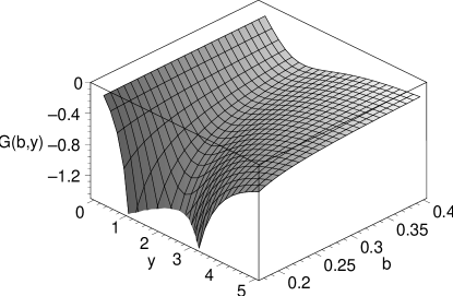
Figure 2: Plots of the gravity profile $G(b,y)=g\,b^{3/2}\alpha^{\prime}(b,y)$. In the left plot, we have considered $b>b_{r}$, and have shown that $\alpha^{\prime}<0$ for all values of $y$. In the right plot, we have the case of $b<b_{r}$ and for $f>0$ the gravity profile is only negative in the range $y<y_{1}$ and $y>y_{2}$. We have considered the specific case of $b=0.0975$. The dashed curves represent the gravity profile and the solid line depicts $f(b,y)$.

Therefore, one may construct a nonlinear electrodynamic magnetic gravastar, by matching the solution outlined above to an exterior Schwarzschild solution. Note, however, that the magnetic permeability, $\mu\sim 1/L_{F}$, diverges at the center, $r=0$, as $L_{F}\rightarrow 0$, thus, exhibiting a magnetically superconductive behavior. For $b>b_{r}$, we verify the absence of event horizons and the gravity profile is negative for all values of $y$, so that the matching occurs simply at $a>2M$. If $b<b_{r}$, then more care needs to be taken due to the presence of two horizons, at $r_{1}=\sqrt{b}\,gy_{1}$ and $r_{2}=\sqrt{b}\,gy_{2}$, respectively. The gravity profile is negative for $r<r_{1}$, so that the matching should be at $r_{1}>a_{0}>2M$, in order to avoid the presence of event horizons. The surface stresses of the thin shell are given by

$$\sigma = -\frac{1}{4\pi a_{0}}\left\{\sqrt{1-\frac{2M}{a_{0}}}-\sqrt{1-\left[-\frac{g^{2}}{2\left(bg^{2}+a_{0}^{2}\right)}+\frac{g}{2\sqrt{b}\,a_{0}}\,\arctan\left(\frac{a_{0}}{\sqrt{b}g}\right)\right]}\,\right\}\,,$$ (41)

$${\cal P} = \frac{1}{8\pi a_{0}}\left\{\frac{1-\frac{M}{a_{0}}}{\sqrt{1-\frac{2M}{a_{0}}}}-\frac{1-\frac{g^{2}(a_{0}^{2}-bg^{2})}{4\left(bg^{2}+a_{0}^{2}\right)}-\frac{g}{4\sqrt{b}\,a_{0}}\,\arctan\left(\frac{a_{0}}{\sqrt{b}g}\right)}{\sqrt{1-\left[-\frac{g^{2}}{2\left(bg^{2}+a_{0}^{2}\right)}+\frac{g}{2\sqrt{b}\,a_{0}}\,\arctan\left(\frac{a_{0}}{\sqrt{b}g}\right)\right]}\,}\right\}\,.$$ (42)

The total mass of the magnetic monopole gravastar is provided by the following relationship

$$M = -\frac{g^{2}a_{0}}{4\left(bg^{2}+a_{0}^{2}\right)}+\frac{g}{4\sqrt{b}}\,\arctan\left(\frac{a_{0}}{\sqrt{b}g}\right)$$ (43)

$$+m_{s}(a_{0})\left[\sqrt{1+\frac{g^{2}}{2\left(bg^{2}+a_{0}^{2}\right)}-\frac{g}{2\sqrt{b}\,a_{0}}\,\arctan\left(\frac{a_{0}}{\sqrt{b}g}\right)}-\frac{m_{s}(a_{0})}{2a_{0}}\right]\,.$$

3.2.2 Magnetic Bardeen gravastar.

Bardeen seems to have been the first author to surprisingly produce a regular black hole model [31]. It is interesting to note that the Bardeen model has been reinterpreted as a magnetic solution to the Einstein field equation coupled to nonlinear electrodynamics [32], i.e., it corresponds to a self-gravitating magnetic monopole. (Gravitational magnetic monopole stellar solutions have also been explored in Majumdar-Papapetrou systems [33]).

Consider the Lagrangian and its derivative, $L_{F}$, written in the following form

$$L=-\frac{3}{4\pi sq_{m}^{2}}\left(\frac{\sqrt{2q_{m}^{2}F}}{1+\sqrt{2q_{m}^{2}F}}\right)^{5/2}\,,\qquad L_{F}=-{\frac{15}{8\pi s}}\,\frac{(2{q_{m}}^{2}F)^{1/4}}{(1+\sqrt{2{q_{m}}^{2}F}\,)^{7/2}}\,.$$ (44)

Note, however, that this Lagrangian does not assume the Maxwell form in the weak field limit, i.e., $L\sim-FF^{1/4}$ for $F\ll 1$. It is perhaps important to emphasize here that to be a nonlinear electrodynamic model, the Maxwellian limit has to be recovered in the weak field limit. The nonexistence theorems, proposed in Ref. [23], of electrically charged regular structures imposed the weak field limit as $r\rightarrow 0$. However, it was argued that as the energy density attains a maximum at the center, the Maxwellian limit cannot be expected at $r=0$ [25]. Note that it is only at $r\rightarrow\infty$ that the weak field limit is recovered $F\rightarrow 0$, for the spacetimes considered in this work. Therefore, in the gravastar models that we construct, it is not necessary to regain the weak field limit in the specified range $0\leq r\leq a$, as the interior nonlinear electrodynamic solution is matched at a junction interface $a$, to an exterior vacuum geometry.

Using $F=q_{m}^{2}/(2r^{4})$, then the above relationships take the form

$$L=-{\frac{3\,g_{B}^{3}}{4\pi s\left({r}^{2}+g_{B}^{2}\right)^{5/2}}}\,,\qquad L_{F}=-{\frac{15\,g_{B}{r}^{6}}{8\pi s\left({r}^{2}+g_{B}^{2}\right)^{7/2}}}\,,$$ (45)

where we consider the definition $g_{B}=|q_{m}|$.

Using equation (32), one may deduce the following mass function, given by

$$m(r)={\frac{g_{B}r^{3}}{s\left({r}^{2}+g_{B}^{2}\right)^{3/2}}}\,.$$ (46)

The stress-energy tensor components are given by

$$\rho=-p_{r}={\frac{3\,g_{B}^{3}}{4\pi s\left({r}^{2}+g_{B}^{2}\right)^{5/2}}}\,,\qquad p_{t}={\frac{3\,g_{B}^{3}\left(3\,{r}^{2}-2\,g_{B}^{2}\right)}{8\pi s\left({r}^{2}+g_{B}^{2}\right)^{7/2}}}\,.$$ (47)

The WEC is satisfied, as may be verified from the following relationships

$$m^{\prime}(r)={\frac{3\,g_{B}^{3}{r}^{2}}{s\left({r}^{2}+g_{B}^{2}\right)^{5/2}}}\,,\qquad N(r)={\frac{15\,g_{B}^{3}{r}^{4}}{s\left({r}^{2}+g_{B}^{2}\right)^{7/2}}}\,.$$ (48)

The metric fields given by $f(r)=1-2m(r)/r$, may be rewritten as

$$f(s,y)=1-\frac{2y^{2}}{s(1+y^{2})^{3/2}}\,,$$ (49)

using the definition $y=r/g_{B}$. Taking into account $\partial f/\partial y=0$, we verify that $f$ possesses a single minimum, $y_{m}=\sqrt{2}$, independently of the value of $s$. Now, $f(s,y_{m})=0$ has a single positive root at $s_{r}\approx 0.7698$. For $s>s_{r}$, we have $f(s,y)>0$. If $s<s_{r}$, then $f(s,y)$ possesses two positive roots, $y_{1}$ and $y_{2}$, corresponding to two event horizons. We verify $f(s,y)>0$, for $y<y_{1}$ and $y>y_{2}$, which are the cases that we are interested in.

The gravity profile given by

$$\alpha^{\prime}=-\frac{g_{B}r(r^{2}-2g_{B}^{2})}{(r^{2}+g_{B}^{2})\left[2g_{B}r^{2}-s(r^{2}+g_{B}^{2})^{3/2}\right]}\,,$$ (50)

may be rewritten as

$$G=g_{B}\,\alpha^{\prime}=-{\frac{y\left({y}^{2}-2\right)}{\left(1+{y}^{2}\right)\left(2\,{y}^{2}-s\left(1+{y}^{2}\right)^{3/2}\right)}}\,,$$ (51)

using the definition $y=r/g_{B}$. The case of $s>s_{r}$, and for which $\alpha^{\prime}<0$, is plotted in figure 3. Note that the gravity profile takes negative values, reflecting a repulsive character, in the range $0<y<y_{m}$ for $s>s_{r}$. Thus, one may match this interior solution at $r_{m}=g_{B}\,y_{m}>a_{0}>2M$. For the case of $s<s_{r}$ and for $f>0$, the gravity profile is only negative for $y<y_{1}$, being positive for $y>y_{2}$. Note that the gravity profile has asymptotes precisely at the roots of $f$. Thus, one may match this solution at $r_{1}=g_{B}\,y_{1}>a_{0}>2M$, to an exterior Schwarzschild spacetime.

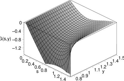
Figure 3: Plots of the gravity profile $G(s,y)=g_{B}\,\alpha^{\prime}$, for the specific case of $s>s_{r}$ (left plot), and $s<s_{r}$ (right plot), respectively. For the first case, $s>s_{r}$, the gravity profile takes negative values, reflecting a repulsive character, in the range $0<y<y_{m}=\sqrt{2}$. For the second case, $s<s_{r}$ we have used $s=0.5$. The gravity profile is given by the dashed curves, and is negative in the range $y<y_{1}$, where $f>0$. The dashed curves represent the gravity profile, and the solid line depicts $f(s,y)$.

The surface stresses of the thin shell are provided by

$$\sigma = -\frac{1}{4\pi a_{0}}\left[\sqrt{1-\frac{2M}{a_{0}}}-\sqrt{1-\frac{2g_{B}a_{0}^{2}}{s(a_{0}^{2}+g_{B}^{2})^{3/2}}}\,\right],$$ (52)

$${\cal P} = \frac{1}{8\pi a_{0}}\left\{\frac{1-\frac{M}{a_{0}}}{\sqrt{1-\frac{2M}{a_{0}}}}-\frac{1-\frac{g_{B}a_{0}^{2}(a_{0}^{2}+4g_{B}^{2})}{s(a_{0}^{2}+g_{B}^{2})^{5/2}}}{\sqrt{1-\frac{2g_{B}a_{0}^{2}}{s(a_{0}^{2}+g_{B}^{2})^{3/2}}}\,}\right\}$$ (53)

The total mass of the Bardeen gravastar is given by

$$M={\frac{ga_{0}^{3}}{s\left({a_{0}}^{2}+{g}^{2}\right)^{3/2}}}+m_{s}(a_{0})\left[\sqrt{1-{\frac{2ga_{0}^{2}}{s\left({a_{0}}^{2}+{g}^{2}\right)^{3/2}}}}-\frac{m_{s}(a_{0})}{2a_{0}}\right]\,.$$ (54)

4 Dual $P$ formalism

Despite of the fact that nonlinear electrodynamics may be represented in terms of a nonlinear electrodynamic field, $F_{\mu\nu}$, and its invariants, one may introduce a dual representation in terms of an auxiliary field $P_{\mu\nu}$. The introduction of $P_{\mu\nu}$, proved to be extremely useful in the derivation of exact solutions in general relativity, especially in the electric regime. The dual representation of nonlinear electrodynamics is obtained by a Legendre transformation given by

$$H=2FL_{F}-L\,.$$ (55)

The structural function $H$ is a function of a factor $P$, defined by $P=P_{\mu\nu}P^{\mu\nu}/4$. In this representation, the theory is reformulated in terms of the structural function $H$ by the following relationships

$$P_{\mu\nu}=L_{F}F_{\mu\nu}\,,\qquad F_{\mu\nu}=H_{P}P_{\mu\nu}\,,$$ (56)

$$L=2PH_{P}-H\,,\qquad L_{F}H_{P}=1\,,$$ (57)

where $H_{P}=dH/dP$. The invariant $P$ is given by

$$P=\frac{1}{4}\,P_{\mu\nu}P^{\mu\nu}=-\frac{1}{2}\left(P_{tr}^{2}-\frac{1}{r^{4}\sin^{2}\theta}\,P_{\theta\phi}^{2}\right)$$ (58)

The stress-energy tensor in the dual $P$ formalism is written as

$$T_{\mu\nu}=g_{\mu\nu}\,(2PH_{P}-H)-P_{\mu\alpha}P_{\nu}{}^{\alpha}\,H_{P}\,,$$ (59)

and in the orthonormal reference frame, provides the following components

$$T_{\hat{t}\hat{t}} = -T_{\hat{r}\hat{r}}=H-\frac{1}{r^{4}\sin^{2}\theta}\,P_{\theta\phi}^{2}\,H_{P}\,,$$ (60)

$$T_{\hat{\phi}\hat{\phi}} = T_{\hat{\theta}\hat{\theta}}=-H-P_{tr}^{2}\,H_{P}\,.$$ (61)

The electromagnetic field equations in the $P$ dual form are the following

$$P^{\mu\nu}{}_{;\mu}=0\;,\qquad\left(H_{P}\,^{*}P^{\mu\nu}\right)_{;\mu}=0\,.$$ (62)

We emphasize that the tensor $F_{\mu\nu}=H_{P}\,P_{\mu\nu}$ is the physically relevant quantity. However, one may obtain electric solutions easier by considering the $P$ dual formalism.

4.1 Electric field

Equation (55) implies that for the pure electric field, $B=0$, together with equations (27)-(29) provide the following extremely useful and simplified relationship

$$H_{E}=\frac{1}{4\pi}\frac{m^{\prime}}{r^{2}}\,,$$ (63)

where $H_{E}$ is the $H$ structural function for this case and the correspondent $P$ invariant

$$P_{E}=-\frac{q_{e}^{2}}{2r^{4}}\,.$$ (64)

Thus, using the dual $P$ formalism, it is easier to find nonlinear electrodynamic solutions than in the $F$ formalism, for the specific case of pure electric fields. We consider several solutions in this section.

4.1.1 Ayón-Beato$-$Garcia gravastar.

In this section, we are interested in constructing a specific gravastar geometry from a regular black hole solution coupled to nonlinear electrodynamics, found by Ayón-Beato$-$Garcia [21]. Although this solution is indeed regular, i.e., the metric, curvature invariants and the electric field are regular everywhere, one still verifies the presence of event horizons, and consequently the associated difficulties related to these null hypersurfaces. Consider the specific Ayón-Beato$-$Garcia structural function [21] given in the following form

$$H=\frac{-P}{4\pi\cosh^{2}\left(s\sqrt[4]{-2q_{e}^{2}P}\;\right)}\,,$$ (65)

where $s$ is an adimensional constant. Note that $H$ assumes the Einstein-Maxwell form in the weak field limit, i..e, $H\approx-P/4\pi$ for $P\ll 1$. We also have

$$H_{P}=\frac{1}{8\pi\cosh^{2}\left(s\sqrt[4]{-2q_{e}^{2}P}\;\right)}\;\left[s\,\tanh^{2}\left(s\sqrt[4]{-2q_{e}^{2}P}\;\right)-2\right]\,.$$ (66)

Using equation (64), $H$ and $H_{P}$ may be recast as

$$H=\frac{q^{2}}{8\pi r^{4}\cosh^{2}\left(\frac{sq}{r}\right)}\,,\qquad H_{P}=\frac{1}{8\pi\cosh^{2}\left(\frac{sq}{r}\right)}\;\left[\left(\frac{sq}{r}\right)\,\tanh^{2}\left(\frac{sq}{r}\right)-2\right]\,,$$ (67)

where the definition $q=|q_{e}|$ is used.

The mass function is determined by using equation (63), and is given by

$$m(r)=\frac{q}{2s}\left[1-\tanh\left(\frac{sq}{r}\right)\right]\,.$$ (68)

With this solution at hand, the energy density and the principal pressures take the following form

$$\rho = -p_{r}=\frac{q^{2}}{8\pi r^{4}}\left[1-\tanh^{2}\left(\frac{sq}{r}\right)\right]\,,$$ (69)

$$p_{t} = -\frac{q^{2}}{8\pi r^{4}}\left[1-\tanh^{2}\left(\frac{sq}{r}\right)\right]\,\left[\left(\frac{sq}{r}\right)\tanh\left(\frac{sq}{r}\right)-1\right]\,.$$ (70)

Analysing the geometry of the solution, consider the metric fields

$$e^{2\alpha(r)}=e^{-2\beta(r)}=1-\frac{q}{s\,r}\left[1-\tanh\left(\frac{sq}{r}\right)\right]\,.$$ (71)

Defining $y=r/(sq)$, the above equation takes the form

$$f(s,y)=1-\frac{\left[1-\tanh\left(1/y\right)\right]}{s^{2}y}\,.$$ (72)

Using $\partial f/\partial y=0$, which may be re-expressed as $[1-\tanh(1/y)][y-1-\tanh(1/y)]=0$, we verify that $f$ possesses a single minimum, $y_{m}\approx 1.564$, independently of the value of $s$. Now, $f(s,y_{m})=0$ has a single positive root at $s\approx 0.5277$. However, for this case, we have $f(s,y)>0$ if $s>s_{r}$. If $s<s_{r}$, then $f(s,y)$ possesses two roots, $y_{1}$ and $y_{2}$, which reflects the existence of event horizons.

We also need to verify the WEC, given by $m^{\prime}\geq 0$ and $N\geq 0$, which taking into account the definition $y=r/(sq)$, assume the following form

$$m^{\prime}(s,y) = \frac{1}{2s^{2}y^{2}}\left[1-\tanh^{2}\left(\frac{1}{y}\right)\right]\,,$$ (73)

$$N(s,y) = \frac{1}{s^{2}y^{2}}\left[1-\tanh^{2}\left(\frac{1}{y}\right)\right]\,\left[2-\left(\frac{1}{y}\right)\tanh\left(\frac{1}{y}\right)\right]\,,$$ (74)

which are represented in figure 4. Note that at the center $y=r=0$, the factor $N$ becomes zero, showing that $p_{r}=p_{t}$, as was to be expected. We have only considered the range $0.3<s<1$, for representational convenience. Note that $m^{\prime}\geq 0$ is verified for all values of $s$ and $y$. However, $N$ is negative in the range $0<y<y_{N}\simeq 0.4842$, for all values of $s$. Thus the WEC is violated in the range $0<y<y_{N}\simeq 0.4842$.

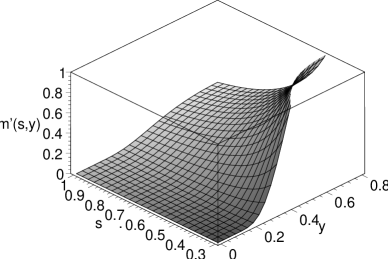
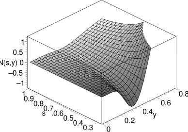
Figure 4: Plots of the WEC, $m^{\prime}(r)$ and $N(r)$, respectively. We have only plotted the range $0.3<s<1$, for representational convenience. $m^{\prime}\geq 0$ is verified for all values of $s$ and $y$. However, $N$ is negative in the range $0<y<y_{N}\simeq 0.4842$, for all values of $s$.

For the gravity profile we deduce the following relationship

$$\alpha^{\prime}=\frac{\left\{1-\tanh\left(\frac{sq}{r}\right)-\left(\frac{sq}{r}\right)\left[1-\tanh^{2}\left(\frac{sq}{r}\right)\right]\right\}}{2r\left[\frac{sr}{q}-1+\tanh\left(\frac{sq}{r}\right)\right]}\,,$$ (75)

which using the definition $y=r/(sq)$, takes the form

$$G=(2sq)\alpha^{\prime}=\frac{\left\{1-\tanh\left(\frac{1}{y}\right)-\left(\frac{1}{y}\right)\left[1-\tanh^{2}\left(\frac{1}{y}\right)\right]\right\}}{y\left[s^{2}y-1+\tanh\left(\frac{1}{y}\right)\right]}\,.$$ (76)

The case of $s>s_{r}$, and for which $\alpha^{\prime}<0$, is plotted in figure 5. Note that the gravity profile takes negative values, reflecting a repulsive character, in the range $0<y<y_{m}$ for $s>s_{r}$. Thus, one may match this interior solution at $r_{m}=sqy_{m}>a_{0}>2M$. For the case of $s<s_{r}$ and for $f>0$, the gravity profile is only negative for $y<y_{1}$, being positive for $y>y_{2}$. Note that the gravity profile has asymptotes precisely at the roots of $f$. Thus, one may match this solution at $r_{1}=sqy_{1}>a_{0}>2M$, to an exterior Schwarzschild spacetime.

Figure 5: Plots of the gravity profile $G=(2sq)\alpha^{\prime}$, for the specific case of $s>s_{r}$ (left plot), and $s<s_{r}$ (right plot), respectively. For the latter we have used $s=0.4277$. The gravity profile is given by the dashed curves. For the first case, $s>s_{r}$, the gravity profile takes negative values, reflecting a repulsive character, in the range $0<y<y_{m}\simeq 1.564$. For the case of $s<s_{r}$ and for $f>0$, the gravity profile is only negative for $y<y_{1}$.

Then, with our solution for the mass function, alongside $H$ and $H_{P}$, we can cast the following relevant functions for the system

$$E(r)=-\frac{q}{8\pi r^{2}}\left[1-\tanh^{2}\left(\frac{sq}{r}\right)\right]\left[2-\left(\frac{sq}{r}\right)\tanh\left(\frac{sq}{r}\right)\right]\,,$$ (77)

$$F=-\frac{1}{2}\left\{\frac{q}{8\pi r^{2}}\left[1-\tanh^{2}\left(\frac{sq}{r}\right)\right]\left[2-\left(\frac{sq}{r}\right)\tanh\left(\frac{sq}{r}\right)\right]\right\}^{2}\,,$$ (78)

$$L_{F}=-8\pi\left\{\left[1-\tanh^{2}\left(\frac{sq}{r}\right)\right]\left[2-\left(\frac{sq}{r}\right)\tanh\left(\frac{sq}{r}\right)\right]\right\}^{-1}$$ (79)

$$L=-\frac{q^{2}}{8\pi r^{4}}\left[1-\tanh^{2}\left(\frac{sq}{r}\right)\right]\left[\left(\frac{sq}{r}\right)\tanh\left(\frac{sq}{r}\right)-1\right]\,,$$ (80)

$$2FL_{F}=\frac{q^{2}}{8\pi r^{4}}\left[1-\tanh^{2}\left(\frac{sq^{2}}{r^{2}}\right)\right]\left[2-\left(\frac{sq}{r}\right)\tanh\left(\frac{sq}{r}\right)\right]\,.$$ (81)

Given this, the above interior Ayón-Beato$-$Garcia spacetime may be matched to an exterior Schwarzschild solution, at the junction interface, $a_{0}$, with the surface stresses given by

$$\sigma = -\frac{1}{4\pi a_{0}}\left(\sqrt{1-\frac{2M}{a_{0}}}-\sqrt{1-\frac{q}{sa_{0}}\left[1-\tanh\left(\frac{sq}{a_{0}}\right)\right]}\,\right),$$ (82)

$${\cal P} = \frac{1}{8\pi a_{0}}\left[\frac{1-\frac{M}{a_{0}}}{\sqrt{1-\frac{2M}{a_{0}}}}-\frac{1-\left(\frac{q}{2sa_{0}}\right)\left\{1-\tanh\left(\frac{sq}{a_{0}}\right)+\left(\frac{sq}{a_{0}}\right)\left[1-\tanh^{2}\left(\frac{sq}{a_{0}}\right)\right]\right\}}{\sqrt{1-\frac{q}{sa_{0}}\left[1-\tanh\left(\frac{sq}{a_{0}}\right)\right]}}\,\right]\,.$$ (83)

The total mass of the gravastar is given by

$$M=\left(\frac{q}{2s}\right)\left[1-\tanh\left(\frac{sq}{a_{0}}\right)\right]+m_{s}(a_{0})\left\{\sqrt{1-\frac{q}{sa_{0}}\left[1-\tanh\left(\frac{sq}{a_{0}}\right)\right]}-\frac{m_{s}(a_{0})}{2a_{0}}\right\}\,,$$ (84)

where $m_{s}(a_{0})$ is the surface mass of the thin shell, given by $m_{s}(a_{0})=4\pi a_{0}^{2}\sigma$.

Summarizing the above results, we have the following: $(i)$ For $s>s_{r}$, the factor $f$ is positive for all values of $y$, proving the absence of event horizons. However, the gravity profile, $\alpha^{\prime}$, is only negative in the range $0<y<y_{m}$, reflecting a repulsive character of the geometry, which is essential for gravastar solutions. Finally, the WEC is satisfied only in the range $y\geq y_{N}$, for all values of $s$. Thus, in conclusion, one may match this interior Ayón-Beato$-$Garcia geometry to an exterior Schwarzschild solution, at $r_{m}=sqy_{m}>a_{0}>2M$, whilst the WEC is violated in the range $0<y<y_{N}<y_{m}$. $(ii)$ For $s<s_{r}$, the factor $f$ has two roots, $y_{1}$ and $y_{2}$. $f(s,y)$ is positive for $y<y_{1}$ and $y>y_{2}$, while the gravity profile is only negative in the range $y<y_{1}$. As for the previous case, the WEC is violated in the range $y<y_{N}<y_{1}$, as $N<0$. Therefore, to construct a gravastar geometry, one needs to match the Ayón-Beato$-$Garcia solution to an exterior Schwarzschild spacetime at $r_{1}=sqy_{1}>a_{0}>2M$, with the consequent violation of the WEC in the range $0<y<y_{N}<y_{1}$. Another important characteristic that both cases exhibit is an electrically superconductive behavior, at the center, as $L_{F}\rightarrow\infty$ as $r\rightarrow 0$.

One may also consider other regular black hole solutions obtained by Ayón-Beato$-$Garcia, in particular the structural functions given in Refs. [20, 22], however, we shall not endeavor in this analysis. The message that one may extract, is that one may, in principle, construct a wide variety of gravastar models in the context of nonlinear electrodynamics, by using the regular black hole solutions found by Ayón-Beato$-$Garcia [20, 21, 22].

4.1.2 Nonlinear modified Tolman-Matese-Whitman mass function.

Consider the following structural function and its derivative given by

$$H=\frac{\sqrt{-2P}(1+3\alpha\,\sqrt{-2P}\,)}{\alpha(1+\alpha\,\sqrt{-2P})^{2}}\,,\qquad H_{P}=-\frac{(1+5\alpha\,\sqrt{-2P}\,)}{\alpha\sqrt{-2P}(1+\alpha\,\sqrt{-2P})^{3}}\,.$$ (85)

Note, however, that this structural function does not assume the Einstein-Maxwell form in the weak field limit, i..e, $H\approx(-P)^{1/2}$ for $P\ll 1$. However, as mentioned above, we are not preoccupied with regaining the weak field limit in the specified range $0\leq r\leq a$, as the interior nonlinear electrodynamic solution is matched at a junction interface $a$, to an exterior vacuum geometry.

Taking into account $P=-q_{e}^{2}/(2r^{4})$, $H$ and $H_{P}$ take the form

$$H=\frac{3+\frac{r^{2}}{\alpha q}}{\alpha^{2}\left(1+\frac{r^{2}}{\alpha q}\right)^{2}}\,,\qquad H_{P}=-\frac{\left(\frac{r^{2}}{\alpha q}\right)^{3}\left(5+\frac{r^{2}}{\alpha q}\right)}{\left(1+\frac{r^{2}}{\alpha q}\right)^{3}}\,,$$ (86)

where the definition $q=|q_{e}|$ is used. The mass function may be integrated to yield

$$m(r)=\frac{4\pi r^{3}}{\alpha^{2}\left(1+\frac{r^{2}}{\alpha q}\right)}\,.$$ (87)

Note that this mass function is similar in form to the Tolman-Matese-Whitman function analyzed in detail in Ref. [11], which represents a monotonic decreasing energy density in the gravastar interior, and was used previously in the analysis of isotropic fluid spheres by Matese and Whitman [34]. Thus, we denote the mass function given by equation (87) the nonlinear modified Tolman-Matese-Whitman mass function.

The stress-energy tensor components take the following form

$$\rho=-p_{r}={\frac{q\left(3\alpha q+{r}^{2}\right)}{\alpha\left(\alpha q+{r}^{2}\right)^{2}}}\;,\qquad p_{t}=-{\frac{{q}^{2}\left(3\alpha q-{r}^{2}\right)}{\left(\alpha q+{r}^{2}\right)^{3}}}\,.$$ (88)

The WEC is also satisfied as the following factors

$$m^{\prime}(r)={\frac{4\pi{r}^{2}q\left(3\alpha q+{r}^{2}\right)}{\alpha\left(\alpha q+{r}^{2}\right)^{2}}}\;,\qquad N(r)={\frac{8\pi{r}^{4}q\left(5\alpha q+{r}^{2}\right)}{\alpha\left(\alpha q+{r}^{2}\right)^{3}}}\;,$$ (89)

are manifestly positive. Note that at the center, $r=0$, we have $N=0$, so that $p_{r}=p_{t}$, as was to be expected.

Analysing the geometry of the solution, consider

$$e^{2\alpha(r)}=e^{-2\beta(r)}=1-\frac{8\pi r^{2}}{\alpha^{2}\left(1+\frac{r^{2}}{\alpha q}\right)}\,,$$ (90)

Defining $s^{2}=8\pi q/\alpha$ and $y^{2}=r^{2}/(\alpha q)$, so that the above equation takes the form

$$f(s,y)=1-\frac{s^{2}y^{2}}{1+y^{2}}\,.$$ (91)

Note the absence of event horizons for $s<1$. If $s>1$, then $f$ possesses a positive root situated at $y_{r}=1/\sqrt{s^{2}-1}$.

The gravity profile is given by

$$\alpha^{\prime}=-{\frac{8\pi\alpha{q}^{2}r}{\left({\alpha}^{2}q+\alpha{r}^{2}-8\pi{r}^{2}q\right)\left(\alpha q+{r}^{2}\right)}}\;.$$ (92)

which using the definitions $s^{2}=8\pi q/\alpha$ and $y^{2}=r^{2}/(\alpha q)$, takes the following form

$$G=\sqrt{\alpha q}\;\alpha^{\prime}=-\frac{s^{2}y}{\left[1+(1-s^{2})y^{2}\right](1+y^{2})}\;.$$ (93)

One readily verifies that $\alpha^{\prime}<$ for $s\leq 1$. For $s\geq 1$, we also verify that $\alpha^{\prime}<0$ for $y<y_{r}$. See figure 6 for the latter case, with the specific choice of $s=1.1$. An asymptote of $\alpha^{\prime}$ exists precisely at the root.

Figure 6: Plot of the gravity profile $G=\sqrt{\alpha q}\;\alpha^{\prime}$, for the specific case of $s>s_{r}$. We have used $s=1.1$. The gravity profile takes negative values, reflecting a repulsive character, in the range $0<y<y_{r}$.

The electric field and the $F$ invariant are given by

$$E(r)=-{\frac{{r}^{4}\left(5\alpha q+{r}^{2}\right)}{\alpha\,\left(\alpha q+{r}^{2}\right)^{3}}}\,,\qquad F=-\frac{1}{2}\left[{\frac{{r}^{4}\left(5\alpha q+{r}^{2}\right)}{\alpha\left(\alpha q+{r}^{2}\right)^{3}}}\right]^{2}\,,$$ (94)

respectively. We also have the following relationships

$$L=-{\frac{{q}^{2}\left(3\alpha q-{r}^{2}\right)}{\left(\alpha q+{r}^{2}\right)^{3}}}\;,\qquad L_{F}=-{\frac{q\alpha\left(\alpha q+{r}^{2}\right)^{3}}{{r}^{6}\left(5\alpha q+{r}^{2}\right)}}\,,$$ (95)

In summary, one may match the interior solution to an exterior Schwarzschild spacetime, at a junction interface, $a_{0}>2M$. If $s>1$, then the matching needs to be done at $r_{r}=\sqrt{\alpha q}\,y_{r}>a_{0}>2M$. The surface stresses are given by

$$\sigma = -\frac{1}{4\pi a_{0}}\left\{\sqrt{1-\frac{2M}{a_{0}}}-\sqrt{1-\frac{8\pi a_{0}^{2}}{\alpha^{2}\left(1+\frac{a_{0}^{2}}{\alpha q}\right)}}\,\right\},$$ (96)

$${\cal P} = \frac{1}{8\pi a_{0}}\left\{\frac{1-\frac{M}{a_{0}}}{\sqrt{1-\frac{2M}{a_{0}}}}-\left[1-\frac{8\pi a_{0}^{2}\left(2+\frac{a_{0}^{2}}{\alpha q}\right)}{\alpha^{2}\left(1+\frac{a_{0}^{2}}{\alpha q}\right)^{2}}\right]\Bigg{/}\sqrt{1-\frac{8\pi a_{0}^{2}}{\alpha^{2}\left(1+\frac{a_{0}^{2}}{\alpha q}\right)}}\,\right\}\,.$$ (97)

The total mass of the gravastar is given by

$$M=\frac{4\pi a_{0}^{3}}{\alpha^{2}\left(1+\frac{a_{0}^{2}}{\alpha q}\right)}+m_{s}(a_{0})\left\{\sqrt{1-\frac{8\pi a_{0}^{2}}{\alpha^{2}\left(1+\frac{a_{0}^{2}}{\alpha q}\right)}}-\frac{m_{s}(a_{0})}{2a_{0}}\right\}\,,$$ (98)

where $m_{s}(a_{0})$ is the surface mass of the thin shell, given by $m_{s}(a_{0})=4\pi a_{0}^{2}\sigma$.

4.2 Magnetic field

Now for the $E=0$ case, equations (30)-(32) together with (55) provide the following relationships

$$H_{B}=\frac{1}{8\pi}\frac{m^{\prime\prime}}{r}\,,$$ (99)

where $H_{B}$ is the $H$ structural function for this case and the correspondent $P$ invariant is given by

$$P_{B}=\frac{N^{2}}{2(8\pi q_{m})^{2}}\,.$$ (100)

We can, in principle, find new solutions for the mass function $m(r)$ by choosing a suitable form of the $H=H_{B}$ structural function. Although this treatment is far from being trivial, we have considered the $F$ formalism to find purely magnetic solutions.

5 Summary and duscussion

Gravastar models have recently been proposed as an alternative to black holes, mainly to avoid the associated difficulties with event horizons and singularities. In this work, we have been interested in the construction of gravastar models coupled to nonlinear electrodynamics. Using the $F$ representation, we have considered specific forms of Lagrangians describing magnetic gravastars, which may be interpreted as self-gravitating magnetic monopoles with a charge $g$. Using the $P$ formulation of nonlinear electrodynamics, it is easier to find electric solutions, and considering specific structural functions we further explored the characteristics and physical properties of these solutions. We have matched these interior nonlinear electrodynamic geometries to an exterior Schwarzschild spacetime at a junction interface $a$, thus avoiding the problematic issues related to the singularities and event horizons. We emphasize that what is required from a spherically symmetric solution of the Einstein equations to be a gravastar model, is the presence of a repulsive nature of the interior solution, which is characterized by the notion of the “gravity profile”. It is important to point out that to be a nonlinear electrodynamic model, the Maxwellian limit, $L\sim-F$ and $L_{F}\sim-1$, has to be recovered in the weak field limit, $F\ll 1$. For the spacetimes considered in this work, it is only at $r\rightarrow\infty$ that the weak field limit, $F\rightarrow 0$, is recovered. Therefore, in the gravastar models that we construct, it is not necessary to regain the weak field limit in the specified range $0\leq r\leq a$ of the interior nonlinear electrodynamic solution. Thus, we have used general Lagrangians and structural functions that are strongly non-Maxwellian in the weak field limit, namely the Bardeen and the Tolman-Matese-Whitman solutions. In conclusion, a rather wide variety of gravastar solutions may be constructed within the context of nonlinear electrodynamics.

References

References

- [1] G. Chapline, E. Hohlfeld, R. B. Laughlin and D. I. Santiago, “Quantum Phase Transitions and the Breakdown of Classical General Relativity,” Int. J. Mod. Phys. A 18 3587-3590 (2003) [arXiv:gr-qc/0012094].
- [2] P. O. Mazur and E. Mottola, “Gravitational Condensate Stars: An Alternative to Black Holes,” [arXiv:gr-qc/0109035]; P. O. Mazur and E. Mottola, “Dark energy and condensate stars: Casimir energy in the large,” Proceedings of the Sixth Workshop on Quantum Field Theory Under the Influence of External Conditions, [arXiv:gr-qc/0405111]; P. O. Mazur and E. Mottola, “Gravitational Vacuum Condensate Stars,” Proc. Nat. Acad. Sci. 111, 9545 (2004) [arXiv:gr-qc/0407075].
- [3] G. Chapline, “Dark energy stars,” Proceedings of the 22nd Texas Conference on Relativistic Astrophysics, California (2004), [arXiv:astro-ph/0503200].
- [4] R. Doran, F. S. N. Lobo and P. Crawford, “Interior of a Schwarzschild black hole revisited,” [arXiv:gr-qc/0609042].
- [5] M. A. Abramowicz, W. Kluzniak and J. P. Lasota, “No observational proof of the black-hole event-horizon,” Astron. Astrophys. 396 L31 (2002) [arXiv:astro-ph/0207270].
- [6] I. Dymnikova, “Vacuum nonsingular black hole,” Gen. Rel. Grav. 24, 235 (1992); I. Dymnikova, “The algebraic structure of a cosmological term in spherically symmetric solutions,” Phys. Lett. B472, 33-38 (2000) [arXiv:gr-qc/9912116]; I. Dymnikova, “Cosmological term as a source of mass,” Class. Quant. Grav. 19 725-740 (2002) [arXiv:gr-qc/0112052]; I. Dymnikova, “Spherically symmetric space-time with the regular de Sitter center,” Int. J. Mod. Phys. D 12, 1015-1034 (2003) [arXiv:gr-qc/0304110];
- [7] M. Visser and D. L. Wiltshire, “Stable gravastars - an alternative to black holes?,” Class. Quant. Grav. 21 1135-1152 (2004) [arXiv:gr-qc/0310107].
- [8] B. M. N. Carter, “Stable gravastars with generalised exteriors,” Class. Quant. Grav. 22 4551-4562 (2005) [arXiv:gr-qc/0509087].
- [9] C. Cattoen, T. Faber and M. Visser, “Gravastars must have anisotropic pressures,” Class. Quant. Grav. 22 4189-4202 (2006) [arXiv:gr-qc/0505137].
- [10] A. DeBenedictis, D. Horvat, S. Ilijic, S. Kloster and K. S. Viswanathan, “Gravastar Solutions with Continuous Pressures and Equation of State,” Class. Quant. Grav. 23 2303-2316 (2006) [arXiv:gr-qc/0511097].
- [11] F. S. N. Lobo, “Stable dark energy stars,” Class. Quant. Grav. 23, 1525 (2006) [arXiv:astro-ph/0508115].
- [12] S. Sushkov, “Wormholes supported by a phantom energy,” Phys. Rev. D 71, 043520 (2005) [arXiv:gr-qc/0502084]; F. S. N. Lobo, “Phantom energy traversable wormholes,” Phys. Rev. D 71, 084011 (2005) [arXiv:gr-qc/0502099]; F. S. N. Lobo, “Stability of phantom wormholes,” Phys. Rev. D 71, 124022 (2005) [arXiv:gr-qc/0506001].
- [13] N. Bilić, G. B. Tupper and R. D. Viollier, “Born-Infeld phantom gravastars,” JCAP 0602, 013 (2006) [arXiv:astro-ph/0503427].
- [14] N. Seiberg and E. Witten, “String theory and noncommutative geometry,” JHEP 9909, 032 (1999) [arXiv:hep-th/9908142].
- [15] M. Novello, S. E. P. Bergliaffa and J. Salim, “Nonlinear electrodynamics and the acceleration of the universe,” Phys. Rev. D 69 127301 (2004) [arXiv:astro-ph/0312093]; R. Garcia-Salcedo and N. Breton, “Born-Infeld Cosmologies,” Int. J. Mod. Phys. A15, 4341-4354 (2000) [arXiv:gr-qc/0004017]; R. Garcia-Salcedo and N. Breton, “Nonlinear electrodynamics in Bianchi spacetimes,” Class. Quant. Grav. 20, 5425-5437 (2003) [arXiv:hep-th/0212130]; R. Garcia-Salcedo and N. Breton, “Singularity-free Bianchi spaces with nonlinear electrodynamics,” Class. Quant. Grav. 22, 4783-4802 (2005) [arXiv:gr-qc/0410142]; D. N. Vollick, “Anisotropic Born-Infeld Cosmologies,” Gen. Rel. Grav. 35, 1511-1516 (2003) [arXiv:hep-th/0102187].
- [16] A. V. B. Arellano and F. S. N. Lobo, “Evolving wormhole geometries within nonlinear electrodynamics,” Class. Quant. Grav. 23 5811-5824 (2006) [arXiv:gr-qc/0608003].
- [17] A. V. B. Arellano and F. S. N. Lobo, “Non-existence of static, spherically symmetric and stationary, axisymmetric traversable wormholes coupled to nonlinear electrodynamics,” Class. Quant. Grav. 23 7229-7244 (2006) [arXiv:gr-qc/0604095].
- [18] M. Born, “On the quantum theory of the electromagnetic field,” Proc. Roy. Soc. Lond. A143, 410 (1934); M. Born and L. Infeld, “Foundations of the new field theory,” Proc. Roy. Soc. A144, 425 (1934).
- [19] J. F. Plebański, “Lectures on non-linear electrodynamics,” monograph of the Niels Bohr Institute Nordita, Copenhagen (1968). S. A. Gutiérrez, A. L. Dudley and J. F. Plebański, “Signals and discontinuities in general relativistic nonlinear electrodynamics,” J. Math. Phys. 22, 2835 (1981).
- [20] E. Ayón-Beato and A. García, “Regular black hole in general relativity coupled to nonlinear electrodynamics,” Phys. Rev. Lett. 80, 5056-5059 (1998) [arXiv:gr-gc/9911046].
- [21] E. Ayón-Beato and A. García, “New regular black hole solution from non-linear electrodynamics,” Phys. Lett. B 464, 25 (1999) [arXiv:hep-th/9911174];
- [22] E. Ayón-Beato and A. García, “Non-singular charged black hole solutions for non-linear source,” Gen. Rel. Grav. 31, 629-633 (1999) [arXiv:gr-gc/9911084].
- [23] K. A. Bronnikov, “Regular magnetic black holes and monopoles from nonlinear electrodynamics,” Phys. Rev. D 63, 044005 (2001) [arXiv:gr-qc/0006014].
- [24] A. Burinskii and S. R. Hildebrandt, “New type of regular black holes and particlelike solutions from nonlinear electrodynamics,” Phys. Rev. D 65, 104017 (2002) [arXiv:hep-th/0202066].
- [25] I. Dymnikova, “Regular electrically charged structures in Nonlinear Electrodynamics coupled to General Relativity,” Class. Quant. Grav. 21, 4417-4429 (2004) [arXiv:gr-qc/0407072].
- [26] F. S. N. Lobo, “Van der Waals quintessence stars,” to appear in Phys. Rev. D, [arXiv:gr-qc/0610118].
- [27] J. P. S. Lemos, F. S. N. Lobo and S. Q. de Oliveira, “Morris-Thorne wormholes with a cosmological constant,” Phys. Rev. D 68, 064004 (2003) [arXiv:gr-qc/0302049]; F. S. N. Lobo, “Surface stresses on a thin shell surrounding a traversable wormhole,” Class. Quant. Grav. 21 4811 (2004) [arXiv:gr-qc/0409018]; F. S. N. Lobo, “Energy conditions, traversable wormholes and dust shells,” Gen. Rel. Grav. 37, 2023 (2005) [arXiv:gr-qc/0410087]; F. S. N. Lobo and P. Crawford, “Stability analysis of dynamic thin shells,” Class. Quant. Grav. 22, 4869 (2005), [arXiv:gr-qc/0507063].
- [28] H. A. Buchdahl, “General Relativistic Fluid Spheres,” Phys. Rev. 116, 1027 (1959).
- [29] B. V. Ivanov, “Maximum bounds on the surface redshift of anisotropic stars,” Phys. Rev. D 65, 104011 (2002) [arXiv:gr-qc/0203070].
- [30] N. Breton, “Stability of nonlinear magnetic black holes,” Phys. Rev. D 72, 044015 (2005) [arXiv:hep-th/0502217].
- [31] J. Bardeen, presented at GR5, Tiflis, U.S.S.R., and published in the conference proceedings (1968).
- [32] E. Ayón-Beato and A. García, “The Bardeen Model as a Nonlinear Magnetic Monopole,” Phys. Lett. B493 149-152 (2000) [arXiv:gr-gc/0009077].
- [33] J. P. S. Lemos and V. T. Zanchin, “Gravitational magnetic monopoles and Majumdar-Papapetrou stars,” J. Math. Phys. 47 042504 (2006) [arXiv:gr-qc/0603101].
- [34] J. J. Matese and P. G. Whitman, “New methods for extracting equilibrium configurations in general relativity,” Phys. Rev. D 22 1270-1275 (1980).