The two body problem : analytical results in a toy model of relativistic gravity

Abstract

The two body problem in a scalar theory of gravity is investigated. We focus on the closest theory to General Relativity (GR), namely Nordström’s theory of gravity ($1913$). The gravitational field can be exactly solved for any configuration of point-particles. We then derive the exact equations of motion of two inspiraling bodies including the exact self-forces terms. We prove that there is no innermost circular orbit (ICO) in the exact theory whereas we find (order-dependent) ICOs if post-Newtonian (PN) truncations are used. We construct a solution of the two body problem in an iterative (non-PN) way, which can be viewed as a series in powers of $(v/c)^{5}$. Besides this rapid convergence, each order also provides non-perturbative information. Starting from a circular Newtonian-like orbit, the first iteration already yields the 4.5 PN radiation reaction. These results not only shed light on some non-perturbative effects of relativistic gravity, but may also be useful to test numerical codes.

1 Introduction

The two-body problem in GR is both an important and difficult issue. Various approach have been investigated. One generically needs some assumptions and simulations (numerical relativity) or perturbatives techniques (PN expansion, e.g Templatesa3PN ). In both cases it remains difficult to quantify the errors one makes. This point is however crucial in order to interpret the coming-soon data.

It should thus be very interesting to test the numerical codes and the assumptions usually made in the two-body problem within a toy model of GR. One may also hope that some generic non-perturbative effects may be found, that could also occur in GR. This toy model should be simple enough to treat analytically (at least partially) the two body problem, but should also be as close as possible to GR. Metric scalar theories of gravity are perfect candidates of such toy models.

This idea is not a new one. It has already been used in order to test numerical codes, see e.g Gravscalaire1 ; Gravscalaire2 or, more recently, the validity of the Quasi Equilibrium (QE) scheme GravscalaireQE . However we wish here to focus on a particular theory of this class (namely Nordström’s one), which is, to our mind, the best motivated toy-model of GR, and which has not been used in the literature. An important point is that Nordström’s theory respects the Strong Equivalence Principle (SEP) and thus enables us to consider constant-mass points-particles, whereas this cannot be justified in others models considered in the literature. We also want to go further in the analytical resolution of the two-body problem, by using one of the great advantages of Nordström’s theory: the linearity of the field equation.

In Section II we recall the basic features of such metric scalar theories and notably the particular case of Nordström’s theory. In Section III, we solve exactly the metric in terms of $N$ arbitrary massive point particles. We then derive the exact equations of motion of such bodies which notably involve finite self-force terms.

In Section IV, we restrict to the equal-mass two-body case and investigate the circular motion. We derive the analytical relation between the radius and the orbital velocity. We compute the exact energy of the binary in such a circular configuration and show that the theory does not exhibit an innermost circular orbit (ICO), whereas such ICOs are found if one works with PN truncations of the exact energy.

In Section V, starting from this circular solution, we show that the inspiral motion can be found order by order in power of $(v/c)^{5}$, where $v$ is the velocity of the bodies. This behavior is directly related to the leading multipolar emission of the system, namely the quadrupolar one. Furthermore, this expansion is not a PN one since each orders yield non-perturbative information on the motion.

In Section VI, we show some analytical and numerical results. We give the exact rate of change of the velocity up to 4.5 PN and the radius up to 7PN. We also plot these two quantities and by numerical integration, we plot the corresponding inspiral motion. This paper is a short version of the self-contained article NotreArticle in which more technical details can be found.

2 A quick look at Nordström’s theory of gravity

We first introduce briefly metric scalar theories of gravity. The action reads

$$\mathcal{S}=-\frac{c^{4}}{8\pi G}\int\sqrt{-\eta}\frac{d^{4}x}{c}\eta^{\mu\nu}\partial_{\mu}\varphi\partial_{\nu}\varphi+\mathcal{S}_{\textrm{matter}}[\textrm{matter};\tilde{g}_{\mu\nu}\equiv A^{2}(\varphi)\eta_{\mu\nu}],$$ (1)

where $A(\varphi)$ is a given function of the scalar field, characterizing the theory. The action of matter, $\mathcal{S}_{\textrm{matter}}$, is a functional of all matter fields, assumed to be minimally coupled to the “physical” metric $\tilde{g}_{\mu\nu}\equiv A^{2}(\varphi)\eta_{\mu\nu}$. These theories thus respect the weak equivalence principle. Throughout this paper, we will use the sign conventions of MTW , and in particular the mostly-plus signature $-+++$. Throughout the paper we will use coordinates for which the flat metric $\eta_{\mu\nu}$ takes its fundamental form. We use bold-faced symbols to denote the three vectors of the Minkowskian geometry.

Since the physical metric is conformally related to the flat one, there is no coupling of the photon to the scalar field. In any theory of the type (1), there is thus strictly no light deflection, and all of them are ruled out by experiment. They anyway share many feature with general scalar-tensor theories Def92 and one of them even satisfies the SEP.

The field equations deriving from action (1) read

$$\Box_{\textrm{flat}}\varphi=-\frac{4\pi G}{c^{4}}A^{3}(\varphi)A^{\prime}(\varphi)\tilde{T}$$ (2)

$$\tilde{\nabla}_{\mu}\tilde{T}^{\mu\nu}=0,$$ (3)

where $\tilde{T}^{\mu\nu}$ is the physical stress-energy tensor, $\tilde{T}\equiv\tilde{g}_{\mu\nu}\tilde{T}^{\mu\nu}$ its trace, $\tilde{\nabla}_{\mu}$ denotes the covariant derivative with respect to (w.r.t) the physical metric $\tilde{g}_{\mu\nu}$, and $\Box_{\textrm{flat}}$ is the flat d’Alembertian operator. The scalar curvature may be written as

$$\tilde{R}=\frac{24\pi G}{c^{4}}A^{\prime 2}(\varphi)\tilde{T}-6\frac{A^{\prime\prime}(\varphi)}{A(\varphi)}\tilde{g}^{\mu\nu}\partial_{\mu}\varphi\partial_{\nu}\varphi.$$ (4)

Therefore, if and only if $A(\varphi)=\varphi$, the theory admits a purely geometrical and generally covariant formulation EinsteinFokker :

$$\tilde{R}=\frac{24\pi G}{c^{4}}\tilde{T},\,\tilde{C}^{\lambda}_{\mu\nu\rho}=0,\,\tilde{\nabla}_{\mu}\tilde{T}^{\mu\nu}=0$$ (5)

where $C$ denotes the Weyl tensor. Using the same reasoning as in DamourHouches , this geometrical formulation suffices to prove that the SEP is satisfied. Among all others theories of type (1), this particular one characterized by $A(\varphi)=\varphi$ is thus the closest one to GR. In the following, it will be referred to as Nordström’s theory of gravity Nordstrom1 (see also Nordstrom2 and the review ReviewNordstrom ).

To our knowledge, there exist only two gravity theories satisfying the SEP Def92 : GR and Nordström’s theory of gravity. The SEP notably means that the gravitational binding energy of a body contributes the same to its inertial and gravitational masses, so that strongly self-gravitating bodies fall in the same way as test masses in an external gravitational field (up to self-force effects which can play a major role in the dynamics). This fact therefore allows us to describe massive bodies as constant-mass point particles without worrying about their internal structure. In all other theories of type (1), with a non-linear matter-scalar coupling function $A(\varphi)$, violations of the universality of free-fall of self gravitating bodies would appear already at the first PN level.

In the following, we will be interested in matter consisting of massive point particles of coordinates $z_{A}^{\mu}$, whose Lagrangian read $L=-\sum_{A}m_{A}cA(\varphi)ds$ where $ds^{2}=\eta_{\mu\nu}dx^{\mu}dx^{\nu}$ is the line element of the flat metric. Then the field equation reads :

$$\Box_{\textrm{flat}}\varphi(x)=\frac{4\pi G}{c^{2}}A^{\prime}(\varphi)\sum_{A}m_{A}\int\delta^{(4)}\left(x^{\mu}-z_{A}^{\mu}\left(\tau_{A}\right)\right)ds,$$ (6)

where $\tau$ is the proper time along worldlines. Here we notice that Nordström’s theory, corresponding to $A(\varphi)=\varphi$, gives a linear equation, so that $\varphi$ is simply the sum of a constant and of the separate contributions of each point particle. This a great theoretical advantage over GR. The linearity of the field equation together with the fact that the SEP holds in Nordström’s theory motivates our study of this particular theory.

3 Dynamics of N point-particles; the two body problem

Let us consider $N$ point particles whose motion is assumed to be known. We parameterize their positions $z_{A}^{\mu}(\tau_{A})$ by their proper time $\tau_{A}$. Then the linear field equation Eq. (6) is solved with

$$\varphi(x)=1-\sum_{A}\frac{Gm_{A}}{\rho_{A}^{\textrm{ret}}(x)c^{2}}$$ (7)

where

$$\rho_{A}^{\textrm{ret}}(x)=-u^{A}_{\nu}(\tau^{\prime}_{A})(x^{\nu}-z_{A}^{\nu}(\tau^{\prime}_{A})),$$ (8)

is a scalar distance between $x$ and $z_{A}(\tau^{\prime}_{A})$, where $u$ is the four-velocity and $\tau^{\prime}_{A}$ is the retarded proper time given by the intersection of the A-th particle world line and the past light cone of x. Following Poisson , we refer to it as the retarded distance. Let us stress that, contrary to GR or to any theory of type (1) with $A\neq Id$, the gravitational field is thus exactly known.

On the other hand, we now look for the equation of motion of point particles in a given external field. Equation (3) shows that test masses are following geodesics of the physical metric. However, in the two comparable mass body problem, one cannot neglect the effect of the proper field on the motion (the so-called self-force). Actually, Eq. (7) shows that the self-field is singular on bodies world lines, so that their exact equation of motion (including the self-force) is not yet defined.

The same problem occurs in classical electromagnetism. Dirac Dirac addressed this issue in EM by using the local conservation of energy-momentum in a small 3-tube surrounding the world lines, and derived the correct (known as the Lorentz-Dirac) equation of motion. In NotreArticle we adapt this procedure to our specific case using Eq. (3), following Damourthese and Poisson . The equation of motion of body $A$ in a smooth external field $\varphi^{\textrm{ext}}$ finally reads

$$\frac{d}{ds}\left(\left(1+\varphi^{\textrm{ext}}\right)u_{\nu}\right)+\frac{Gm_{A}}{3c^{2}}\left(\dot{u}^{2}u_{\nu}-\ddot{u}_{\nu}\right)+\partial_{\nu}\varphi^{\textrm{ext}}=0,$$ (9)

where $m_{A}$ is the mass of body $A$, $u$ denotes its four-velocity and the dot means the derivative w.r.t the proper time. As far as the $N$-body problem is concerned, one should reintroduce the indices and write the external field with the help of Eq. (7). The self-forces term in Eq. (9) are those which are proportional to $m_{A}$ (because neglecting the self-force means neglecting the mass of the particle), and we see that they are third derivative of the position, as in the Lorentz-Dirac equation.

Let us specialize these results to the two body problem. The above manifestly covariant form of the equation of motion (EOM) can be written in a more useful way in terms of cartesian coordinates $(ct,x)$. We write $z_{A}^{\mu}(t)=(ct,\bm{z}_{A}(t))$, and similarly for $B$. Let $\bm{v}_{A}(t)=d\bm{z}_{A}/dt$ be the three-velocity. We define its velocity as $\bm{\beta}_{A}(t)=\bm{v}_{A}(t)/c$, and the Lorentz factor $\gamma_{A}$ by $(1-\bm{\beta_{A}}^{2})^{-1/2}$. For any position of body $A$ at time $t$, there is a unique retarded position of body $B$ given by the intersection of the past light cone of $z_{A}^{\mu}(t)$ and the world line of $B$. We shall write it as $z_{B}^{\mu}(t_{\textrm{ret}})=(ct_{\textrm{ret}},\bm{z}_{B}(t_{\textrm{ret}}))$, where $t_{\textrm{ret}}$ is the retarded time. The retarded distance is then

$$\rho_{B}^{\textrm{ret}}[z_{A}(t)]=-u^{B}_{\nu}(t_{\textrm{ret}})\left(z_{A}^{\nu}(t)-z_{B}^{\nu}(t_{\textrm{ret}})\right),$$ (10)

and is simply denoted $\rho_{B}^{\textrm{ret}}$. With the above notations, it is straightforward to show that the dynamics of body $A$ at time $t$ is given by :

$$c\dot{\bm{\beta}}_{A}=\frac{1}{\gamma_{A}^{2}(1-Gm_{B}/\rho^{\textrm{ret}}_{B}c^{2})}\left[\frac{-Gm_{B}}{\left(\rho_{B}^{ret}\right)^{2}}\left(\bm{\nabla}_{\bm{z}_{A}}\rho_{B}^{\textrm{ret}}+\frac{\bm{\beta}_{A}}{c}\dot{\rho}_{B}^{\textrm{ret}}\right)+Gm_{A}\left(\frac{\gamma_{A}^{3}\,\ddot{\bm{\beta}}_{A}}{3}+\gamma_{A}^{4}\,\left(\bm{\beta}_{A}\dot{\bm{\beta}}_{A}\right)\dot{\bm{\beta}}_{A}\right)\right],$$ (11)

where all quantities have to be taken at time $t$. Now the dot means the derivative w.r.t time, $d/dt$. The gradient of $\rho_{B}^{\textrm{ret}}$ is the one w.r.t the position of body $A$ (see NotreArticle for useful formulaes). The left hand side is just the acceleration of body $A$, and we recognize in the first term of the right hand side a Newtonian-like term, responsible of a force proportional to $m_{A}m_{B}$, whereas the second one is the self-force term, proportional to $m_{A}^{\,2}$. The exact equation of motion for the two body problem is thus known.

In the following, we shall restrict to the case of equal-mass bodies. The EOM then trivially comes from Eq. (11) with $m_{A}=m_{B}=m$. In that case we have a symmetry that ensures the existence of a Lorentz frame in which the center of mass is always at rest. In this frame, the three-position vectors w.r.t the center of mass obey the law $\bm{z}_{A}(t)=-\bm{z}_{B}(t)$ for all time $t$. Furthermore the motion can be shown to be plane (see NotreArticle ). As a consequence, the motion can be characterized by only two variables whose choice is free. In the following we choose $r[\beta(t)]$ and $\beta(t)$, where $\beta(t)$ is the norm of the velocity of $A$ (or $B$) and $r$ is the norm of $\bm{z}_{A}$ (or $B$). The reason of this choice is that the gravitational radiation (and therefore the non-trivial temporal evolution of the binary system) is encoded in the variations of $\beta(t)$. The angular velocity $w$ is easily expressed in terms of these variables.

It must be stressed that our dynamical equation is not a complete set of equations. Indeed, we have to write the kinematical equations that determine the retarded position of $B$. If we define $\delta t^{\textrm{ret}}\equiv t-t_{\textrm{ret}}$ and $\psi^{\textrm{ret}}$ as the oriented, positive, retarded angle between $\vec{z}_{B}(t_{\textrm{ret}})$ and $-\vec{z}_{A}(t)$, where the positive orientation is chosen to be the one defined by the angular velocity vector, these (implicit) equations are

$$c\delta t^{\textrm{ret}}=\sqrt{r^{2}[\beta(t)]+2r[\beta(t)]r[\beta(t_{\textrm{ret}})]\cos\psi^{\textrm{ret}}+r^{2}[\beta(t_{\textrm{ret}})]},\,\psi^{\textrm{ret}}=\int_{t-\delta t^{\textrm{ret}}}^{t}\omega(t^{\prime})dt^{\prime}.$$ (12)

This set of four equations Eq. (11) (with $m_{A}=m_{B}=m$) and Eq. (12), which we will refer to as the equations of motion (EOM), are now sufficient to determine the entire motion. In the next section, we look for a circular motion. This unphysical motion will be used as an initialization of an iterative method that will construct order by order the actual inspiral motion, see Section V.

4 The circular configuration, its energy and the ICO

We now restrict ourselves to equal-mass binaries. In order to obtain a stationary, circular solution, we have to use the time symmetric Green function when solving the field equation, i.e., we have to consider as much outgoing waves as ingoing ones. We show in NotreArticle that the circular solution then reads

$$r_{0}(\beta)=\frac{Gm}{c^{2}}\frac{1+2\beta^{2}-\beta^{4}\cos\psi_{0}-2\left(\beta+\beta^{3}\right)\sin\left(\frac{\psi_{0}}{2}\right)}{4\gamma\beta^{2}\cos\left(\frac{\psi_{0}}{2}\right)\left(1+\beta\sin\left(\frac{\psi_{0}}{2}\right)\right)},$$ (13)

where the radius $r_{0}$ denotes the distance of one body to the center of mass, and $\beta=v/c$ is the constant orbital velocity of the bodies. In the literature the notion of separation is more often used and is given here by $2r_{0}$. Here $m$ denotes the mass of each body, and the retarded angle $\psi_{0}$ is given by the implicit equation

$$\frac{\psi_{0}}{2}=\beta\cos\left(\frac{\psi_{0}}{2}\right).$$ (14)

The index “$0$” simply refers to the circular case. Note that to the leading order, the radius reads $r_{0}\sim r_{Newton}=Gm/4\beta^{2}c^{2}$ just as in Newton’s theory. In order not to show this leading but trivial part of the function $r_{0}$, we plot in the right panel of Fig. (2) the ratio $r_{0}/r_{Newton}$ as a function of $\beta$. We see that it goes to zero if the velocity goes to $1$.

Since Nordström’s theory shares many features of the general relativity, it is interesting to look for the exact expression of the energy of the binary being in a circular motion, in order to investigate in a non-perturbative way the existence or not of the Innermost Circular Orbit (ICO), which is an important notion in numerical relativity even if it does not correspond to any physical observable.

In NotreArticle we compute the energy of the binary using the Fokker action associated to the initial action of the theory. The result is surprisingly simple since it reads :

$$E(\beta)=\frac{2mc^{2}}{\gamma},$$ (15)

which have also been found independently by Friedman and Ury$\bar{u}$ Friedman in a related context. The energy of the binary thus goes to zero in the ultra relativistic limit, so meaning that all the initial energy of the binary has been carried away by radiation. Since the limit $v=c$ is also the limit $r_{0}=0$, we shall consider that the two bodies have melt each other This remaining point particle has a vanishing energy, and thus does not actually exist. The two initial bodies have thus been entirely evaporated into gravitational radiation. It must however be stressed that this conclusion would hold only if the physical motion were a succession of circular orbits of decreasing radius, which is obviously not the case. Actually the inspiral motion can be seen as such a succession only if the damping timescale is much greater than the orbital one, an assumption that breaks down in the relativistic regime, as we will show in Section VI.

The ICO is defined as the separation of the companions for which the energy is minimum, if such a point exists BaumgarteICO . Now, if the separation decreases and becomes smaller than the ICO, the motion cannot remain (quasi) circular unless energy of binary grows, which is impossible because of gravitational radiation. Passing through the ICO may therefore be the definition of the beginning of the plunge phase. Since

$$\frac{dE}{dr}=\left(\frac{dr_{0}(\beta)}{d\beta}\right)^{-1}\frac{dE}{d\beta},$$ (16)

does not vanish (unless $\beta=0$, that is $r=\infty$), there is no ICO in Nordström’s theory. However, if one now works in a PN truncation, one gets e.g. at the second order

$$E^{\textrm{2PN}}(r)=2mc^{2}\left[1-\frac{1}{8}\left(\frac{Gm}{rc^{2}}\right)-\frac{5}{128}\left(\frac{Gm}{rc^{2}}\right)^{2}+\frac{27}{1024}\left(\frac{Gm}{rc^{2}}\right)^{3}+\mathcal{O}\left(\frac{Gm}{rc^{2}}\right)^{4}\right].$$ (17)

This $2$PN energy has a turning point for a separation being roughly $1.08Gm/c^{2}$. It thus shows that order-dependent ICOs can be found although the non-perturbative ICO does not exist. We find such PN ICOs at 2, 3, 5, 6, 8, 9,…PN orders. In Fig. (1) we have plotted up to very high PN orders (38 PN) the position of the ICO and placed the points obtained in general relativity (extracted from BlanchetISCO3PN ). In this figure, we plot the angular frequency of the binary at the ICO as a function of the energy of the binary at the ICO, normalized to the total energy : $(E_{\textrm{ICO}}-2mc^{2})/(2mc^{2})$ (see BlanchetISCO3PN ).

The ICOs we find here are quite faraway from those found in GR (by numerical study or PN expansions). The most striking feature of this plot is that the PN ICOs seem to converge, whereas there is no ICOs in the exact theory.

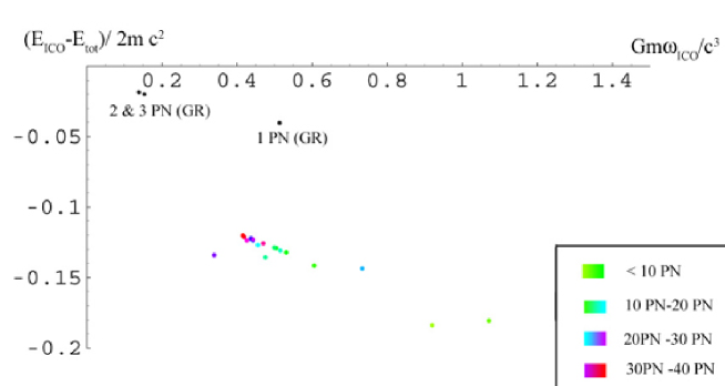
Figure 1: The PN ICO’s up to $38$ PN. ICO’s do not necessarily exist at each PN order. The series seem to converge whereas this can not be the case. ICO’s found in GR are also shown (extracted from BlanchetISCO3PN ).

5 Construction and convergence of a perturbative solution

Beyond the circular motion, which is not physical unless advanced and retarded waves are considered, we shall now construct an inspiral motion, solution of the only retarded EOM. When deriving a perturbative solution to the EOM, one find convenient to look for the orbital acceleration $\dot{\beta}$ as a function of $\beta$

$$\dot{\beta}(t)=f[\beta(t)],$$ (18)

which, together with the radius as a function of $\beta$, completely characterizes the motion. The perturbative expansion of the EOM goes as follow. We look for function $f$ and $r$ in power of a parameter $\varepsilon$, as $f=f_{0}+\varepsilon f_{1}+\ldots+\epsilon^{n}f_{n}+\ldots$ and similarly for $r$, where the $f_{i}$ and $r_{i}$ are unknown function of $\beta$, and $\varepsilon$ is an arbitrary parameter. We choose $f_{0}=0$ in order to recover an expansion whose 0-th order corresponds to the circular motion. It is important to note that this choice is analytically unmotivated, but rather corresponds to an initial condition assumption.

We have proven in NotreArticle that this expansion converges in powers of $\beta^{5}$, which means that the property $f_{i}\sim\mathcal{O}(1)$ and $r_{i}\sim\mathcal{O}(1)$ is satisfied when $\varepsilon=\beta^{5}$. Moreover, this amplitude is directly related to the first non-vanishing multipolar radiation of the binary, namely the quadrupolar one : $\dot{E}/E\sim\beta^{5}$, where $E$ is the energy of the binary. Note also that this expansion is not a PN one since each functions $f_{i}$ and $r_{i}$ are found to possess a complicated series expansion, and are not just monomials. For instance the 0-th order provides an analytical formula linking the radius of the circular motion to its orbital velocity, see Eq. (13). This method thus gives to each order many non-perturbative information.

6 Analytical and numerical results

We have run the previous algorithm up to the second order. It means that we have derived the exact, analytical expression of $f_{1}$, $f_{2}$, $r_{1}$ and $r_{2}$. We do not write explicitly these functions here since their expression are quite heavy, but a simple code enables to find them. These functions $f$ and $r$ fully characterize the motion, so that we will refer to these first and second order as the first and second order motion.

We can write the explicit and exact PN expansion of these two solutions. We show in NotreArticle that the first order of perturbation give both the acceleration and the radius exactly up to 4.5 PN, whereas the second order provides a correct radius up to $7$ PN. These results are :

$$\dot{\beta}_{\textrm{4.5 PN}}=\frac{c^{3}}{Gm}\left(\frac{512}{15}\beta^{9}-\frac{4864}{35}\beta^{11}+\frac{2316736}{2835}\beta^{13}-\frac{1216928}{297}\beta^{15}+\frac{5973800428}{289575}\beta^{17}+\mathcal{O}\left(\beta^{19}\right)\right)$$ (19)

$$r_{\textrm{7 PN}}=\frac{Gm}{c^{2}}\left(\frac{1}{4\beta^{2}}+\frac{1}{4}-\frac{5}{4}\beta^{2}+\frac{131}{36}\beta^{4}-\frac{617}{60}\beta^{6}-\frac{883}{84}\beta^{8}+\frac{111900409}{170100}\beta^{10}-\frac{119811886267}{13097700}\beta^{12}+\mathcal{O}\left(\beta^{13}\right)\right)$$ (20)

Let us now focus on the entire non perturbative functions. In the left panel of Fig. (2), we plot the orbital acceleration as a function of $\beta$. We show the behavior of this acceleration for the first and second order motion, and we also plot the 4.5 PN expansion of it given in Eq. (19). We also plot in the right panel of Fig. (2) the radius as a function of $\beta$, normalized to the Newtonian radius $r_{\textrm{Newton}}=Gm/4\beta^{2}c^{2}$. We show the circular radius, the first and second order one, and the 7PN radius given by Eq. (20).

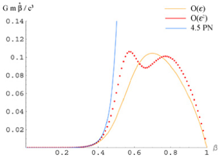
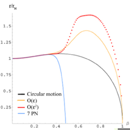
Figure 2: (left) The orbital acceleration as a function of $\beta$: the first order and second order solutions, compared to the $4.5$ PN one. (right) The radius of the orbit as a function of $\beta$. We plot the circular solution, and the first and second order corrections to it. The radius at $7$ PN is also given.

In NotreArticle , we also investigate the so-called Quasi-Equilibrium (QE) scheme which has been extensively used in GR (see, e.g, QEinGR ,QEinGR2 ) and discuss its validity in Nordström’s theory. This approximation holds if the dynamical (damping) timescale is much greater than the orbital period, so that the gravitational radiation can be neglected at first approximation, and the motion is quasi-circular. The left panel of Fig. (3) represents the ratio (at first order) of the orbital period over the dynamical damping timescale. We thus see that the QE approximation is an excellent one in the non-relativistic and in the ultra-relativistic regime. However, in the intermediate regime ($\beta\sim 0.6$) the dynamical timescale becomes comparable and even shorter than the orbital period, so that the orbit is highly non-circular and the approximation underlying the QE-scheme is strongly broken. This is the plunge phase of the binary.

A numerical integration of Eq. (18) yields the behavior of the norm of the velocity $\beta$ as a function of time, plotted in right panel of Fig. (3). The three curves corresponds to the 4.5 PN result, the first order and second order result, starting at $\beta=0.1$. The three results are very similar until $\beta\sim 0.4$. A major difference, however, between the PN solution and the non-perturbative solutions is that it cannot take into account the pole of special relativity, so that the PN solution diverges : $\beta(t)\to\infty$ in a finite time. The non-perturbative solutions, on the contrary, includes effects of special relativity, notably the fact that $\beta$ cannot be greater than $1$. It has the major effect to delay the moment of “coalescence” of the two body.

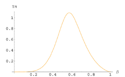
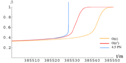
Figure 3: (left) The ratio of the delay-time over the dynamical damping timescale as a function of $\beta$ at first order. These two timescales become comparable in the relativistic regime.(right) The behavior of the velocity in time, using the first order solution, the second order one and the PN solution one.

Finally we plot the motion of one of the companion over a large range of $\beta$, and compare the results of the PN approximation, the first and second order approximations. This is shown in Fig. 4. Although the behavior of the PN solution is quite bad near $\beta=1$, we see that the three solutions agree very well until a separation of order $4m$ (a radius $2m$), which is not too much compared to the Schwarzschild radius. This might be seen as a good news for PN expansions.

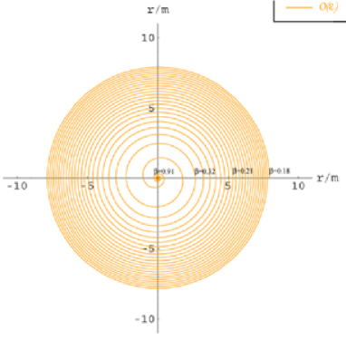
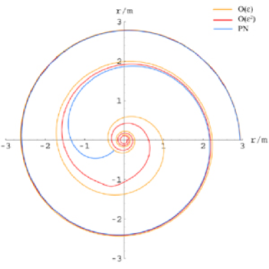
Figure 4: (left) The motion of one companion, from $\beta=.18$ to $\beta=.91$, using the first order result $f_{1}$. (right) The ultrarelativistic phase and the comparison of the first order solution (external line), the second order one (middle line) and the PN solution (interior line).

7 Conclusion and perspectives

The aim of this work was to extract as much as possible analytical results concerning the two-body problem in Nordström’s theory, which is without doubts the purely scalar theory of gravity closest to GR. Once again, these analytical results are not a priori of direct interest as far as the construction of relevant templates is concerned, but are interesting since they enable to estimate the validity of methods used in the two-body problem in GR. For instance, analytical results derived here should be useful to test the efficiency of numerical codes. Those analytical results are already summarized in the introduction.

Of course, an exact solution of the equation of motion may be one day derived, and that will be of great interest. Further work on the validity of the QE-scheme may also be done, see NotreArticle . It could also be interesting to examine the behavior of the PN expansion in the plunge phase, compared to a numerical solution of the full equation of motion. We could therefore check if the PN predictions are very bad ones in the ultra relativistic limit (as expected, since the small parameter goes to $1$), or if, due to some non-trivial cancellations (note for example the alternate signs in Eq. (19) and Eq. (20)), the PN picture reveals itself to be a good one. Such an alternation has already been observed in PN expansion of GR, see Alternancesignes . This behavior has not been explained yet, and we suggest that it might be understood in Nortsröm’s theory.

References

- (1) S. Nissanke, L. Blanchet, Class. Quantum Grav. 22, 1007-1032 (2005).
- (2) S. L. Shapiro, S. A. Teukolsky, Phys. Rev. D47, 1529-1540 (1993).
- (3) K. Watt and C. W. Misner, Relativistic scalar gravity : a laboratory for numerical relativity, gr-qc/9910032.
- (4) H-J. Yo, T. W. Baumgarte, S. L. Shapiro, Phys. Rev. D63, 064035 (2001).
- (5) J. P. Bruneton, G. Esposito-Farèse, The two-body problem in Nordström’s scalar theory of gravity, to be published.
- (6) C. W. Misner, K. S. Thorne and J. A. Wheeler, Gravitation (Freeman, San Francisco, 1973).
- (7) T. Damour and G. Esposito-Farèse, Class. Quantum Grav. 9, 2093 (1992).
- (8) A. Einstein and A. D. Fokker, Ann. d. Phys. 44, 321 (1914).
- (9) T. Damour, Les Houches 1992, Proceedings, Gravitation and quantizations, 1-61.
- (10) G. Nordström, Ann. d. Phys. 42, 533, (1913).
- (11) G. Nordström, Phys. Zeit. 13, 1126, (1912).
- (12) F. Ravndal, Scalar gravitation and extra dimensions, gr-qc/0405030.
- (13) E. Poisson, An introduction to the Lorentz-Dirac equation, gr-qc/9912045.
- (14) P. A. M. Dirac, Proc. Roy. Soc. London A167, 148 (1938).
- (15) T. Damour Classical renormalizations PHD thesis, unpublished
- (16) L. Blanchet, Phys. Rev. D65, 124009 (2002).
- (17) T. W. Baumgarte, The innermost stable circular orbit in compact binaries, Philadelphia (2000), Astrophysical sources for ground-based gravitational wave detectors, 176-188 (also gr-qc/0101045).
- (18) J. L. Friedman and K. Ury, Post-Minkowski action for point-particles and a Helically symmetric binary solution, gr-qc/0510002
- (19) T. W. Baumgarte, G. B. Cook, M. A. Scheel, S. L. Shapiro, S. A. Teukolsky, Phys. Rev. D57, 7299 (1998).
- (20) S. Bonazzola, E. Gourgoulhon, J.-A. Marck, Phys. Rev. Lett. 82, 892-895 (1999) ; E. Gourgoulhon, P. Grandclément, K. Taniguchi, J.-A. Marck, S. Bonazzola, Phys. Rev. D63, 064029, (2001).
- (21) L. Blanchet, G. Faye, B. R. Iyer, B. Joguet, Phys. Rev. D65, 061501 (2002).